Download as PDF, PPTX
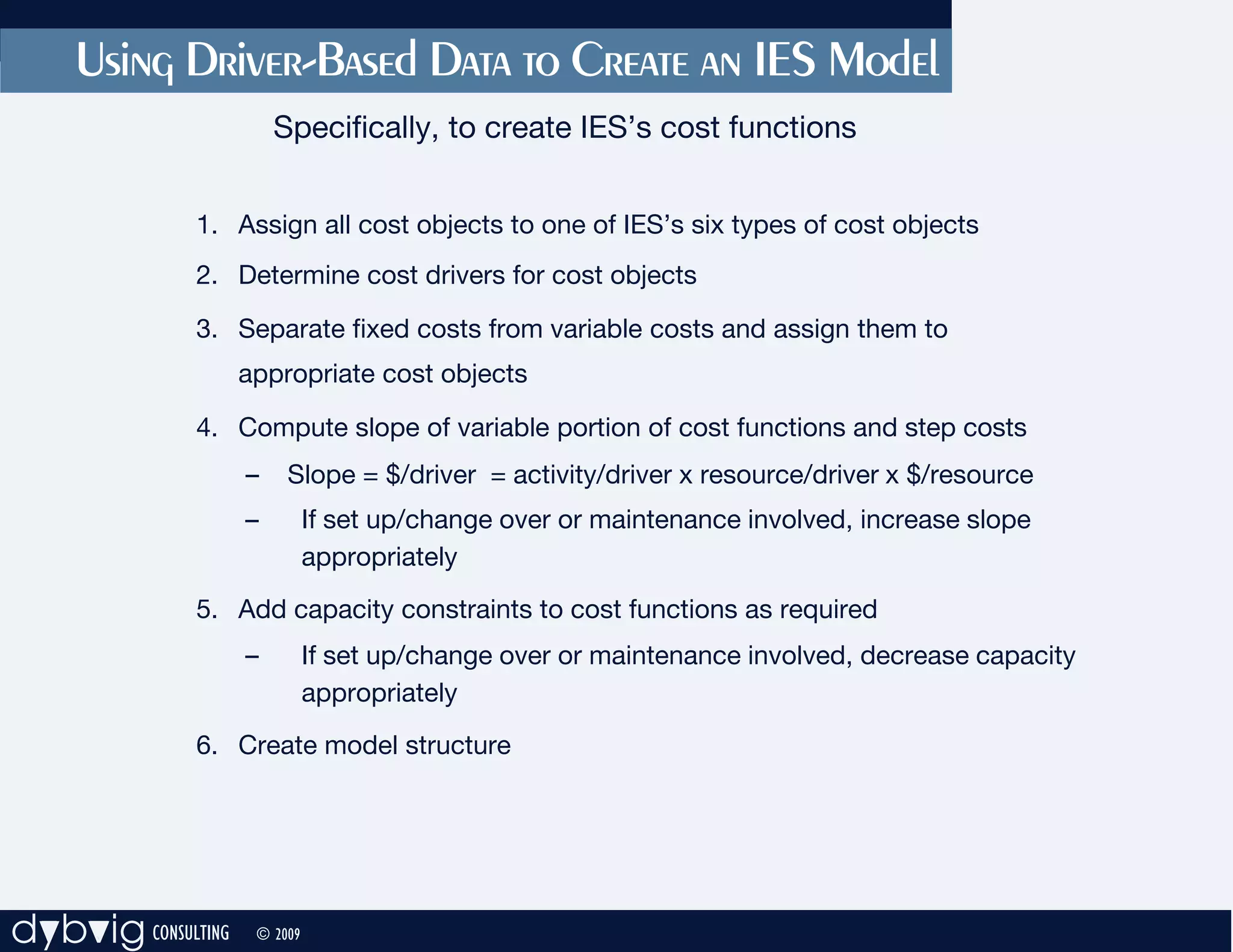
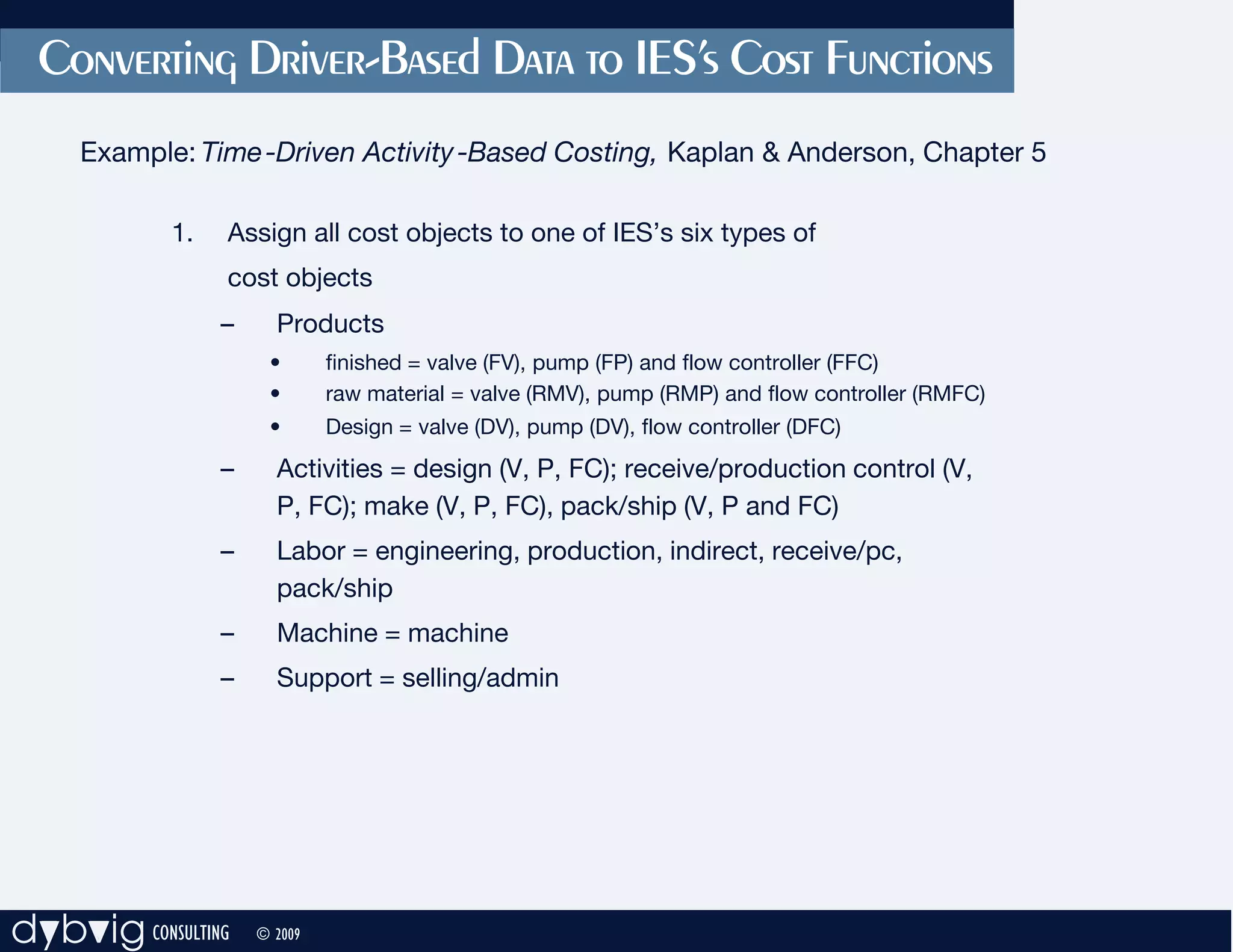
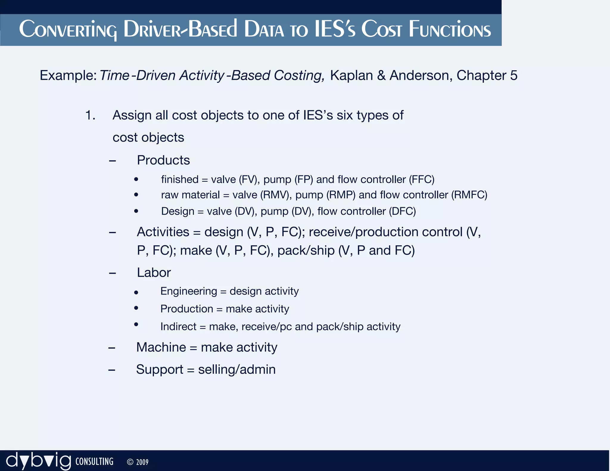
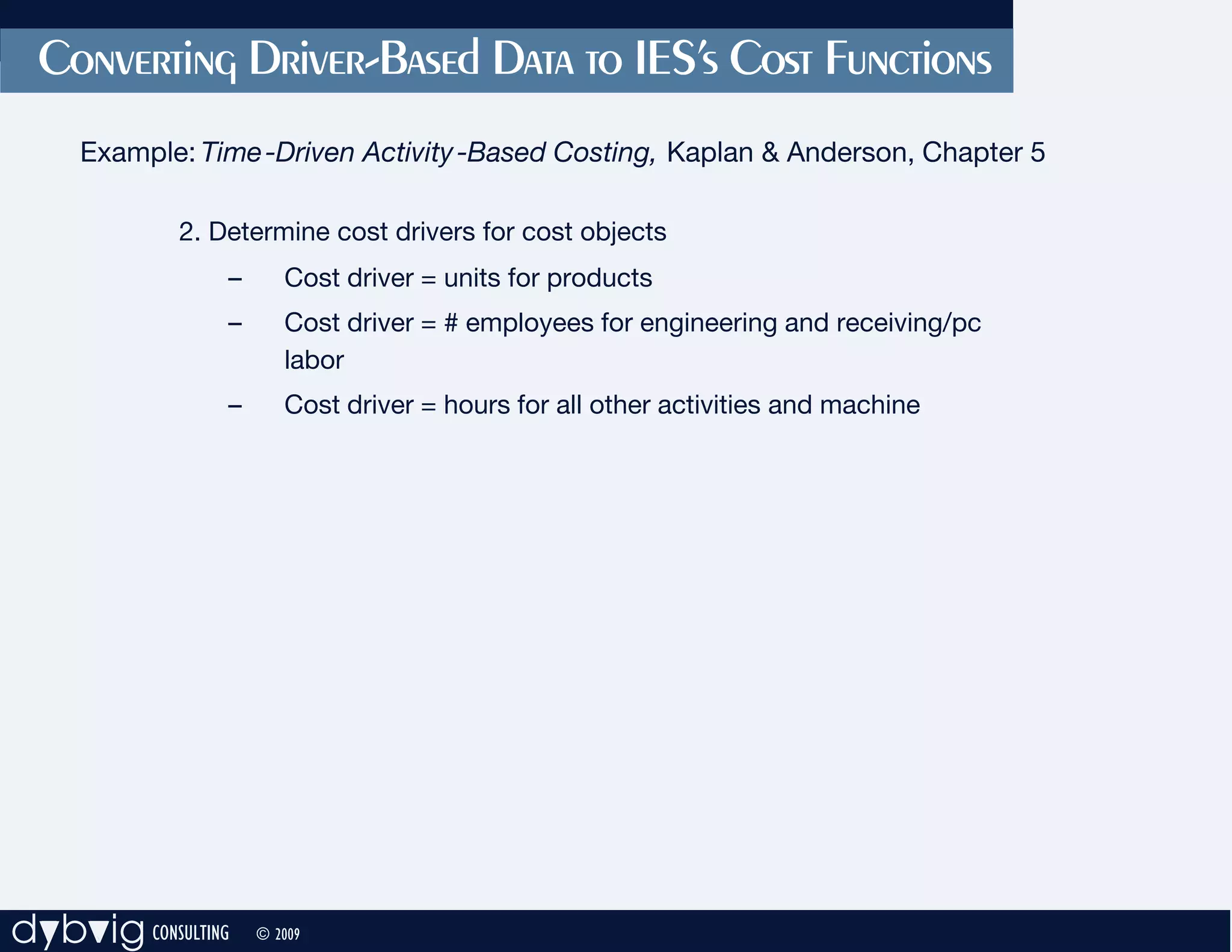
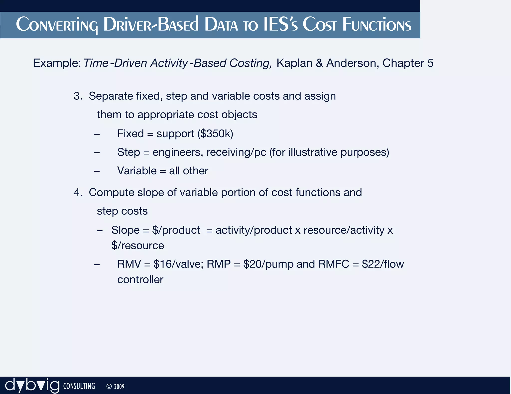

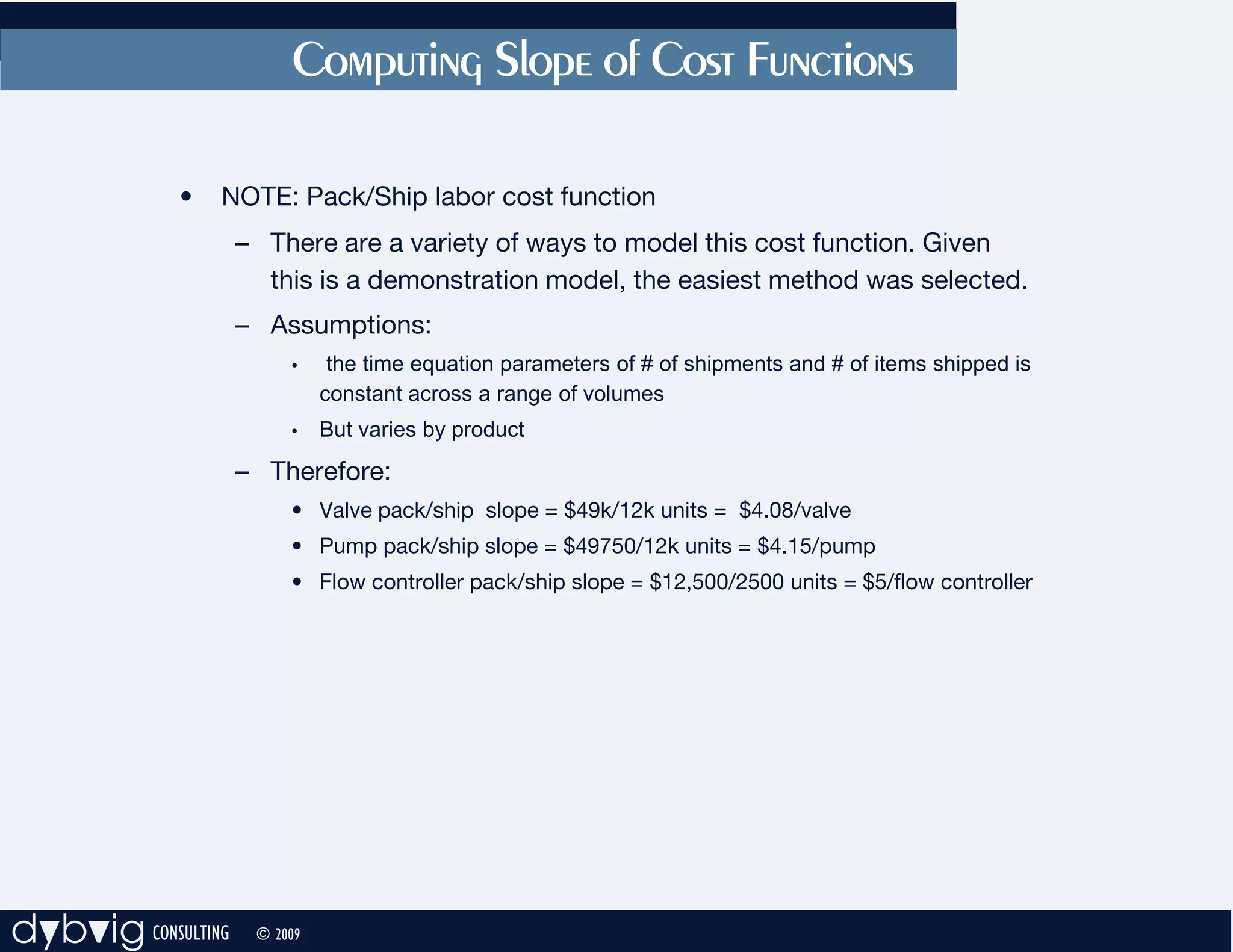
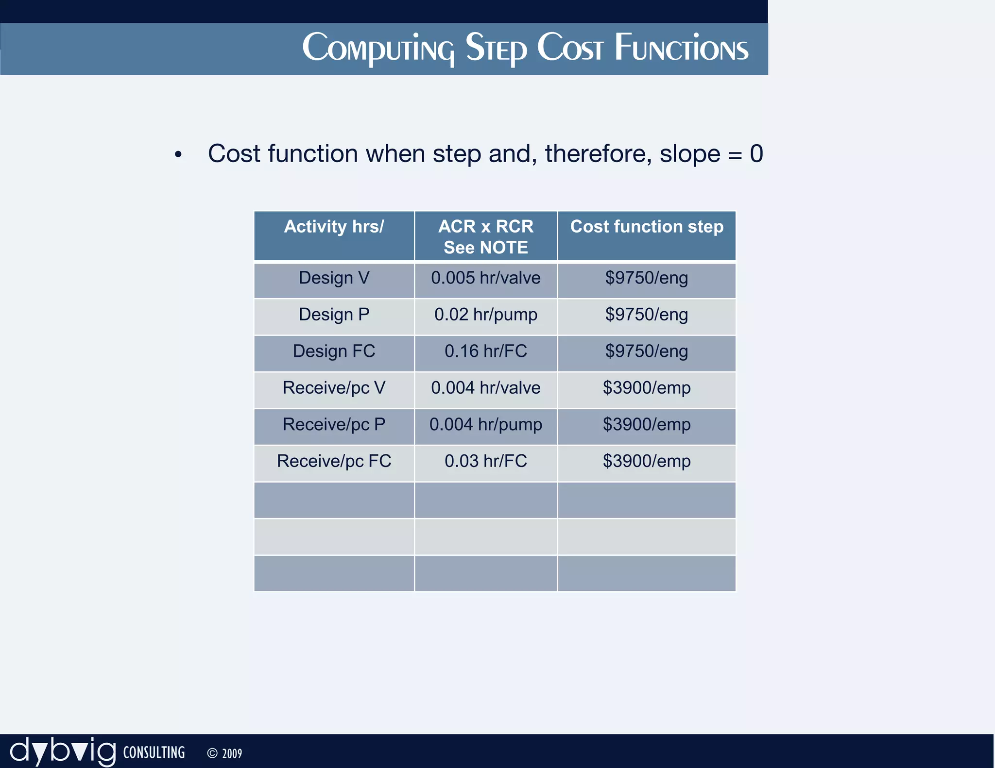

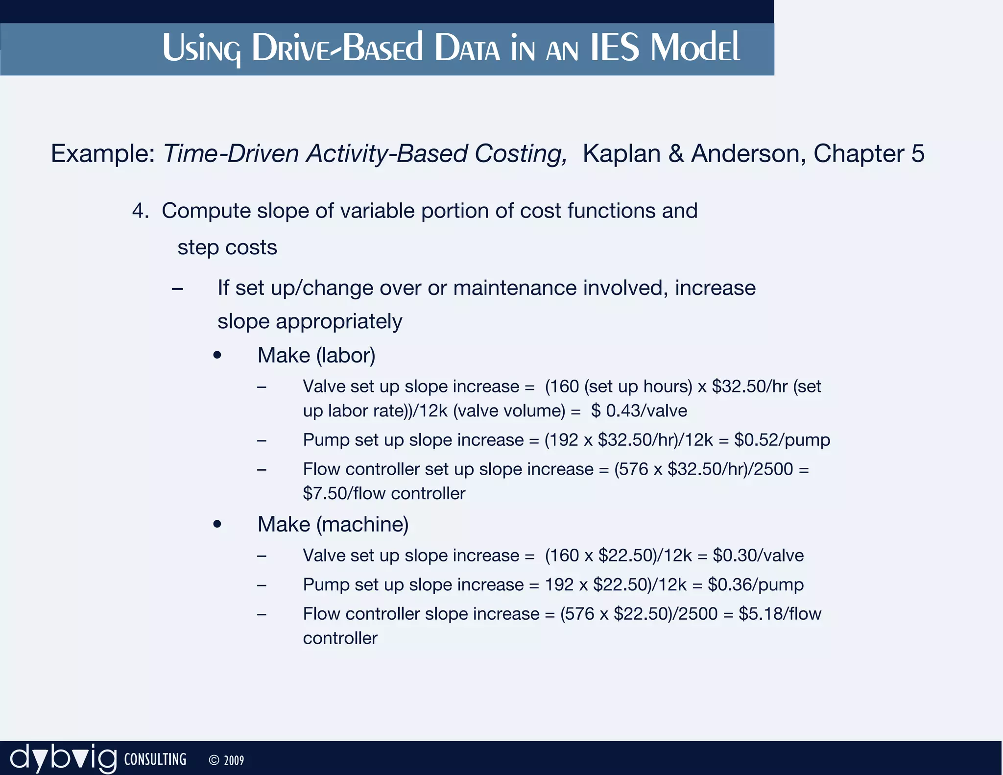
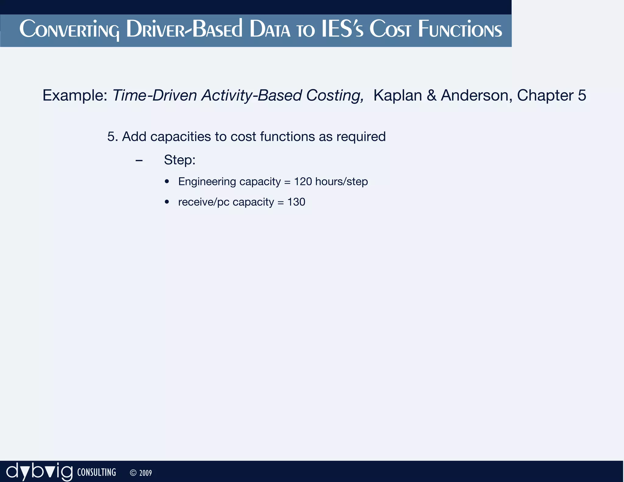
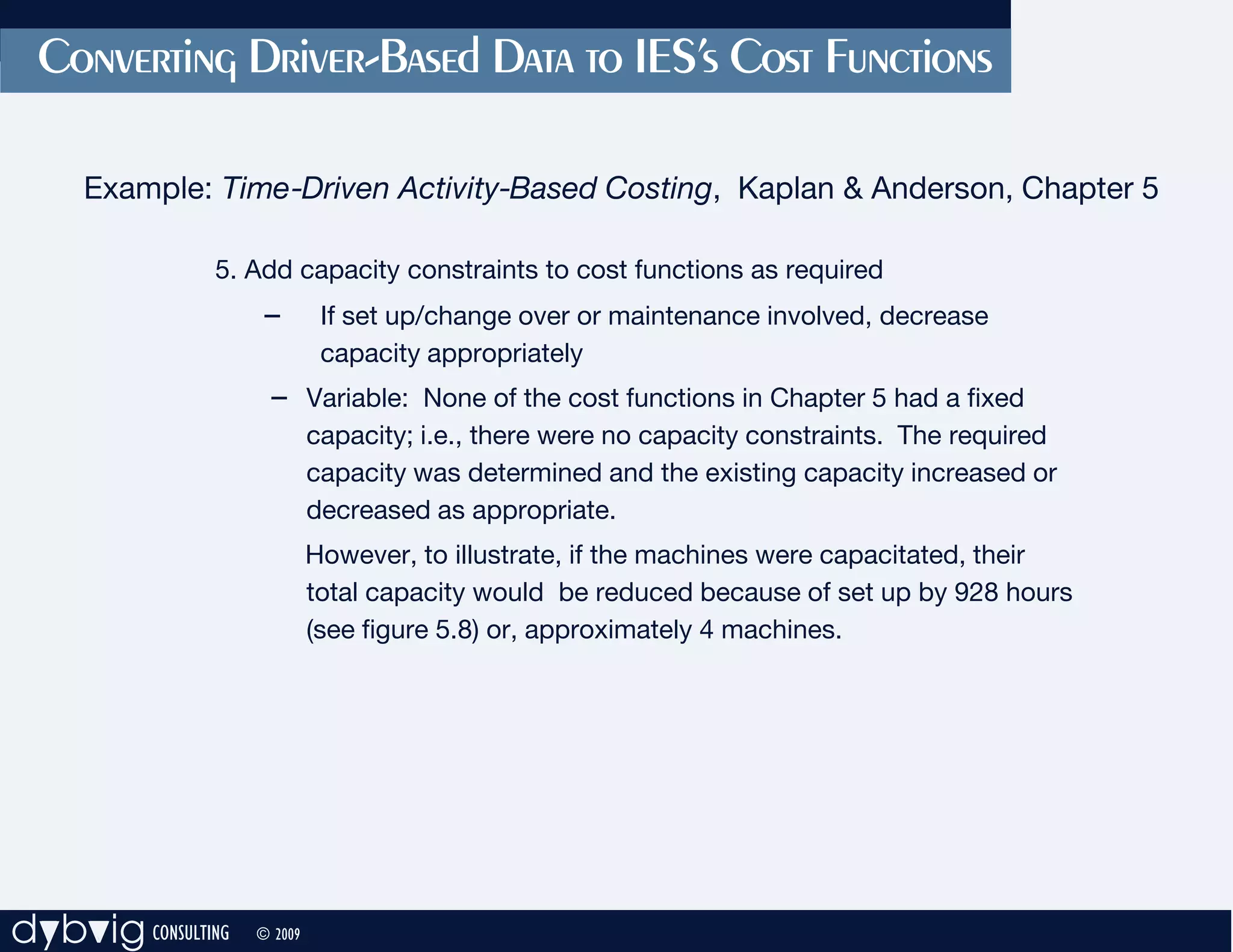

1. The document describes how to create cost functions in IES using driver-based data by assigning cost objects to categories, determining cost drivers, separating fixed and variable costs, computing slopes of variable cost functions and step costs, and adding capacity constraints. 2. It provides an example using time-driven activity-based costing data from a company that produces valves, pumps, and flow controllers. Cost objects are assigned to product, activity, labor, machine, and support categories. 3. Cost drivers, fixed costs, variable costs, slopes, and step costs are computed for various cost objects like raw materials, design, receiving, packing, and shipping based on activity rates, resource costs, and product volumes.


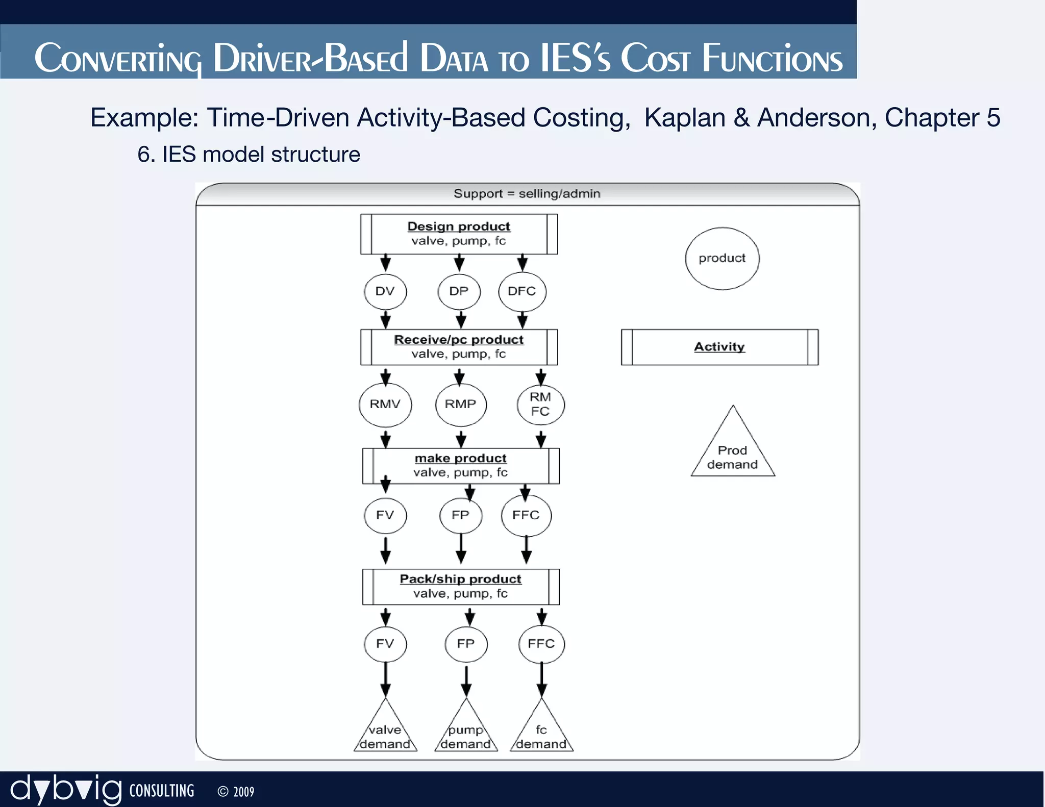
![Vibe Coding vs. Spec-Driven Development [Free Meetup]](https://cdn.slidesharecdn.com/ss_thumbnails/vibecodingvsspecdrivendevelopment-251209105622-43f455e7-thumbnail.jpg?width=640&height=640&fit=bounds)


