Downloaded 69 times


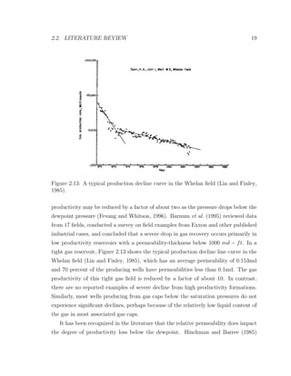

![60 CHAPTER 3. EXPERIMENTAL INVESTIGATION
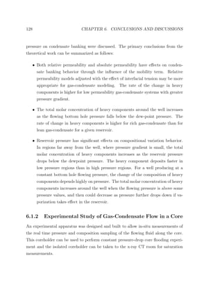
where the subscripts l and a represent liquid-phase and air-phase CT numbers,
whereas lr and ar refer to liquid- and air-saturation rock respectively. Thus, the
saturation of gas in each voxel is defined as:
Sg =
CTlr − CTgr
CTlr − CTglr
(3.10)
Thus to calculate the two-phase saturation, we need to have three parameters:
CTlr, CTgr, and CTglr. Due to the difficulty of discharging the hydrocarbon exhaust
in the CT room, the three parameters were measured separately. The core saturated
with liquid butane at 40 psi and gaseous methane at atmosphere pressure was first
scanned and after the flow test experiment, the isolated core filled with mixture
at high pressure was then taken to the CT room to measure CTglr. Fluid density,
especially gas density, normally changes with pressure, and according to Vinegar and
Wellington (1987), the linear attenuation coefficient is expressed as:
µ = [σ(E) + b ¯Z3.8
/E3.2
]ρ (3.11)
where σ(E) is the Klein-Nishina Coefficient, ρ is the electron density, ¯Z is the effective
atomic number, E is the photon energy in keV , and b is a constant. Eq. 3.11 shows
that fluids with greater density have greater linear attenuation coefficient. The CTlr
and CTgr were measured at relatively very low pressure (40 psi for the core saturated
with liquid butane, and atmosphere pressure for the core saturated with gaseous
methane), hence pressure adjustment for fluid density is needed to ensure that CTlr
and CTgr are measured/calculated at the same pressure as the high mixture pressure.
Due to the relatively small compressibility, we can assume that the sandstone matrix
density and the pore volume does not change with pressure, thus the change in the
µr is mainly due to the change of fluid in the pore space.
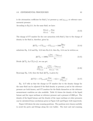
∆µfr = µfr(p) − µfr(ref) = φ[µf(p) − µf(ref)] (3.12)
where µfr is the attenuation coefficient for the core saturated with fluid f, and µf(p)](https://image.slidesharecdn.com/gascondensationprocess-150223031138-conversion-gate02/85/Gas-condensation-process-82-320.jpg)


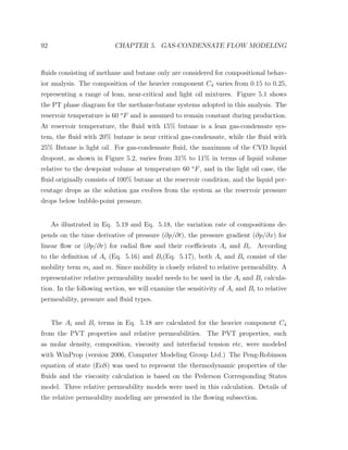
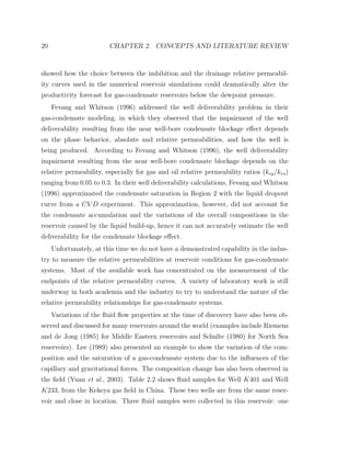
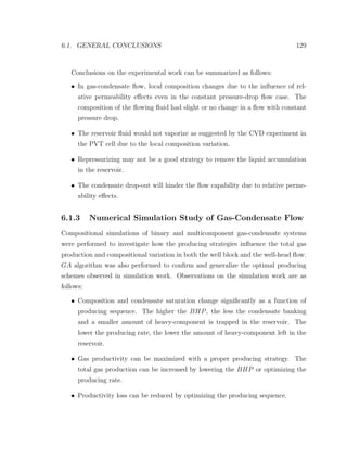
![5.2. COMPOSITIONAL VARIATION BEHAVIOR 95
where σ is the IFT, σ∗
is a reference IFT, krcm and krgm are the condensate and
gas relative permeabilities at complete miscibility, the immiscible krci and krgi are the
condensate and gas relative permeabilities for the fluids at IFT values equal to or
greater than σ∗
, and n is an adjustable exponent. Eq. 5.20 and Eq. 5.21 states that
the relative permeability transition function is a mixing model as a function of IFT.
Based on experimental data, Hartman and Cullick (1994) suggested a correlation
for residual condensate saturation to gas as a function of IFT:
Scrg(σ) = [1 + 0.67log(
σ
σ∗
)]Scrgi (5.23)
The gas endpoint is:
Sgc(σ) =
σ
σ∗
Sgc (5.24)
The miscible relative permeability used in the mixing function is normalized with
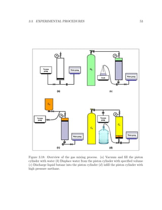
respect to the IFT dependent endpoints:
krcm =
1 − Scrg(σ) − Sg
1 − Scrg(σ)
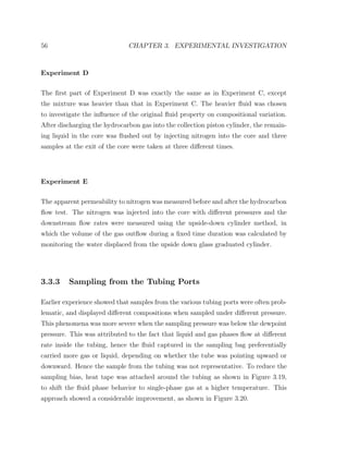
(5.25)
krgm =
Sg
1 − Sgc(σ)
(5.26)
When the fluid condition is far away from the critical point, the phase interface is
distinct. The permeabilities of the liquid and vapor phase can be approximated with
Eq. 5.27 and Eq. 5.28:
krci = [
1 − Scrg(σ) − Sg
1 − Scrg(σ)
]2
(5.27)
krgi = [
Sg
1 − Sgc(σ)
]2
(5.28)
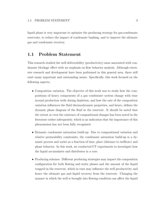
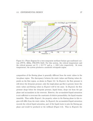
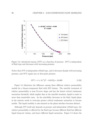
Figure 5.3 shows the calculated interfacial tension (IFT) correlated with pressure
data for the three binary fluids used in this compositional analysis. A good rela-
tionship (Eq. 5.29) between IFT and pressure can be inferred from the correlation.](https://image.slidesharecdn.com/gascondensationprocess-150223031138-conversion-gate02/85/Gas-condensation-process-117-320.jpg)
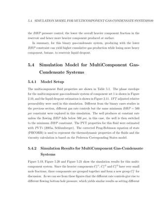
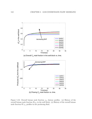
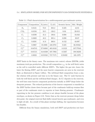
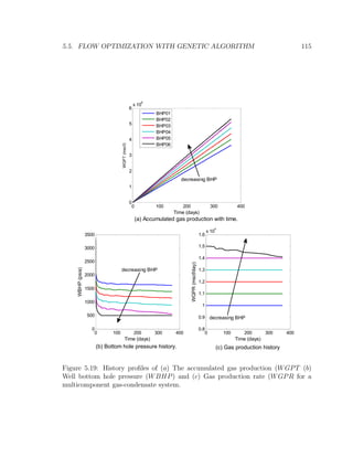
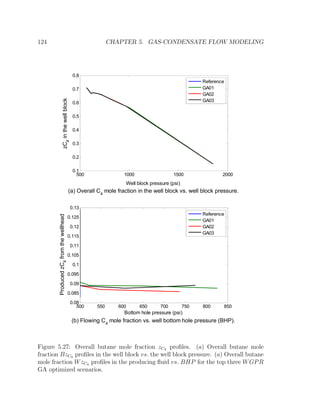
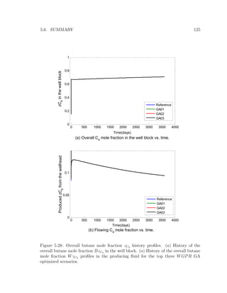


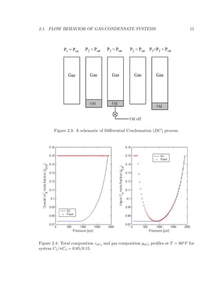
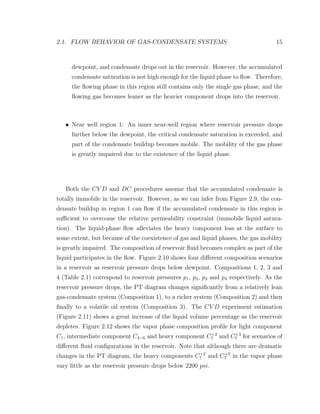
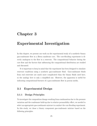
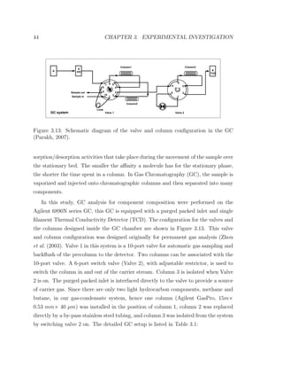
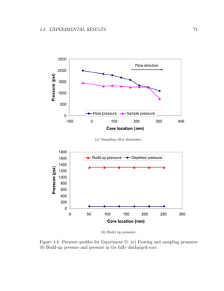
This document is a dissertation submitted by Chunmei Shi to Stanford University in partial fulfillment of the requirements for a Doctor of Philosophy degree. The dissertation investigates the flow behavior of gas-condensate wells through experimental and numerical modeling. Chapter 1 introduces the problem of productivity losses in gas-condensate reservoirs due to liquid dropout near the wellbore. Chapters 2-5 describe experimental investigations of gas-condensate flow through a core and numerical simulations to model compositional variations. Chapter 5 also uses optimization techniques to improve recovery. The conclusions indicate the work developed theoretical models, experimentally studied flow in a core, and numerically simulated gas-condensate flow to increase productivity from gas-condensate reservoirs.


