Stochastic Differential Equations For Science And Engineering Uffe Hgsbro Thygesen
Stochastic Differential Equations For Science And Engineering Uffe Hgsbro Thygesen
Stochastic Differential Equations For Science And Engineering Uffe Hgsbro Thygesen
Stochastic Differential Equations For Science And Engineering Uffe Hgsbro Thygesen
Stochastic Differential Equations For Science And Engineering Uffe Hgsbro Thygesen
1.
Stochastic Differential EquationsFor Science
And Engineering Uffe Hgsbro Thygesen download
https://ebookbell.com/product/stochastic-differential-equations-
for-science-and-engineering-uffe-hgsbro-thygesen-49482446
Explore and download more ebooks at ebookbell.com
2.
Here are somerecommended products that we believe you will be
interested in. You can click the link to download.
Stochastic Differential Equations For Science And Engineering Uffe
Hgsbro Thygesen
https://ebookbell.com/product/stochastic-differential-equations-for-
science-and-engineering-uffe-hgsbro-thygesen-48640724
Stochastic Partial Differential Equations For Computer Vision With
Uncertain Data Tobias Preusser
https://ebookbell.com/product/stochastic-partial-differential-
equations-for-computer-vision-with-uncertain-data-tobias-
preusser-46201506
Amplitude Equations For Stochastic Partial Differential Equations Dirk
Blomker
https://ebookbell.com/product/amplitude-equations-for-stochastic-
partial-differential-equations-dirk-blomker-4646848
Stochastic Calculus And Differential Equations For Physics And Finance
1st Edition Mccauley
https://ebookbell.com/product/stochastic-calculus-and-differential-
equations-for-physics-and-finance-1st-edition-mccauley-55493330
3.
Stochastic Calculus AndDifferential Equations For Physics And Finance
2013th Edition Joseph L Mccauley
https://ebookbell.com/product/stochastic-calculus-and-differential-
equations-for-physics-and-finance-2013th-edition-joseph-l-
mccauley-87466206
Simulation And Inference For Stochastic Differential Equations With R
Examples 1st Edition Stefano M Iacus Auth
https://ebookbell.com/product/simulation-and-inference-for-stochastic-
differential-equations-with-r-examples-1st-edition-stefano-m-iacus-
auth-1143124
Statistical Methods For Stochastic Differential Equations Mathieu
Kessler
https://ebookbell.com/product/statistical-methods-for-stochastic-
differential-equations-mathieu-kessler-2633472
Asymptotic Analysis For Functional Stochastic Differential Equations
1st Edition Jianhai Bao
https://ebookbell.com/product/asymptotic-analysis-for-functional-
stochastic-differential-equations-1st-edition-jianhai-bao-5696484
Path Regularity For Stochastic Differential Equations In Banach Spaces
Johanna Dettweiler
https://ebookbell.com/product/path-regularity-for-stochastic-
differential-equations-in-banach-spaces-johanna-dettweiler-988944
6.
Stochastic Differential
Equations forScience and
Engineering
Stochastic Differential Equations for Science and Engineering is aimed at
students at the M.Sc. and PhD level. The book describes the mathematical con-
struction of stochastic differential equations with a level of detail suitable to the
audience, while also discussing applications to estimation, stability analysis, and
control. The book includes numerous examples and challenging exercises. Com-
putational aspects are central to the approach taken in the book, so the text is
accompanied by a repository on GitHub containing a toolbox in R which imple-
ments algorithms described in the book, code that regenerates all figures, and
solutions to exercises.
Features
• Contains numerous exercises, examples, and applications
• Suitable for science and engineering students at Master’s or PhD level
• Thorough treatment of the mathematical theory combined with an accessible
treatment of motivating examples
• GitHub repository available at: https://github.com/Uffe-H-Thygesen/SDE-
book and https://github.com/Uffe-H-Thygesen/SDEtools
Uffe Høgsbro Thygesen received his Ph.D. degree from the Technical University
of Denmark in 1999, based on a thesis on stochastic control theory. He worked
with applications to marine ecology and fisheries until 2017, where he joined the
Department of Applied Mathematics and Computer Science at the same univer-
sity. His research interests are centered on deterministic and stochastic dynamic
systems and involve times series analysis, control, and dynamic games, primarily
with applications in life science. In his spare time he teaches sailing and kayaking
and learns guitar and photography.
Contents
Preface xiii
Chapter 1 Introduction 1
Section I Fundamentals
Chapter 2 Diffusive Transport and Random Walks 11
2.1 DIFFUSIVE TRANSPORT 12
2.1.1 The Conservation Equation 13
2.1.2 Fick’s Laws 14
2.1.3 Diffusive Spread of a Point Source 15
2.1.4 Diffusive Attenuation of Waves 17
2.2 ADVECTIVE AND DIFFUSIVE TRANSPORT 19
2.3 DIFFUSION IN MORE THAN ONE DIMENSION 20
2.4 RELATIVE IMPORTANCE OF ADVECTION AND DIFFU-
SION 22
2.5 THE MOTION OF A SINGLE MOLECULE 23
2.6 MONTE CARLO SIMULATION OF PARTICLE MOTION 27
2.7 CONCLUSION 28
2.8 EXERCISES 29
Chapter 3 Stochastic Experiments and Probability Spaces 31
3.1 STOCHASTIC EXPERIMENTS 32
3.2 RANDOM VARIABLES 36
3.3 EXPECTATION IS INTEGRATION 38
3.4 INFORMATION IS A σ-ALGEBRA 40
v
11.
vi Contents
3.5CONDITIONAL EXPECTATIONS 42
3.5.1 Properties of the Conditional Expectation 44
3.5.2 Conditional Distributions and Variances 45
3.6 INDEPENDENCE AND CONDITIONAL INDEPENDENCE 47
3.7 LINEAR SPACES OF RANDOM VARIABLES 49
3.8 CONCLUSION 52
3.9 NOTES AND REFERENCES 53
3.9.1 The Risk-Free Measure 54
3.9.2 Convergence for Sequences of Events 54
3.9.3 Convergence for Random Variables 56
3.10 EXERCISES 60
Chapter 4 Brownian Motion 63
4.1 STOCHASTIC PROCESSES AND RANDOM FUNC-
TIONS 64
4.2 DEFINITION OF BROWNIAN MOTION 64
4.3 PROPERTIES OF BROWNIAN MOTION 66
4.4 FILTRATIONS AND ACCUMULATION OF INFORMATION 77
4.5 THE MARTINGALE PROPERTY 77
4.6 CONCLUSION 83
4.7 NOTES AND REFERENCES 83
4.8 EXERCISES 84
Chapter 5 Linear Dynamic Systems 89
5.1 LINEAR SYSTEMS WITH DETERMINISTIC INPUTS 90
5.2 LINEAR SYSTEMS IN THE FREQUENCY DOMAIN 91
5.3 A LINEAR SYSTEM DRIVEN BY NOISE 94
5.4 STATIONARY PROCESSES IN TIME DOMAIN 94
5.5 STATIONARY PROCESSES IN FREQUENCY DOMAIN 97
5.6 THE RESPONSE TO NOISE 99
5.7 THE WHITE NOISE LIMIT 101
5.8 INTEGRATED WHITE NOISE IS BROWNIAN MOTION 103
5.9 LINEAR SYSTEMS DRIVEN BY WHITE NOISE 105
5.10 THE ORNSTEIN-UHLENBECK PROCESS 107
12.
Contents vii
5.11THE NOISY HARMONIC OSCILLATOR 108
5.12 CONCLUSION 109
5.13 EXERCISES 111
Section II Stochastic Calculus
Chapter 6 Stochastic Integrals 117
6.1 ORDINARY DIFFERENTIAL EQUATIONS DRIVEN BY
NOISE 117
6.2 SOME EXEMPLARY EQUATIONS 120
6.2.1 Brownian Motion with Drift 120
6.2.2 The Double Well 120
6.2.3 Geometric Brownian Motion 121
6.2.4 The Stochastic van der Pol Oscillator 122
6.3 THE ITÔ INTEGRAL AND ITS PROPERTIES 123
6.4 A CAUTIONARY EXAMPLE:
T
0 BS dBS 126
6.5 ITÔ PROCESSES AND SOLUTIONS TO SDES 129
6.6 RELAXING THE L2 CONSTRAINT 131
6.7 INTEGRATION WITH RESPECT TO ITÔ PROCESSES 132
6.8 THE STRATONOVICH INTEGRAL 133
6.9 CALCULUS OF CROSS-VARIATIONS 135
6.10 CONCLUSION 136
6.11 NOTES AND REFERENCES 137
6.11.1 The Proof of Itô Integrability 137
6.11.2 Weak Solutions to SDE’s 138
6.12 EXERCISES 138
Chapter 7 The Stochastic Chain Rule 141
7.1 THE CHAIN RULE OF DETERMINISTIC CALCULUS 142
7.2 TRANSFORMATIONS OF RANDOM VARIABLES 142
7.3 ITÔ’S LEMMA: THE STOCHASTIC CHAIN RULE 143
7.4 SOME SDE’S WITH ANALYTICAL SOLUTIONS 146
7.4.1 The Ornstein-Uhlenbeck Process 148
7.5 DYNAMICS OF DERIVED QUANTITIES 150
7.5.1 The Energy in a Position-Velocity System 150
13.
viii Contents
7.5.2The Cox-Ingersoll-Ross Process and the Bessel
Processes 151
7.6 COORDINATE TRANSFORMATIONS 152
7.6.1 Brownian Motion on the Circle 153
7.6.2 The Lamperti Transform 153
7.6.3 The Scale Function 154
7.7 TIME CHANGE 156
7.8 STRATONOVICH CALCULUS 159
7.9 CONCLUSION 162
7.10 NOTES AND REFERENCES 163
7.11 EXERCISES 163
Chapter 8 Existence, Uniqueness, and Numerics 167
8.1 THE INITIAL VALUE PROBLEM 168
8.2 UNIQUENESS OF SOLUTIONS 168
8.2.1 Non-Uniqueness: The Falling Ball 168
8.2.2 Local Lipschitz Continuity Implies Uniqueness 169
8.3 EXISTENCE OF SOLUTIONS 172
8.3.1 Linear Bounds Rule Out Explosions 173
8.4 NUMERICAL SIMULATION OF SAMPLE PATHS 175
8.4.1 The Strong Order of the Euler-Maruyama Method
for Geometric Brownian Motion 176
8.4.2 Errors in the Euler-Maruyama Scheme 177
8.4.3 The Mil’shtein Scheme 178
8.4.4 The Stochastic Heun Method 180
8.4.5 The Weak Order 181
8.4.6 A Bias/Variance Trade-off in Monte Carlo Methods 183
8.4.7 Stability and Implicit Schemes 184
8.5 CONCLUSION 186
8.6 NOTES AND REFERENCES 187
8.6.1 Commutative Noise 188
8.7 EXERCISES 189
Chapter 9 The Kolmogorov Equations 191
9.1 BROWNIAN MOTION IS A MARKOV PROCESS 192
14.
Contents ix
9.2DIFFUSIONS ARE MARKOV PROCESSES 193
9.3 TRANSITION PROBABILITIES AND DENSITIES 194
9.3.1 The Narrow-Sense Linear System 197
9.4 THE BACKWARD KOLMOGOROV EQUATION 198
9.5 THE FORWARD KOLMOGOROV EQUATION 201
9.6 DIFFERENT FORMS OF THE KOLMOGOROV EQUA-
TIONS 203
9.7 DRIFT, NOISE INTENSITY, ADVECTION, AND DIFFU-
SION 204
9.8 STATIONARY DISTRIBUTIONS 206
9.9 DETAILED BALANCE AND REVERSIBILITY 209
9.10 CONCLUSION 212
9.11 NOTES AND REFERENCES 213
9.11.1 Do the Transition Probabilities Admit Densities? 213
9.11.2 Eigenfunctions, Mixing, and Ergodicity 215
9.11.3 Reflecting Boundaries 217
9.11.4 Girsanov’s Theorem 219
9.11.5 Numerical Computation of Transition Probabilities 220
9.11.5.1 Solution of the Discretized Equations 223
9.12 EXERCISES 224
Section III Applications
Chapter 10 State Estimation 233
10.1 RECURSIVE FILTERING 234
10.2 OBSERVATION MODELS AND THE STATE LIKELIHOOD 235
10.3 THE RECURSIONS: TIME UPDATE AND DATA UPDATE 238
10.4 THE SMOOTHING FILTER 241
10.5 SAMPLING TYPICAL TRACKS 243
10.6 LIKELIHOOD INFERENCE 244
10.7 THE KALMAN FILTER 246
10.7.1 Fast Sampling and Continuous-Time Filtering 249
10.7.2 The Stationary Filter 251
10.7.3 Sampling Typical Tracks 252
10.8 ESTIMATING STATES AND PARAMETERS AS A MIXED-
EFFECTS MODEL 253
15.
x Contents
10.9CONCLUSION 256
10.10 NOTES AND REFERENCES 257
10.11 EXERCISES 258
Chapter 11 Expectations to the Future 261
11.1 DYNKIN’S FORMULA 262
11.2 EXPECTED EXIT TIMES FROM BOUNDED DOMAINS 263
11.2.1 Exit Time of Brownian Motion with Drift on the
Line 263
11.2.2 Exit Time from a Sphere, and the Diffusive Time
Scale 265
11.2.3 Exit Times in the Ornstein-Uhlenbeck Process 265
11.2.4 Regular Diffusions Exit Bounded Domains in Fi-
nite Time 267
11.3 ABSORBING BOUNDARIES 269
11.4 THE EXPECTED POINT OF EXIT 271
11.4.1 Does a Scalar Diffusion Exit Right or Left? 272
11.5 RECURRENCE OF BROWNIAN MOTION 273
11.6 THE POISSON EQUATION 275
11.7 ANALYSIS OF A SINGULAR BOUNDARY POINT 276
11.8 DISCOUNTING AND THE FEYNMAN-KAC FORMULA 279
11.8.1 Pricing of Bonds 281
11.8.2 Darwinian Fitness and Killing 282
11.8.3 Cumulated Rewards 284
11.8.4 Vertical Motion of Zooplankton 285
11.9 CONCLUSION 286
11.10 NOTES AND REFERENCES 288
11.11 EXERCISES 288
Chapter 12 Stochastic Stability Theory 291
12.1 THE STABILITY PROBLEM 292
12.2 THE SENSITIVITY EQUATIONS 293
12.3 STOCHASTIC LYAPUNOV EXPONENTS 295
12.3.1 Lyapunov Exponent for a Particle in a Potential 298
12.4 EXTREMA OF THE STATIONARY DISTRIBUTION 299
16.
Contents xi
12.5A WORKED EXAMPLE: A STOCHASTIC PREDATOR-
PREY MODEL 301
12.6 GEOMETRIC BROWNIAN MOTION REVISITED 306
12.7 STOCHASTIC LYAPUNOV FUNCTIONS 308
12.8 STABILITY IN MEAN SQUARE 311
12.9 STOCHASTIC BOUNDEDNESS 313
12.10 CONCLUSION 316
12.11 NOTES AND REFERENCES 317
12.12 EXERCISES 317
Chapter 13 Dynamic Optimization 321
13.1 MARKOV DECISION PROBLEMS 322
13.2 CONTROLLED DIFFUSIONS AND PERFORMANCE
OBJECTIVES 325
13.3 VERIFICATION AND THE HAMILTON-JACOBI-BELLMAN
EQUATION 326
13.4 PORTFOLIO SELECTION 328
13.5 MULTIVARIATE LINEAR-QUADRATIC CONTROL 329
13.6 STEADY-STATE CONTROL PROBLEMS 331
13.6.1 Stationary LQR Control 333
13.7 DESIGNING AN AUTOPILOT 335
13.8 DESIGNING A FISHERIES MANAGEMENT SYSTEM 337
13.9 A FISHERIES MANAGEMENT PROBLEM IN 2D 339
13.10 OPTIMAL DIEL VERTICAL MIGRATIONS 341
13.11 CONCLUSION 343
13.12 NOTES AND REFERENCES 345
13.12.1 Control as PDE-Constrained Optimization 346
13.12.2 Numerical Analysis of the HJB Equation 346
13.13 EXERCISES 351
Chapter 14 Perspectives 353
Bibliography 355
Index 361
18.
Preface
This book hasgrown from a set of lecture notes written for a course on Dif-
fusion and Stochastic Differential Equations, offered at the Technical Uni-
versity of Denmark. This 5 ECTS course is primarily aimed at students in
the M.Sc.Eng. programme, and therefore the book has the same intended
audience. These students have a broad background in applied mathematics,
science and technology, and although most of them are ultimately motivated
by applications, they are well aware that nothing is more practical than a
good theory (to paraphrase Kurt Lewin).
Therefore, the book aims to describe the mathematical construction of
stochastic differential equations with a fair level of detail, but not with
complete rigor, while also describing applications and giving examples.
Computational aspects are important, so the book is accompanied by a
repository on GitHub which contains a toolbox in R which implements al-
gorithms described in the book, code that regenerates all figures, and solu-
tions to exercises. See https://github.com/Uffe-H-Thygesen/SDEbook and
https://github.com/Uffe-H-Thygesen/SDEtools.
The book assumes that the reader is familiar with ordinary differen-
tial equations, is operational in “elementary” probability (i.e., not measure-
theoretic), and has been exposed to partial differential equations and to
stochastic processes, for example, in the form of Markov chains or time
series analysis.
Many students and colleagues have provided feedback and corrections
to earlier versions. I am grateful for all of these, which have improved the
manuscript. Any remaining errors, of which I am sure there are some, remain
my responsibility.
Uffe Høgsbro Thygesen
Lundtofte, October 2022
xiii
20.
C H AP T E R 1
Introduction
Ars longa, vita brevis.
Hippocrates, c. 400 BC
A stochastic differential equation can, informally, be viewed as a differential
equation in which a stochastic “noise” term appears:
dXt
dt
= f(Xt) + g(Xt) ξt, X0 = x. (1.1)
Here, Xt is the state of a dynamic system at time t, and X0 = x is the
initial state. Typically we want to “solve for Xt” or describe the stochastic
process {Xt : t ≥ 0}. The function f describes the dynamics of the system
without noise, {ξt : t ≥ 0} is white noise, which we will define later in detail,
and the function g describes how sensitive the state dynamics is to noise.
In this introductory chapter, we will outline what the equation means,
which questions of analysis we are interested in, and how we go about answer-
ing them. A reasonable first question is why we would want to include white
noise terms in differential equations. There can be (at least) three reasons:
Analysis: We may want to examine how noise, or uncertain source terms,
affect the system. Consider, for example, a wind turbine (Figure 1.1). The
wind exerts a force on the turbine, and the strength of this force fluctuates
unpredictably. We may model these fluctuations as noise, and ask how they
cause the construction to vibrate. To answer this question, we must have a
model of how the noise enters the system, i.e., g, as well as how the system
dynamics respond, i.e., f. Figure 1.1 shows a simulation from a model with
three state variables, i.e., Xt is a 3-vector containing force on the turbine
and the position and velocity of the hub. The figure compares a stochastic
simulation with a noise-free simulation. Based on such a simulation, or a
mathematical analysis of the model, we can get statistics of force, position
and velocity. These statistics are important to assess the wear and tear on
the turbine, and also affect the regularity of the electrical power which is
generated by the turbine.
Time series analysis: We may have a time series of measurements taken
from the system. Based on these measurements, we may want to estimate
DOI: 10.1201/9781003277569-1 1
21.
2 StochasticDifferential Equations for Science and Engineering
q
0
m
k
c
F
)RUFH
í
3RVLWLRQ
í
7LPH
9HORFLW
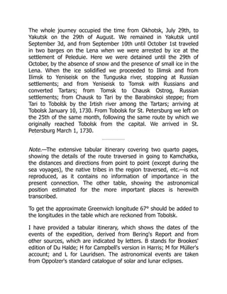
Figure 1.1 A wind turbine is affected by fluctuations in wind speed which
causes it to oscillate. We model the fluctuations as low-pass filtered noise
and the response of the construction as a linear mass-spring-damper sys-
tem. Solid lines: Simulated force, position and velocity from a stochastic
simulation of a dimensionless model. Dashed lines: Noise-free simula-
tion. The details of this model are given in Exercise 5.5. Photo credit:
CC BY-SA 4.0.
parameters in the differential equation, i.e., in f; we may want to know how
large loads the structure has been exposed to, and we may want to predict
the future production of electrical power. To answer these questions, we must
perform a statistical analysis on the time series. When we base time series
analysis on stochastic differential equations, we can use insight in the system
dynamics to fix the structure of f and maybe of g. The framework lets us
treat statistical errors correctly when estimating unknown parameters and
when assessing the accuracy with which we can estimate and predict.
Optimization and control: We may want to design a control system that
dampens the fluctuations that come from the wind. On the larger scale of the
electrical grid, we may want a control system to ensure that the power supply
meets the demand and so that voltages and frequencies are kept at the correct
values. To design such control systems optimally, we need to take into account
the nature of the disturbances that the control system should compensate for.
22.
Introduction 3
í
í
í
í
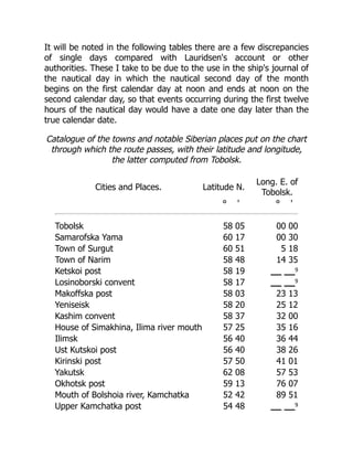
Figure 1.2 A small particle embedded in the two-dimensional flow around
a cylinder. The thin lines are streamlines, i.e., the paths a water molecule
follows, neglecting diffusion. The thick black line is a simulated random
trajectory of a particle, which is transported with the flow, but at the
same time subjected to molecular diffusion.
Motion of a Particle Embedded in a Fluid Flow
Let us examine in some more detail the origin and form of the noise term
ξt in (1.1). Figure 1.2 displays water flowing in two dimensions around a
cylinder.1
In absence of diffusion, water molecules will follow the streamlines.
A small particle will largely follow the same streamlines, but is also subject
to diffusion, i.e., random collisions with neighboring molecules which cause it
to deviate from the streamlines. Collisions are frequent but each cause only a
small displacement, so the resulting path is erratic.
In absence of diffusion, we can find the trajectory of the particle by solving
the ordinary differential equation
dXt
dt
= f(Xt).
Here, Xt ∈ R2
is the position in the plane of the particle at time t. The
function f(·) is the flow field, so that f(x) is a vector in the plane indicating
the speed and direction of the water flow at position x. To obtain a unique
solution, this equation needs an initial condition such as X0 = x0 where x0
is the known position at time 0. The trajectory {Xt : t ∈ R} is exactly a
streamline.
1The flow used here is irrotational, i.e., potential flow. Mathematically, this is convenient
even if physically, it may not be the most meaningful choice.
23.
4 StochasticDifferential Equations for Science and Engineering
To take the molecular diffusion into account, i.e., the seemingly random
motion of a particle due to collisions with fluid molecules, we add “white
noise” ξt to the equation
dXt
dt
= f(Xt) + g ξt. (1.2)
Here, g is the (constant) noise intensity, and ξt is a two-vector. The trajec-
tory in Figure 1.2 has been simulated as follows: We discretize time. At each
time step, we first advect the particle in the direction of a streamline, then we
shift it randomly by adding a perturbation which is sampled from a bivariate
Gaussian where each component has mean 0 and variance g2
h. Specifically,
Xt+h = Xt + f(Xt) h + g ξ
(h)
t where ξ
(h)
t ∼ N(0, hI).
Here, h is the time step and the superscript in ξ
(h)
t indicates that the noise term
depends on the time step, while I is a 2-by-2 identity matrix. If we let the par-
ticle start at a fixed position X0, the resulting positions {Xh, X2h, X3h, . . .}
will each be a random variable, so together they constitute a stochastic pro-
cess. This algorithm does not resolve the position between time steps; when
we plot the trajectory, we interpolate linearly.
We hope that the position Xt at a given time t will not depend too much
on the time step h as long as h is small enough. This turns out to be the case,
if we choose the noise term in a specific way, viz.
ξ
(h)
t = Bt+h − Bt,
where {Bt} is a particular stochastic process, namely Brownian motion. Thus,
we should start by simulating the Brownian motion, and next compute the
noise terms ξ
(h)
t from the Brownian motion; we will detail exactly how to
do this later. Brownian motion is key in the theory of stochastic differential
equations for two reasons: First, it solves the simplest stochastic differential
equation, dXt/dt = ξt, and second, we use it to represent the noise term in any
stochastic differential equation. With this choice of noise ξ
(h)
t , we can rewrite
the recursion with the shorthand
ΔXt = f(Xt) Δt + g ΔBt (1.3)
and since this turns out to converge as the time step h = Δt goes to zero, we
use the notation
dXt = f(Xt) dt + g dBt (1.4)
for the limit. This is our preferred notation for a stochastic differential equa-
tion. In turn, (1.3) is an Euler-type numerical method for the differential
equation (1.4), known as the Euler-Maruyama method.
If the particle starts at a given position X0 = x0, its position at a later time
t will be random, and we would like to know the probability density of the
24.
Introduction 5
positionφ(x, t). It turns out that this probability density φ(x, t) is governed
by a partial differential equation of advection-diffusion type, viz.
∂φ
∂t
= −∇ · (fφ −
1
2
g2
∇φ)
with appropriate boundary conditions. This is the same equation that governs
the concentration of particles, if a large number of particles is released and
move independently of each other. This equation is at the core of the theory of
transport by advection and diffusion, and now also a key result in the theory
of stochastic differential equations.
We can also ask, what is the probability that the particle hits the cylinder,
depending on its initial position. This is governed by a related (specifically,
adjoint) partial differential equation.
There is a deep and rich connection between stochastic differential equa-
tions and partial differential equations involving diffusion terms. This connec-
tion explains why we, in general, use the term diffusion processes for solutions
to stochastic differential equations. From a practical point of view, we can ana-
lyze PDE’s by simulating SDE’s, or we can learn about the behavior of specific
diffusion processes by solving associated PDE’s analytically or numerically.
Population Growth and State-Dependent Noise
In the two previous examples, the wind turbine and the dispersing molecule,
the noise intensity g(x) in (1.1) was a constant function of the state x. If
all models had that feature, this book would be considerably shorter; some
intricacies of the theory only arise when the noise intensity is state-dependent.
State-dependent noise intensities arise naturally in population biology, for
example. A model for the growth of an isolated bacterial colony could be:
dXt = rXt(1 − Xt/K) dt + g(Xt) dBt. (1.5)
Here, r 0 is the specific growth rate at low abundance, while K 0 is the
carrying capacity. Without noise, i.e., with g(x) ≡ 0, this is the logistic growth
model; see Figure 1.3. Dynamics of biological systems is notoriously noisy, so
we have included a noise term g(Xt) dBt and obtained a stochastic logistic
growth model. Here, it is critical that the noise intensity g(x) depends on the
abundance x; otherwise, we can get negative abundances Xt! To avoid this,
we must require that the noise intensity g(x) vanishes at the origin, g(0) = 0,
so that a dead colony stays dead. Figure 1.3 includes two realizations of the
solution {Xt} with the choice g(x) = σx. For this situation, the theory allows
us to answer the following questions:
1. How is the state Xt distributed, in particular as time t → ∞? Again,
we can pose partial differential equations of advection-diffusion type to
answer this, and the steady-state distribution can be found in closed
form. For example, we can determine the mean and variance.
25.
6 StochasticDifferential Equations for Science and Engineering
W
;
Figure 1.3 Two simulated sample paths (solid and dotted erratic curves)
of the stochastic logistic growth model (1.5) with g(x) = σx of a bac-
terial population. A noise-free simulation is included (thin black line).
Parameters are r = K = 1, σ = 0.1, X0 = 0.01. The computational time
step used is 0.001.
2. What is the temporal pattern of fluctuations in {Xt}? We shall see
that {Xt} is a Markov process, which allows us to characterize these
fluctuations. We can assess their time scale through their stochastic
Lyapunov exponent, which for this example leads to a time scale of
1/(r − σ2
/2), when the noise is weak and the process is in stochastic
steady state.
3. Does a small colony risk extinction? For this particular model with these
particular parameters, it turns out that the answer is “no”. With other
parameters, the answer is that the colony is doomed to extinction, and
for other noise structures, the answer is that there is a certain probability
of extinction, which depends on the initial size of the colony. These
questions are answered by stochastic stability theory as well as by the
theory of boundary behavior and classification.
However, before we can reach these conclusions, we must consider the
equation (1.5) carefully. We call it a stochastic differential equation, but it
should be clear from Figure 1.3 that the solutions are nowhere differentiable
functions of time. This means that we should not take results from standard
calculus for granted. Rather, we must develop a stochastic calculus which
applies to diffusion processes. In doing so, we follow in the footsteps of Kiyosi
Itô, who took as starting point an integral version of the equation (1.5), in
order to circumvent the problem that stochastic differential equations have
26.
Introduction 7
non-differentiablesolutions. The resulting Itô calculus differs from standard
calculus, most notably in its chain rule, which includes second order terms.
Overview of the Book
This book is in three parts. The core is Itô’s stochastic calculus in part 2: It
describes stochastic integrals, stochastic calculus, stochastic differential equa-
tions, and the Markov characterization of their solutions.
Before embarking on this construction, part 1 builds the basis. We first
consider molecular diffusion as a transport processes (Chapter 2); this gives
a physical reference for the mathematics. We then give a quick introduction
to measure-theoretic probability (Chapter 3) after which we study Brown-
ian motion as a stochastic process (Chapter 4). Chapter 5 concerns the very
tractable special case of linear systems such as the wind turbine (Figure 1.1).
At this point we are ready for the Itô calculus in part 2.
Finally, part 3 contains four chapters which each gives an introduction
to an area of application. This concerns estimation and time series analysis
(Chapter 10), quantifying expectations to the future (Chapter 11), stability
theory (Chapter 12) and finally optimal control (Chapter 13).
Exercises, Solutions, and Software
In science and engineering, what justifies mathematical theory is that it lets us
explain existing real-world systems and build new ones. The understanding
of mathematical constructions must go hand in hand with problem-solving
and computational skills. Therefore, this book contains exercises of differ-
ent kinds: Some fill in gaps in the theory and rehearse the ability to ar-
gue mathematically. Others contain pen-and-paper exercises while yet oth-
ers require numerical analysis on a computer. Solutions are provided at
https://github.com/Uffe-H-Thygesen/SDEbook. There, also code which re-
produces all figures is available. The computations use a toolbox, SDEtools for
R, which is available at https://github.com/Uffe-H-Thygesen/SDEtools.
There is no doubt that stochastic differential equations are becoming more
widely applied in many fields of science and engineering, and this by itself jus-
tifies their study. From a modeler’s perspective, it is attractive that our un-
derstanding of processes and dynamics can be summarized in the drift term
f in (1.1), while the noise term ξt (or Bt) manifests that our models are
always incomplete descriptions of actual systems. The mathematical theory
ties together several branches of mathematics – ordinary and partial differen-
tial equations, measure and probability, statistics, and optimization. As you
develop an intuition for stochastic differential equations, you will establish
27.
8 StochasticDifferential Equations for Science and Engineering
interesting links between subjects that may at first seem unrelated, such as
physical transport processes and propagation of noise. I have found it im-
mensely rewarding to study these equations and their solutions. My hope is
that you will, too.
C H AP T E R 2
Diffusive Transport and
Random Walks
The theory of stochastic differential equations uses a fair amount of mathe-
matical abstraction. If you are interested in applying the theory to science and
technology, it may make the theory more accessible to first consider a phys-
ical phenomenon, which the theory aims to describe. One such phenomenon
is molecular diffusion, which was historically a key motivation for the theory
of stochastic differential equations.
Molecular diffusion is a transport process in fluids like air and water and
even in solids. It is caused by the erratic and unpredictable motion of molecules
which collide with other molecules. The phenomenon can be viewed at a
microscale, where we follow the individual molecule, or at a macroscale, where
it moves material from regions with high concentration to regions with low
concentration (Figure 2.1).
The macroscale description of diffusion involves the concentration C =
C(x, t) of a substance and how it evolves in time. Here, x is the spatial position
while t is the time; the concentration measures how many molecules there are
in a given region. In this chapter, we derive and analyze the advection-diffusion
equation which governs the concentration:
∂C
∂t
= −∇ · (uC − D∇C).
In contrast, the microscale description of diffusion is that each single molecule
moves according to a stochastic process, which is governed by a stochastic
differential equation. It turns out that we can use the advection-diffusion
equation to compute the statistics of this process. In turn, we can simulate
the random motion of the molecule, which leads to Monte Carlo methods for
analyzing the advection-diffusion equation. That is, there is a precise coupling
between the microscale and the macroscale, between stochastic differential
equations and partial differential equations.
DOI: 10.1201/9781003277569-2 11
31.
12 StochasticDifferential Equations for Science and Engineering
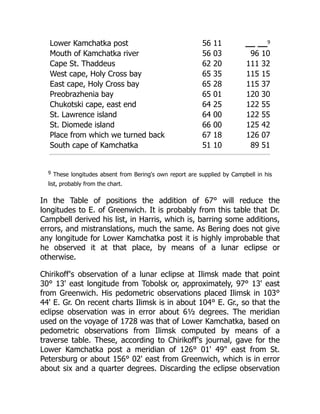
Figure 2.1 Diffusion in a container in two dimensions. Top panels: Con-
centration fields. Bottom panels: Position of 100 molecules. Left panels:
Initially, the solute is concentrated at the center. Right panels: After
some time, the solute is less concentrated. The bottom right panel also
includes the trajectory of one molecule; notice its irregular appearance.
2.1 DIFFUSIVE TRANSPORT
In this section, we model how a substance spreads in space due to molecular
diffusion. Think of smoke in still air, or dye in still water. The substance is
distributed over a one-dimensional space R. Let μt([a, b]) denote the amount
of material present in the interval [a, b] at time t. Mathematically, this μt is
a measure. We may measure the substance in terms of number of molecules
or moles, or in terms of mass, but we choose to let μt be dimensionless. We
assume that μt admits a density, which is the concentration C(·, t) of the
substance, so that the amount of material present in any interval [a, b] can be
found as the integral of the concentration over the interval:
μt([a, b]) =
b
a
C(x, t) dx.
The density has unit per length; if the underlying space had been two or three
dimensional, then C would have unit per length squared or cubed, i.e., per
area or per volume. The objective of this section is to pose a partial differential
equation, the diffusion equation (2.3), which governs the time evolution of this
concentration C.
32.
Diffusive Transport andRandom Walks 13
C
x
a b
μ
Ja
Jb
Figure 2.2 Conservation in one dimension. The total mass in the interval
[a, b] is μt([a, b]) =
b
a C(x, t) dx, corresponding to the area of the shaded
region. The net flow into the interval [a, b] is J(a) − J(b).
2.1.1 The Conservation Equation
We first establish the conservation equation
∂C
∂t
+
∂J
∂x
= 0, (2.1)
which expresses that mass is redistributed in space by continuous movements,
but neither created, lost, nor teleported instantaneously between separated
regions in space. To see that this equation holds, note that transport may
then be quantified with a flux J(x, t), which is the net amount of material
that crosses the point x per unit time, from left to right. The flux has physical
dimension “per time”. Then, the amount of material in the interval [a, b] is
only changed by the net influx at the two endpoints, i.e.,
d
dt
μt([a, b]) = J(a, t) − J(b, t).
See Figure 2.2. Assume that the flux J is differentiable in x, then
J(a, t) − J(b, t) = −
b
a
∂J
∂x
(x, t) dx.
On the other hand, since μt is given as an integral, we can use the Leibniz
integral rule to find the rate of change by differentiating under the integral
sign:
d
dt
μt([a, b]) =
b
a
∂C
∂t
(x, t) dx.
Here, we assume that C is smooth so that the Leibniz integral rule applies.
Combining these two expressions for the rate of change of material in [a, b],
we obtain: b
a
∂C
∂t
(x, t) +
∂J
∂x
(x, t)
dx = 0.
33.
14 StochasticDifferential Equations for Science and Engineering
Since the interval [a, b] is arbitrary, we can conclude that the integrand is
identically 0, or
∂C
∂t
(x, t) +
∂J
∂x
(x, t) = 0.
This is known as the conservation equation. To obtain a more compact nota-
tion, we often omit the arguments (x, t), and we use a dot (as in Ċ) for time
derivative and a prime (as in J
) for spatial derivative. Thus, we can state the
conservation equation compactly as
Ċ + J
= 0.
2.1.2 Fick’s Laws
Fick’s first law for diffusion states that the diffusive flux is proportional to the
concentration gradient:
J(x, t) = −D
∂C
∂x
(x, t) or simply J = −DC
. (2.2)
This means that the diffusion will move matter from regions of high concen-
tration to regions of low concentration. The constant of proportionality, D,
is termed the diffusivity and has dimensions area per time (also when the
underlying space has more than one dimension). The diffusivity depends on
the diffusing substance, the background material it is diffusing in, and the
temperature. See Table 2.1 for examples of diffusivities.
Fick’s first law (2.2) is empirical but consistent with a microscopic model
of molecule motion, as we will soon see. Combining Fick’s first law with the
conservation equation (2.1) gives Fick’s second law, the diffusion equation:
Ċ = (DC
)
. (2.3)
This law predicts, for example, that the concentration will decrease at a peak,
i.e., where C
= 0 and C
0. In many physical situations, the diffusivity D
is constant in space. In this case, we may write Fick’s second law as
Ċ = DC
when D is constant in space, (2.4)
i.e., the rate of increase of concentration is proportional to the spatial curva-
ture of the concentration. However, constant diffusivity is a special situation,
and the general form of the diffusion equation is (2.3).
TABLE 2.1 Examples of Diffusivities
Process Diffusivity [m2
/s]
Smoke particle in air at room temperature 2 × 10⁻⁵
Salt ions in water at room temperature 1 × 10⁻⁹
Carbon atoms in iron at 1250 K 2 × 10⁻¹¹
34.
Diffusive Transport andRandom Walks 15
Biography: Adolph Eugen Fick (1829–1901)
A German pioneer in biophysics with a background
in mathematics, physics, and medicine. Interested
in transport in muscle tissue, he used the transport
of salt in water as a convenient model system. In
a sequence of papers around 1855, he reported on
experiments as well as a theoretical model of trans-
port, namely Fick’s laws, which were derived as an
analogy to the conduction of heat.
Exercise 2.1: For the situation in Figure 2.2, will the amount of material in
the interval [a, b] increase or decrease in time? Assume that (2.4) applies, i.e.,
the transport is diffusive and the diffusivity D is constant in space.
For the diffusion equation to admit a unique solution, we need an initial
condition C(x, 0) and spatial boundary conditions. Typical boundary condi-
tions either fix the concentration C at the boundary, i.e., Dirichlet conditions,
or the flux J. In the latter case, since the flux J = uC−D∇C involves both the
concentration C and its gradient ∇C, the resulting condition is of Robin type.
In many situations, the domain is unbounded so that the boundary condition
concerns the limit |x| → ∞.
2.1.3 Diffusive Spread of a Point Source
We now turn to an important situation where the diffusion equation admits
a simple solution in closed form: We take the spatial domain to be the entire
real line R, we consider a diffusivity D which is constant in space and time,
and we assume that the fluxes vanish in the limit |x| → ∞. Consider the initial
condition that one unit of material is located at position x0, i.e.,
C(x, 0) = δ(x − x0),
where δ is the Dirac delta. The solution is then a Gaussian bell curve:
C(x, t) =
1
√
2Dt
φ
x − x0
√
2Dt
. (2.5)
Here, φ(·) is the probability density function (p.d.f.) of a standard Gaussian
variable,
φ(x) =
1
√
2π
exp(−
1
2
x2
). (2.6)
Thus, the substance is distributed according to a Gaussian distribution with
mean x0 and standard deviation
√
2Dt; see Figure 2.3. This standard devia-
tion is a characteristic length scale of the concentration field which measures
35.
16 StochasticDifferential Equations for Science and Engineering
í í
3RVLWLRQP@
RQFHQWUDWLRQP@
7LPH V
7LPH V
7LPH V
Figure 2.3 Diffusive spread. The concentration field at times t = 1, 5, 10 s
with diffusivity D = 1 m2
/s and a unit amount of material, which ini-
tially is located at the point x = 0 m.
(half the) width of the plume; recall also that for a Gaussian, the standard
deviation is the distance from the mean to inflection point. We see that length
scales with the square root of time, or equivalently, time scales with length
squared (Figure 2.4). This scaling implies that molecular diffusion is often
to be considered a small-scale process: on longer time scales or larger spatial
scales, other phenomena may take over and be more important. We will return
to this point later, in Section 2.4.
Exercise 2.2: Insert solution (2.5) into the diffusion equation and verify that
it satisfies the equation. In which sense does the solution also satisfy the initial
condition?
7LPHW
/HQJWKVFDOH
'W
Figure 2.4 Square root relationship between time and diffusive length
scale.
36.
Diffusive Transport andRandom Walks 17
Exercise 2.3: Compute the diffusive length scale for smoke in air, and for
salt in water, for various time scales between 1 second and 1 day.
Solution (2.5) is a fundamental solution (or Green’s function) with which
we may construct also the solution for general initial conditions. To see this, let
H(x, x0, t) denote the solution C(x, t) corresponding to the initial condition
C(x, 0) = δ(x − x0), i.e., (2.5). Since the diffusion equation is linear, a linear
combination of initial conditions results in the same linear combination of
solutions. In particular, we may write a general initial condition as a linear
combination of Dirac deltas:
C(x, 0) =
+∞
−∞
C(x0, 0) · δ(x − x0) dx0.
We can then determine the response at time t from each of the deltas, and
integrate the responses up:
C(x, t) =
+∞
−∞
C(x0, 0) · H(x, x0, t) dx0. (2.7)
Note that here we did not use the specific form of the fundamental solution;
only linearity of the diffusion equation and existence of the fundamental so-
lution. In fact, this technique works also when diffusivity varies in space and
when advection is effective in addition to diffusion, as well as for a much larger
class of problems. However, when the diffusivity is constant in space, we get a
very explicit result, namely that the solution is the convolution of the initial
condition with the fundamental solution:
C(x, t) =
+∞
−∞
1
(4πDt)1/2
exp
−
1
2
|x − x0|2
2Dt
C(x0, 0) dx0.
2.1.4 Diffusive Attenuation of Waves
Another important situation which admits solutions in closed form is the
diffusion equation (2.4) with the initial condition
C(x, 0) = sin kx,
where k is a wave number, related to the wavelength L by the formula kL = 2π.
In this case, the solution is
C(x, t) = exp(−λt) sin kx with λ = Dk2
. (2.8)
Exercise 2.4: Verify this solution.
Thus, harmonic waves are eigenfunctions of the diffusion operator; that
is, they are attenuated exponentially while preserving their shape. Note that
the decay rate λ (i.e., minus the eigenvalue) is quadratic in the wave number
37.
18 StochasticDifferential Equations for Science and Engineering
k. Another way of expressing the same scaling is that the half-time of the
attenuation is
T1/2 =
1
λ
log 2 =
log 2
4π2
L2
D
,
i.e., the half time is quadratic in the wave length: Twice as long waves persist
four times longer. See Figure 2.5. We recognize the square root/quadratic
relationship between temporal and spatial scales from Figure 2.4.
Recall that we used the fundamental solution (2.5) to obtain the response
of a general initial condition. We can do similarly with the harmonic solution
(2.8), although we need to add the cosines or, more conveniently, use complex
exponentials. Specifically, if the initial condition is square integrable, then it
can be decomposed into harmonics as
C(x, 0) =
1
2π
+∞
−∞
C̃(k, 0) eikx
dk,
where C̃(k, 0) is the (spatial) Fourier transform
C̃(k, 0) =
+∞
−∞
C(x, 0) e−ikx
dx.
Note that different authors use slightly different definitions of the Fourier
transform. Now, each wave component exp(ikx) is attenuated to exp(−Dk2
t+
ikx), so the Fourier transform of C(x, t) is
C̃(k, t) = C̃(k, 0) e−Dk2
t
.
í
í
[
í
í
[
Figure 2.5 Attenuation of spatial waves by diffusion. Here the diffusivity
is D = 1 and the terminal time is T = 0.01. Solid lines: At time 0, the
amplitude is 1. Dashed lines: At time T, the wave is attenuated – how
much depends on the wave number. Left panel: A long wave is attenuated
slowly. Right panel: A shorter wave is attenuated more quickly.
38.
Diffusive Transport andRandom Walks 19
We can now find the solution C(x, t) by the inverse Fourier transform:
C(x, t) =
1
2π
+∞
−∞
C̃(k, 0) e−Dk2
t+ikx
dk.
One interpretation of this result is that short-wave fluctuations (large |k|)
in the initial condition are smoothed out rapidly while long-wave fluctuations
(small |k|) persist longer; the solution is increasingly dominated by longer and
longer waves which decay slowly as the short waves disappear.
2.2 ADVECTIVE AND DIFFUSIVE TRANSPORT
In many physical situations, diffusion is not the sole transport mechanism: A
particle with higher density than the surrounding fluid will have a movement
with a downwards bias. If the fluid is flowing, then the particle will have a
tendency to follow the flow (Figure 2.6). These situations both amount to a
directional bias in the movement, so we focus on the latter.
Let the flow field be u(x, t). If we use Xt to denote the position of a fluid
element at time t, then Xt satisfies the differential equation
d
dt
Xt = u(Xt, t).
Consider again a solute which is present in the fluid, and as before let C(x, t)
denote the concentration of the solute at position x and time t. If the material
is a perfectly passive tracer (i.e., material is conserved and transported with
the bulk motion of the fluid), then the flux of material is the advective flux:
JA(x, t) = u(x, t) C(x, t).
[
[
[7
Figure 2.6 A fluid flow in one dimension which transports a substance.
The plume is advected to the right with the flow; at the same time it
diffuses out. The diffusivity is D = 1, the advection is u = 2.5, and the
terminal time is T = 4.
39.
20 StochasticDifferential Equations for Science and Engineering
If in addition molecular diffusion is in effect, then according to Fick’s first law
(2.2) this gives rise to a diffusive flux JD = −DC
. We may assume that these
two transport mechanisms operate independently, so that the total flux is the
sum of the advective and diffusive fluxes:
J(x, t) = u(x, t) C(x, t) − D(x)
∂C
∂x
(x, t),
or simply J = uC − DC
. Inserting this into the conservation equation (2.1),
we obtain the advection-diffusion equation for the concentration field:
Ċ = −(uC − DC
)
. (2.9)
A simple case is when u and D are constant, the initial condition is a Dirac
delta, C(x, 0) = δ(x − x0), where x0 is a parameter, and the flux vanishes as
|x| → ∞. Then the solution is:
C(x, t) =
1
√
4πDt
exp
−
(x − ut − x0)2
4Dt
, (2.10)
which is the probability density function of a Gaussian random variable with
mean x0 + ut and variance 2Dt. Advection shifts the mean with constant
rate, as if there had been no diffusion, and diffusion gives rise to a linearly
growing variance while preserving the Gaussian shape, as in the case of pure
diffusion (i.e., diffusion without advection). This solution is important, but
also a very special case: In general, when the flow is not constant, it will affect
the variance, and the diffusion will affect the mean.
Exercise 2.5:
1. Verify the solution (2.10).
2. Solve the advection-diffusion equation (2.9) on the real line with con-
stant u and D with the initial condition C(x, 0) = sin(kx) or, if you
prefer, C(x, 0) = exp(ikx).
2.3 DIFFUSION IN MORE THAN ONE DIMENSION
Consider again the one-dimensional situation in Figure 2.2. In n dimensions,
the interval [a, b] is replaced by a region V ⊂ Rn
. Let μt(V ) denote the amount
of the substance present in this region. This measure can be written in terms
of a volume integral of the density C:
μt(V ) =
V
C(x, t) dx.
Here x = (x1, . . . , xn) ∈ Rn
and dx is the volume of an infinitesimal volume
element. The concentration C has physical dimension “per volume”, i.e., SI
40.
Diffusive Transport andRandom Walks 21
unit m−n
, since μt(V ) should still be dimensionless. The flux J(x, t) is a vector
field, i.e., a vector-valued function of space and time; in terms of coordinates,
we have J = (J1, . . . , Jn). The defining property of the flux J is that the net
rate of exchange of matter through a surface ∂V is
∂V
J(x, t) · ds(x).
Here, ds is the surface element at x ∈ ∂V , a vector normal to the surface. The
flux J has SI unit m−n+1
s−1
. Conservation of mass now means that the rate
of change in the amount of matter present inside V is exactly balanced by the
rate of transport over the boundary ∂V :
V
Ċ(x, t) dx +
∂V
J(x, t) · ds(x) = 0, (2.11)
where ds is directed outward. This balance equation compares a volume inte-
gral with a surface integral. We convert the surface integral to another volume
integral, using the divergence theorem (the Gauss theorem), which equals the
flow out of the control volume with the integrated divergence. Specifically,
V
∇ · J dx =
∂V
J · ds.
In terms of coordinates, the divergence is ∇ · J = ∂J1/∂x1 + · · · + ∂Jn/∂xn.
Substituting the surface integral in (2.11) with a volume integral, we obtain
V
Ċ(x, t) + ∇ · J(x, t) dx = 0.
Since the control volume V is arbitrary, we get
Ċ + ∇ · J = 0, (2.12)
which is the conservation equation in n dimensions, in differential form.
Fick’s first law in n dimensions relates the diffusive flux to the gradient of
the concentration field:
J = −D∇C,
where the gradient ∇C has coordinates (∂C/∂x1, . . . , ∂C/∂xn). Often, the
diffusivity D is a scalar material constant, so that the relationship between
concentration gradient and diffusive flux is invariant under rotations. We then
say that the diffusion is isotropic. However, in general D is a matrix (or a ten-
sor, if we do not make explicit reference to the underlying coordinate system).
Then, the diffusive flux is not necessarily parallel to the gradient, and its
strength depends on the direction of the gradient. These situations can arise
when the diffusion takes place in an anisotropic material, or when the dif-
fusion is not molecular but caused by other mechanisms such as turbulence.
Anisotropic diffusion is also the standard situation when the diffusion model
does not describe transport in a physical space, but rather stochastic dynamics
in a general state space of a dynamic system.
41.
22 StochasticDifferential Equations for Science and Engineering
Fick’s second law can now be written as
Ċ = ∇ · (D∇C).
When the diffusivity is constant and isotropic, this reduces to Ċ = D∇2
C.
Here ∇2
is the Laplacian ∇2
= ∂2
∂x2
1
+ · · · + ∂2
∂x2
n
, a measure of curvature.
To take advection into account, we assume a flow field u with coordinates
(u1, . . . , un). The advective flux is now uC and the advection-diffusion equa-
tion is
Ċ = −∇ · (uC − D∇C). (2.13)
2.4 RELATIVE IMPORTANCE OF ADVECTION AND DIFFUSION
We have now introduced two transport processes, advection and diffusion,
which may be in effect simultaneously. It is useful to assess the relative im-
portance of the two.
Consider the solution (2.10) corresponding to constant advection u, con-
stant diffusion D, and the initial condition C(x, 0) = δ(x − xo). At time t, the
advection has moved the center of the plume a distance |u|t, while the diffu-
sive length scale – the half width of the plume – is
√
2Dt. These length scales
are shown in Figure 2.7 as functions of the time scale. Notice that initially,
when time t is sufficiently small, the diffusive length scale is larger than the
advective length scale, while for sufficiently large time t the advective length
scale dominates. This justifies our earlier claim that diffusion is most powerful
at small scales. The two length scales are equal when
t =
2D
u2
.
In stead of fixing time and computing associated length scales, one may fix
a certain length scale L and ask about the corresponding time scales associated
with advective and diffusive transport: The advective time scale is L/u while
7LPHW
/HQJWKVFDOHV
'LIIXVLYH
$GYHFWLYH
Figure 2.7 Advective (dashed) and diffusive (solid) length scale as func-
tion of time scale for the dimensionless model with u = D = 1.
42.
Diffusive Transport andRandom Walks 23
the diffusive time scale is L2
/2D. We define the Péclet number as the ratio
between the two:
Pe = 2
Diffusive time scale
Advective time scale
=
Lu
D
.
It is common to include factor 2 in order to obtain a simpler final expression,
but note that different authors may include different factors. Regardless of the
precise numerical value, a large Péclet number means that the diffusive time
scale is larger than the advective time scale. In this situation, advection is a
more effective transport mechanism than diffusion at the given length scale;
that is, the transport is dominated by advection. Conversely, if the Péclet
number is near 0, diffusion is more effective than advection at the given length
scale. Such considerations may suggest to simplify the model by omitting the
least significant term, and when done cautiously, this can be a good idea.
The analysis in this section has assumed that u and D were constant.
When this is not the case, it is customary to use “typical” values of u and D
to compute the Péclet number. This can be seen as a useful heuristic, but can
also be justified by the non-dimensional versions of the transport equations,
where the Péclet number enters. Of course, exactly which “typical values”
are used for u and D can be a matter of debate, but this debate most often
affects digits and not orders of magnitude. Even the order of magnitude of the
Péclet number is a useful indicator if the transport phenomenon under study
is dominated by diffusion or advection.
Example 2.4.1 Consider the advection-diffusion equation (2.13) in two di-
mensions, where the flow u(x) is around a cylinder. We non-dimensionalize
space so that the cylinder is centered at the origin and has radius 1, and non-
dimensionalize time so that the flow velocity far from the cylinder is 1. Then,
the flow is, in polar coordinates (r, θ) with x = r cos θ, y = r sin θ,
ur(r, θ) = (1 − r−2
) cos θ, uθ = −(1 + r−2
) sin θ.
This is called irrotational flow in fluid mechanics (Batchelor, 1967). A unit of
material is released at time t = 0 at position x = −3, y = −0.5. We solve the
advection-diffusion equation for t ∈ [0, 2.5] for three values of the diffusivity
D: D = 1, D = 0.1, and D = 0.01, leading to the three Péclet numbers 1, 10,
and 100. Figure 2.8 shows the solution at time t = 2.5 for the three Péclet
numbers. Notice how higher Péclet numbers (lower diffusivity D) imply a more
narrow distribution of the material.
2.5 THE MOTION OF A SINGLE MOLECULE
We can accept Fick’s first equation as an empirical fact, but we would like
to connect it to our microscopic understanding. In this section, we present a
caricature of a microscopic mechanism which can explain Fickian diffusion:
Each individual molecule moves in an erratic and unpredictable fashion, due
43.
24 StochasticDifferential Equations for Science and Engineering
4 2 0 2 4
4
2
0
2
4
4 2 0 2 4
4
2
0
2
4
4 2 0 2 4
4
2
0
2
4
Figure 2.8 Concentrations C(x, t = 2.5) from Example 2.4.1, for flow
around a cylinder with diffusivities leading to different Péclet numbers.
Left panel: Pe = 1. Center panel: Pe = 10. Right panel: Pe = 100. In each
panel, the grayscale represents concentration relative to the maximum
concentration.
í
7LPHQV@
3RVLWLRQμP@
í
í
7LPHQV@
3RVLWLRQμP@
Figure 2.9 A random walk model of molecular motion. Left: A close-up
where individual transitions are visible. Right: A zoom-out where the
process is indistinguishable from Brownian motion.
to the exceedingly large number of collisions with other molecules, so that
only a probabilistic description of its trajectory is feasible. This phenomenon
is called Brownian motion.
Let Xt ∈ R denote the position at time t of a molecule, e.g., smoke in air,
still considering one dimension only. At regularly spaced points of time, a time
step h apart, the molecule is hit by an air molecule which causes a displacement
±k. This happens independently of what has happened previously (Figure
2.9).1
1Physcially, collisions cause changes in velocity rather than position, but the simple
picture is more useful at this point. We can argue that the velocity decays to 0 due to
viscous friction and that the molecule drifts a certain distance during this decay. The simple
model was used by Einstein (1905); extensions that take the velocity process into account
were the Langevin (1908) equation and the Ornstein-Uhlenbeck process (Uhlenbeck and
Ornstein, 1930) (Section 5.10).
44.
Diffusive Transport andRandom Walks 25
Biography: Robert Brown (1773–1858)
A Scottish botanist who in 1827 studied pollen im-
mersed in water under a microscope and observed
an erratic motion of the grains. Unexplained at
the time, we now attribute the motion to seem-
ingly random collision between the pollen and wa-
ter molecules. The physical phenomenon and its
mathematical model are named Brownian motion,
although many other experimentalists and theoreti-
cians contributed to our modern understanding of
the phenomenon.
In summary, the position {Xt : t ≥ 0} is a random walk:
Xt+h =
⎧
⎨
⎩
Xt + k w.p. (with probability) p,
Xt w.p. 1 − 2p,
Xt − k w.p. p.
.
Here, p ∈ (0, 1
2 ] is a parameter. The displacement in one time step, Xt+h −Xt,
has mean 0 and variance 2k2
p. Displacements over different time steps are
independent, so the central limit theorem applies. After many time steps, the
probability distribution of the displacement Xnh will be well approximated
by a Gaussian with mean 0 and variance 2k2
pn:
Xnh ∼ N(0, 2k2
pn). (2.14)
That is, Xnh will (approximately) have the probability density function
1
2k2pn
· φ(x/ 2k2pn),
where φ is still the p.d.f. of a standard Gaussian variable from (2.6). Next,
assume that we release a large number N of molecules at the origin, and that
they move independently. According to the law of large numbers, the number
of molecules present between x1 and x2 at time nh will be approximately
N
x2
x1
1
2k2pn
· φ(x/ 2k2pn) dx.
Notice that this agrees with equation (2.5), assuming that we take N = 1,
D = k2
p/h and t = nh.
We see that our cartoon model of molecular motion is consistent with the
results of the diffusion equation, if we assume that
45.
26 StochasticDifferential Equations for Science and Engineering
Biography: Albert Einstein (1879–1955)
In his Annus Mirabilis, Einstein (1905) published
not just on the photoelectric effect and on special
relativity, but also on Brownian motion as the result
of molecular collisions. His work connected pressure
and temperature with the motion of molecules, gave
credibility to statistical mechanics, and estimated
the size of atoms. Soon confirmed in experiments
by Jean Perrin, this work ended the debate whether
atoms really exist.
1. molecules take many small jumps, i.e., h and k are small, so that the
Central Limit Theorem is applicable at any length and time scale that
our measuring devices can resolve, and
2. there is a large number of molecules present and they behave indepen-
dently, so that we can ignore that their number will necessarily be inte-
ger, and ignore its variance.
Both of these assumptions are reasonable in many everyday situations
where molecular systems are observed on a macroscale, for example, when
breathing or making coffee.
To simulate the motion of a single molecule, if we only care about the
displacements after many collisions, we may apply the approximation (2.14)
recursively to get
Xt − Xs ∼ N(0, 2D(t − s)), when t s.
Here we have assumed that the steps in time and space are consistent with
the diffusivity, i.e., D = k2
p/h. This process {Xt} with independent and
stationary Gaussian increments is called (mathematical) Brownian motion.
Note that, physically, these properties should only hold when the time lag t−s
is large compared to the time h between molecular collisions, so mathematical
Brownian motion is only an appropriate model of physical Brownian motion
at coarse scale, i.e., for large time lags t − s. Mathematical Brownian motion
is a fundamental process. It is simple enough that many questions regarding
its properties can be given explicit and interesting answers, and we shall see
several of these later, in Chapter 4.
In many situations, we choose to work with standard Brownian motion,
where we take 2D = 1 so that the displacement Bt+h − Bt has variance equal
to the time step h. When time has the physical unit of seconds s, notice that
this means that Bt has the physical unit of
√
s!
46.
Diffusive Transport andRandom Walks 27
2.6 MONTE CARLO SIMULATION OF PARTICLE MOTION
The previous section considered diffusion only. To add advection, the mi-
croscale picture is that each particle is advected with the fluid while subject
to random collisions with other molecules which randomly perturb the parti-
cle. Thus, each particle performs a biased random walk. When the diffusivity
D and the flow u are constant in space and time, the Gaussian solution (2.10)
to the advection-diffusion equation applies. Then, a random walk model that
is consistent with the advection-diffusion equation is to sample the increments
ΔX = Xt − Xs from a Gaussian distribution
ΔX ∼ N(u · (t − s), 2D(t − s)).
Now what if the flow u = u(x, t) varies in space and time? To simulate the
trajectory of a single particle, it seems to be a reasonable heuristic to divide
the time interval [0, T] into N subintervals
0 = t0, t1, . . . , tN = T.
We first sample X0 from the initial distribution C(·, 0). Then, we sample the
remaining trajectory recursively: At each sub-interval [ti, ti+1], we approxi-
mate the flow field with a constant, namely u(Xti
, ti). This gives us:
Xti+1 ∼ N(Xti + u(Xti ) · Δti, 2D · Δti), (2.15)
where Δti = ti+1 −ti. It seems plausible that, as the time step in this recursion
goes to 0, this approximation becomes more accurate so that the p.d.f. of Xt
will approach the solution C(·, t) to the advection-diffusion equation (2.9).
This turns out to be the case, although we are far from ready to prove it.
Example 2.6.1 (Flow past a cylinder revisited) Example 2.4.1 and Fig-
ure 2.8 present solutions of the advection-diffusion equation for the case where
the flow goes around a cylinder. In the introduction, Figure 1.2 (page 3) show
a trajectory of a single molecule in the same flow. This trajectory is simulated
with the recursion (2.15), using a Péclet number of 200.
The Monte Carlo method, we have just described simulates the motion of
single molecules, chosen randomly from the ensemble. Monte Carlo simulation
can be used to compute properties of the concentration C, but can also answer
questions that are not immediately formulated using partial differential equa-
tions; for example, concerning the time a molecule spends in a region. Monte
Carlo methods are appealing in situations where analytical solutions to the
partial differential equations are not available, and when numerical solutions
are cumbersome, e.g., due to irregular geometries. Monte Carlo methods can
also be useful when other processes than transport are active, for example,
when chemical reactions take place on or between the dispersing particles.
47.
28 StochasticDifferential Equations for Science and Engineering
2.7 CONCLUSION
Diffusion is a transport mechanism, the mathematical model of which involves
the concentration field and the flux. Fick’s laws tell us how to compute the flux
for a given concentration field, which in turn specifies the temporal evolution
of the concentration field. This is the classical approach to diffusion, in the
sense of 19th century physics.
A microscopic model of diffusion involves exceedingly many molecules
which each move erratically and unpredictably, due to collisions with other
molecules. This statistical mechanical image of molecular chaos is consistent
with the continuous fields of classical diffusion, but brings attention to the mo-
tion of a single molecule, which we model as a stochastic process, a so-called
diffusion process. The probability density function associated with a single
molecule is advected with the flow while diffusing out due to unpredictable
collisions, in the same way the overall concentration of molecules spreads.
We can simulate the trajectory of a diffusing molecule with a stochastic re-
cursion (Section 2.6). This provides a Monte Carlo particle tracking approach
to solving the diffusion equation, which is useful in science and engineer-
ing: In each time step, the molecule is advected with the flow field but per-
turbed randomly from the streamline, modeling intermolecular collisions. This
Monte Carlo method is particular useful in high-dimensional spaces or complex
geometries where numerical solution of partial differential equations is difficult
(and analytical solutions are unattainable).
Molecular diffusion is fascinating and relevant in its own right, but has even
greater applicability because it serves as a reference and an analogy to other
modes of dispersal; for example, of particles in turbulent flows, or of animals
which move unpredictably (Okubo and Levin, 2001). At an even greater level
of abstraction, a molecule moving randomly in physical space is a archetypal
example of a dynamic system moving randomly in a general state space. When
studying such general systems, the analogy to molecular diffusion provides not
just physical intuition, but also special solutions, formulas and even software.
With the Monte Carlo approach to diffusion, the trajectory of the diffus-
ing molecule is the focal point, while the classical focal points (concentrations,
fluxes, and the advection-diffusion equation that connect them) become sec-
ondary, derived objects. This is the path that we follow from now on. In the
chapters to come, we will depart from the physical notion of diffusion, in or-
der to develop the mathematical theory of these random paths. While going
through this construction, it is useful to have Figure 2.1 and the image of
a diffusing molecule in mind. If a certain piece of mathematical machinery
seems abstract, it may be enlightening to consider the question: How can this
help describe the trajectory of a diffusing molecule?
48.
Diffusive Transport andRandom Walks 29
Factbox: [The error function] The physics literature often prefers the “er-
ror function” to the standard Gaussian cumulative distribution function.
The error function is defined as
erf(x) =
2
√
π
x
0
e−s2
ds,
and the complementary error function is
erfc(x) = 1 − erf(x) =
2
√
π
∞
x
e−s2
ds.
These are related to the standard Gaussian distribution function Φ(x) by
erfc(x) = 2 − 2Φ(
√
2x), Φ(x) = 1 −
1
2
erfc(x/
√
2).
erf(x) = 2Φ(
√
2x) − 1, Φ(x) =
1
2
+
1
2
erf(x/
√
2).
2.8 EXERCISES
Exercise 2.6:
1. Solve the diffusion equation (2.4) on the real line with a “Heaviside step”
initial condition
C(x, 0) =
0 when x 0,
1 when x 0.
.
Use boundary conditions limx→+∞ C(x, t) = 1 and limx→−∞ C(x, t) =
0.
Hint: If you cannot guess the solution, use formula (2.7) and manipulate
the integral into a form that resembles the definition of the cumulative
distribution function.
2. Consider the diffusion equation (2.4) on the positive half-line x ≥ 0
with initial condition C(x, 0) = 0 and boundary conditions C(0, t) = 1,
C(∞, t) = 0.
Hint: Utilize the solution of the previous question, and the fact that in
that question, C(0, t) = 1/2 for all t 0.
Exercise 2.7: It is useful to have simple bounds on the tail probabilities in
the Gaussian distribution, such as (Karatzas and Shreve, 1997):
x
1 + x2
φ(x) ≤ 1 − Φ(x) ≤
1
x
φ(x).
49.
30 StochasticDifferential Equations for Science and Engineering
which hold for x ≥ 0. Here, as always, Φ(·) is the c.d.f. of a standard Gaussian
variable X ∼ N(0, 1), so that 1 − Φ(x) = P(X ≥ x) =
∞
x
φ(y) dy with φ(·)
being the density, φ(x) = 1
√
2π
e− 1
2 x2
. A useful consequence is
1 − Φ(x) = φ(x) · (x−1
+ O(x−3
)).
1. Plot the tail probability 1 − Φ(x) for 0 ≤ x ≤ 6. Include the upper and
lower bound. Repeat, in a semi-logarithmic plot.
2. Show that the bounds hold. Hint: Show that the bounds hold as x → ∞,
and that the differential version of the inequality holds for x ≥ 0 with
reversed inequality signs.
Exercise 2.8: Consider pure diffusion in n 1 dimensions with a scalar
diffusion D, and a point initial condition C(x, 0) = δ(x − x0), where x ∈ Rn
and δ is the Dirac delta in n dimensions. Show that each coordinate can be
treated separately, and thus, that the solution is a Gaussian in n dimensions
corresponding to the n coordinates being independent, i.e.,
C(x, t) =
n
i=1
1
√
2Dt
φ
ei(x − xo)
√
2Dt
=
1
(4πDt)n/2
exp
−
1
2
|x − x0|2
2Dt
,
where ei is the ith unit vector.
50.
C H AP T E R 3
Stochastic Experiments
and Probability Spaces
To build the theory of stochastic differential equations, we need precise prob-
abilistic arguments, and these require an axiomatic foundation of probability
theory. This foundation is measure-theoretic and the topic of this chapter.
In science and engineering, probability is typically taught elementary, i.e.,
without measure theory. This is good enough for many applications, but it
does not provide firm enough ground for more advanced topics like stochas-
tic differential equations. One symptom of this is the existence of paradoxes
in probability: Situations, or brain teasers, where different seemingly valid
arguments give different results. Another symptom is that many elementary
introductions to probability fail to give precise definitions, but in stead only
offer synonyms such as “a probability is a likelihood”.
The measure-theoretic approach to probability constructs a rigorous the-
ory by considering stochastic experiments and giving precise mathematical
definitions of the elements that make up such experiments: Sample spaces,
realizations, events, probabilities, random variables, and information. To gain
intuition, we consider simple experiments such as tossing coins or rolling dice,
but soon we see that the theory covers also more complex experiments such
as picking random functions.
At the end, we reach a construction which is consistent with the elementary
approach, but covers more general settings. Therefore, there is no need to “un-
learn” the elementary approach. The measure theoretic approach may seem
abstract, but it gives precise mathematical meaning to concepts that not many
people find intuitive. Once one has become familiar with the concepts, they
can even seem natural, even if they are still technically challenging. A final
argument in favor of the measure-theoretic approach is that the mathematical
literature on stochastic differential equations is written in the language of
measure theory, so the vocabulary is necessary for anyone working in this
field, even if one’s interest is applications rather than theory.
DOI: 10.1201/9781003277569-3 31
51.
32 StochasticDifferential Equations for Science and Engineering
Ω
A
ω
Figure 3.1 In a stochastic experiment, Chance picks an outcome ω from
the sample space Ω. An event A is a subset of Ω and occurs or is true if
ω ∈ A. For the outcome ω in the figure, the event A did not occur.
3.1 STOCHASTIC EXPERIMENTS
The most fundamental concept in probability theory is the stochastic experi-
ment. This is a mathematical model of real-world experiments such as rolling
a die and observing the number of eyes.
Mathematically, a stochastic experiment involves a set containing all possi-
ble outcomes: The sample space Ω. We let ω denote an element in Ω; we call ω
an outcome or a realization. For the die experiment, we set Ω = {1, 2, 3, 4, 5, 6}.
The stochastic experiment is that some mechanism, or the Goddess of Chance,
selects one particular outcome ω from the sample space Ω (Figure 3.1).
A few other examples:
Statistical models: Statistical methods for data analysis are justified by
postulating that the data has been produced by a stochastic experiment. For
example, we may weigh an object n times, obtaining measurements y1, . . . , yn,
and postulating yi = μ + ei. Here, μ is the (unknown) true weight of the
object and ei is the ith measurement error. We take the sample space to be
Ω = Rn
and identify the outcome ω ∈ Ω with the measurement errors, i.e.,
ω = (e1, . . . , en).
Monte Carlo simulation: In computer simulations of stochastic ex-
periments, we rely on a random number generator which, ideally, produces
an infinite series of independent and identically distributed numbers {Zi ∈
R : i ∈ N}. Hence, the sample space is the set of sequences of real numbers,
Ω = RN
. If we take into account that computers only produce pseudo-random
numbers, we may identify the realization ω with the seed of the random num-
ber generator; this allows to repeat the stochastic experiment, picking the
same realization ω.
Diffusion and Brownian motion: In Chapter 2, we considered the
experiment of releasing a large number of molecules; say, dye in water. A
stochastic experiment is to pick one random molecule and record how its po-
sition changes in time. A mathematical model of this, in one dimension, is
Brownian motion (Chapter 4), where the sample space is Ω = C(R̄+, R),
the set of continuous real-valued functions defined on [0, ∞). We identify the
52.
Stochastic Experiments andProbability Spaces 33
randomly chosen continuous function ω ∈ Ω with the trajectory of the
molecule {Bt : t ≥ 0}.
Once the sample space Ω is defined, we next need events. Events are state-
ments about the outcome, such as “The die showed an even number” or “the
molecule hits x = 1 before time t = 1”. Once the experiment has been per-
formed, the statement is either true or false. Mathematically, an event A is
a subset of Ω containing those outcomes for which the statement is true. For
example:
• For the die experiment, the statement “The die shows an even number”
is the event {2, 4, 6}.
• For the linear regression model, an event is a subset of Rn
. One example
is the event “all the measurement errors are positive”, corresponding to
Rn
+.
This brings us to probabilities: The point of the stochastic model is to as-
sign probabilities to each event. For the die-tossing experiment, if the die is
fair, then P({2, 4, 6}) = 1/2, for example. This probability can be interpreted
in different ways. The frequentist view is that if we toss the die repeatedly, we
will eventually observe that the die has shown 2, 4 or 6 in half the tosses. The
subjective Bayesian view is that we subjectively believe the event {2, 4, 6} to
be as probable as the alternative, {1, 3, 5}, and aims for consistency in such
subjective beliefs. From an applied and pragmatic point of view, in some sit-
uations the frequentist view is justified, while in others the Bayesian view is
more appropriate; even other interpretations exist. Fortunately, the mathe-
matical construction in the following applies regardless of the interpretation.
Now the vocabulary is in place – sample space, outcomes, events, prob-
abilities – we need to specify the mathematical properties of these objects.
First, which events do we consider? For the example of the die, it is simple:
Any subset of Ω is allowed, including the empty set and Ω itself. Moreover,
if the die is fair, the probability of an event depends only on the number of
elements in it, P(A) = |A|/|Ω|.
For the statistical model, we could start by trying to make an event out of
each and every subset A of Rn
. In an elementary course on probability and
statistics, we would maybe postulate a probability density function f(e) for
each measurement error and claim independence such that
P(A) =
A
f(e1) · · · f(en) de1 · · · den.
Unfortunately, it turns out that there are subsets A of Rn
that are so patho-
logical that this integral is not defined – even for n = 1 and regardless of
how regular f is. You can accept this as a curious mathematical fact, or you
can look up the “Vitali set” in (Billingsley, 1995) or on Wikipedia. We need
53.
34 StochasticDifferential Equations for Science and Engineering
to exclude such “non-measurable” subsets of Rn
: They do not correspond to
events.
In elementary probability and statistics, we tend to ignore non-measurable
subsets of Rn
, which have little relevance in applications. However, for more
complicated sample spaces Ω, which appear in the study of stochastic processes
and in particular stochastic differential equations, this difficulty cannot be
ignored: Not all subsets of the sample space can be events, and we often need
careful analysis to determined which ones are.
When not every set A ⊂ Ω can be an event, which ones should be? Some
events are required for the theory to be useful. For example, in the scalar
case Ω = R, we want intervals to correspond to events, so that the statement
ω ∈ [a, b] is an event for any a and b. Moreover, it is imperative that our
machinery of logic works: If A is an event, then the complementary set Ac
must also be an event, so that the statement “not A” is valid. Next, if also
B is an event, then the intersection A ∩ B must also be an event, so that the
statement “A and B” is valid. More generally, in stochastic processes we often
consider infinite sequences of events, for instance when analyzing convergence.
So if {Ai : i ∈ N} is a sequence of events, then the statement “for each integer
i, the statement Ai holds” should be valid. In terms of subsets of sample space
Ω, this means that A1 ∩ A2 ∩ . . . must be an event.
Let F denote the collection of events which we consider. Mathematically
speaking, the requirements on F that we have just argued for, means that F
is a σ-algebra:
Definition 3.1.1 (σ-algebra of events) Given a sample space Ω, a σ-
algebra F of events is a family of subsets of Ω for which:
1. The certain event is included, Ω ∈ F.
2. For each event A ∈ F, the complementary set Ac
is also an event,
Ac
∈ F.
3. Given a sequence of events {Ai ∈ F : i ∈ N}, it is an event that all Ai
occur, i.e., ∩iAi ∈ F.
Given a sequence of events {Ai ∈ F : i ∈ N}, also the union ∪iAi is an event.
Exercise: Verify this!. We often say, for short, that σ-algebras are characterized
by being closed under countable operations of union and intersection.
Example 3.1.1 (The Borel algebra) A specific σ-algebra which we will
encounter frequently in this book, is related to the case Ω = R. We previously
argued that the intervals [a, b] should be events for the theory to be useful in
many situations. The smallest σ-algebra which contains the intervals is called
the Borel-algebra and denoted B(R) or simply B.
The Borel algebra contains all open sets and all closed sets, as well as many
others. This collection of sets is large enough to contain the sets one encoun-
ters in practice, and the fact that the Vitali set and other non-Borel sets exist
is more an excitement to mathematicians than a nuisance to practitioners.
54.
Stochastic Experiments andProbability Spaces 35
Biography: Félix Édouard Justin Émile Borel (1871–1956)
The French mathematician Borel was one of the
leading figures in the development of measure the-
ory. He applied measure theory to real functions of
real variables, as well as to the foundations of prob-
ability. He was also politically active, argued for a
united Europe, was Minister of the Navy, and was
imprisoned during World War II for assisting the
Resistance.
In the case Ω = Rn
, we require F to include (hyper)rectangles of the form
(a1, b1) × (a2, b2) × . . . × (an, bn), for ai, bi ∈ R and also use the name Borel-
algebra, B(Rn
), for the smallest σ-algebra that contains these hyper-rectangles.
More generally, if Ω is a topological space (i.e., we have defined a system of
open subsets of Ω), then the Borel algebra on Ω is the smallest σ-algebra of
subsets of Ω that contain all the open sets.
It is important to notice that for a given sample space Ω, there can be
several systems of events F. In many applications there is an obvious choice,
but in general, to specify a stochastic experiment, we must state not only
what can happen (i.e., Ω) but also which questions we can ask (i.e., F).
Having outcomes and events in place, we need to assign a probability P(A)
to each event A ∈ F. The way we do this must be consistent:
Definition 3.1.2 (Probability measure) A measure P is a map F →
[0, ∞] which is countably additive, i.e.: P(∪iAi) =
i P(Ai) whenever
A1, A2, . . . are mutually exclusive events (Ai ∩ Aj = ∅ for i = j). A prob-
ability measure is a measure for which P(Ω) = 1.
This definition explains why we call the sets in F measurable: F consists
exactly of those sets, for which the measure P(A) is defined. Notice that
probability is additive only for countable collections of sets, just as the σ-
algebra F must only be closed under countable unions of sets.
An event with probability 0 is called a null event. Conversely, if an event
has probability 1, then we say that this event occurs almost surely (a.s.) or
with probability 1 (w.p. 1).
Example 3.1.2 Consider the uniform distribution on [0, 1); i.e., Ω = [0, 1),
F is the Borel algebra on Ω, and probability corresponds to length, P([a, b]) =
b−a for 0 ≤ a ≤ b 1. Now, the rational numbers form a countable set Q, so
the set A = Ω∩Q is measurable and has measure P(A) = 0: When sampling a
real number uniformly from [0, 1), the probability of getting a rational number
is 0. At the same time, the rationals are dense in [0, 1) (every real number can
true Anadyr withoutseeing it. The coast lines are essentially those of Bering. Beyond the
basins of the Kolyma and Anadyr is marked Terre inconnue; a small supplement in the
north-east corner of the map, on half the scale of the map, represents the north-east
extreme of Asia as delineated by Bering. This little supplement is of considerable interest
as it gives fuller information than that which appears on the original publication of Du
Halde, perhaps from a more modern version of Bering's chart, as previously suggested.
Several names appear for the first time in cartographic history, upon this map.
Preobrazhenia Bay; Bolshoia River falling into Holy Cross Bay, and the Isle de St.
Diomide are among these. The Island of St. Demetrius is omitted, as well as its name.
The Island of St. Diomide is placed about on a line between East Cape and Cape
Chukotski, to the westward of the meridian of East Cape. There is a discrepancy
averaging about five minutes in latitude and longitude between the positions on this map
and those on the second version of the Bering manuscript charts. But in the main these
differences are, I suspect, merely due to carelessness in copying, and the general
harmony between the two leads to the belief that the D'Anville outline for this region was
based on the second version of the manuscript.
The differences of position for points on this part of the coast are numerous. I have
noted them in the comparative table of positions herewith. They may be chiefly owing to
slips in transferring from the Mercator to the Polyconic projection; but some of them are
due to new information, probably derived from the surveyors of the second expedition.
Bering island appears on the map, in about its proper place, though Copper island is not
indicated, nor are any of the Aleutians shown. I suspect this is the first publication of a
cartographic kind on which Bering island is laid down, as the map of the Imperial
Academy of Sciences, embodying the geographical results of Bering's Voyage to the
coast of America, was not engraved until a year later, while De L'Isle's of 1752 does not
contain them.
The island between Cape Shelaginski and East Cape off the northern coast, on Bering's
map, is omitted by D'Anville. The Kamchatkan peninsula in latitude 56° is represented to
have a width of 180 miles, while Bering made it 270 miles.
A most important contribution to the subject appeared in Müller's Historical Collections
known as the Sammlung Russische Geschichte and published at St. Petersburg
(Kayserl. Academie der Wissenschaften, 1732-64. 8°. Nine volumes.) Des dritten Bandes
(erstes, zweytes und drittes Stück, pp. 1-304, 1758) contains the original account of the
57.
Russian Voyages towardAmerica from which the work of Jefferys has, with some errors
and omissions, been translated. As far as regards Bering's first voyage, there is only one
error of consequence made by Jefferys, which will be noted in its place. This book is
extremely rare, and the only copy in America which I have been able to find after much
enquiry, is in the library of the Smithsonian Institution.
The first volume of this series has the title
Eröffnung eines Vorschlages zu Verbesserung der Russischen Historie
Durch den Druck eines Stückweise herauszugebenden Sammelungen
von allerly zu den Umstanden und Begebenheiten dieses Reichs
gehorigen Nachrichten. St. Petersburg, bey der Keyserl. Academie der
Wissenschaften, 1732.
The succeeding volumes have the running title Sammlung Russische Geschichte with
the number of the parts subjoined but no other title-page.
The account of the Russian Voyages is stated by Müller to have been prepared at the
direction of the Empress and endorsed by the Academy of Sciences. It contains
invaluable material on the early explorations, which, if it had not been for Müller's
painstaking researches, would have been totally lost, as the archives of Yakutsk from
whence the data were derived by Müller were subsequently destroyed by fire. The errors
which occur in it are chiefly due to Müller's endeavor to utilize the inexact geographical
data of the Promyschleniks and Cossacks by combining them with the less detailed but
more precise observations of later observers. In this attempt he added many valuable
details to the charts, but at the same time introduced several errors. The exaggerated
distances reported by the first explorers who were unable to correct their estimates by
observations of precision, distort those parts of the map due to their reports. The
peninsula of Aliaska becomes hugely exaggerated as does the Shelagskoi promontory on
the Arctic Sea. But no unprejudiced person can read Müller's account without perceiving
his great caution in accepting unreservedly these imperfect contributions, the really
important additions which he made to cartography, the preciousness of the facts which
he rescued from oblivion, and his desire to be fair to everybody.
The insinuations of malice and of a desire to injure Bering by means of this account
given by Müller, which Lauridsen attributes to the latter, appear to be entirely the product
of a suspicious temperament and an excited imagination. Certainly I have seen nothing
anywhere cited which lends to such suspicions any tint of probability. The facts cited in
58.
support of themcan easily be otherwise explained, if one desires to view the subject
judicially, and for the most part are not quite thoroughly understood by the Danish
author.
One error upon which the latter lays great stress, is due to a manipulation of the record,
originated or at least adopted by Bering himself, and which is incorporated in the map
and report which all authors agree proceeded directly from Bering's own hand.
The next map of importance was issued by the Imperial Academy of Sciences, St.
Petersburg in 1754. It was made under the inspection of Gerhard Friedrich, Staatsrath
von Müller, who revised and corrected it subsequently, when an edition dated 1758 was
issued. This map comprised the geographical results of the great Siberian expedition
sent out by the Russian government; of Bering's voyages; and of the records of the
hunters (Promishleniks) and traders in northeastern Siberia preserved in the archives of
Yakutsk. The sources of this map are fully explained by Müller in the Russian
Discoveries (Jefferys' translation, p. 108 et seq.). I have not been able to examine a
copy of the original map, and have therefore relied on the English version of it which is
to be found in Jefferys' translation, second edition, London, 1764.
Among the improvements introduced on this map may be specified, the correction of the
shores of the Okhotsk Sea, and Gulf of Penjina, the correcter location of the mouth of
the Anadyr river and its estuary, the introduction of the results of the voyages of
Gvosdeff, Bering and Chirikoff to the northwest coast of America, and a multitude of
details relating to northeastern Siberia. The island of St. Deomid (Diomede) is not
represented though its name appears on the 65th parallel in Bering Strait. The island
may have been on the original map and carelessly omitted by Jefferys' engraver on his
copy. Among the errors, or rather mistaken hypotheses of others, which are suggested in
this map by dotted lines, are the extension westward to 174° E. of Greenwich, of the
peninsula of Aliaska which is also given a wholly uncalled-for width; and the northward
extension of the coast on each side of Bering Strait. In the former case the cartographer
was misled by the errors of the map of Bering and Chirikoff's last voyage and rumors
reported by other navigators; and in the second case he followed Bering in adopting an
erroneous position and exaggerated form for the coast eastward from Koliuchin Bay, due
to the uncorrected sketches of the Cossacks and traders. The northern extension of the
American coast opposite, was purely hypothetical and for this Müller must be held
responsible. Many of the western Aleutians are exaggerated in size and erroneous in
59.
position but thechart of Bering's last voyage, and the exaggerated reports of the
hunters who followed him, must be held responsible for this, in the main.
The work in which this chart appears is largely derived from Müller's Sammlung
russische geschichte, St. Petersburg, 1758, vol. iii, Parts I-III (cf. antea). The first
edition is entitled, according to bibliographies:
Voyages from Asia to America for completing the discoveries of the
northwest coast of America. A summary of voyages made by the
Russians on the frozen sea. From the high Dutch of S[taatsrath]. Muller
by T. Jefferys. London: T. Jefferys, 1761. lxvi, 76 pp. 4°, with four
maps.
The second edition which is that referred to in this paper is entitled
Voyages from Asia to America, for completing the discoveries of the
northwest coast of America. To which is prefixed, a summary of the
Voyages made by the Russians on the Frozen Sea, in search of a
northeast passage. Serving as an explanation of a map of the Russian
discoveries, published by the Academy of Sciences at Petersburgh,
[etc.] London: T. Jefferys, 1764, viii, 120 pp. 4°, four maps.
A French translation by Dumas, with the author's initials misprinted G. P. instead of G. F.,
was printed at Amsterdam in 1766. It consisted of two volumes, 18mo, with a map. A
Danish translation, by Morten Hallager, was issued at Copenhagen in 1784, as a portion
of a volume relating to northern explorations. Bibliographers seem to have been puzzled
by the discrepancy of initials, not recognizing that the S. in Jefferys' volume stood for a
title and not a name. Another work important in its collection of facts bearing upon the
general question of the explorations eastward by the Russians, was published by the
archdeacon of Wilts, Rev. William Coxe in 1780. This was followed by a second edition
during the same year. A third edition accompanied by a Supplement of 57 pages was
printed in 1787 and a fourth in 1803. There were two apparently distinct translations of
the book printed at Paris in 1781, and a German edition at Frankfurt and Leipzig in 1783.
The third edition which is the best and most correct appeared both in octavo and quarto
form, and is that to which reference is made in this paper. It is entitled:
Account of the Russian discoveries between Asia and America. To
which are added the Conquest of Siberia, and the history of the
60.
transactions and commercebetween Russia and China, [etc.]. London:
T. Cadell, 1787.
410 pp. 8° [or 4°] with four charts and one plate; to which is added, consecutively
paged:
A comparative view of the Russian discoveries with those made by
Captains Cook and Clerke, and a sketch of what remains to be
ascertained by future navigators. London: T. Cadell, 1787. 3 l. unp.,
417-456 pp. 8°.
The latter was also separately issued. Among the maps contained in this work of Coxe's
are a reduced copy of the general map of Russia issued by the Imperial Academy of
Sciences, St. Petersburg, 1776, and a chart of Synd's Voyage toward Chukotski Noss.
The latter is the only chart of Synd's voyage (1764-1768) which is accessible, and it is
vouched for as authentic by Dr. Coxe. Compared with later charts it is, of course,
extremely imperfect yet there is in it enough resemblance to the truth to enable us to
recognize what was intended in many instances. In the northeastern part of the chart,
the latitudes are exaggerated and the longitudes contracted in a very erroneous manner.
Nevertheless we recognize East Cape, here named Prom. Tschukotskoi; the two islands
now called the Diomedes but here left nameless; a large island, moved eastward out of
place, but doubtless intended for Arakam Island, is called I. Diomedis; while among a
crowd of islets (referable to the hills of St. Lawrence Island seen through a fog and laid
down very inaccurately), the name S. Diomedis appears again. The American coast
was seen and landed upon; Cape Prince of Wales and the shore south and east from it
are recognizable. The island of St. Mathew was discovered and named, though placed a
degree too far south. The island of St. Paul in the Pribiloff group was discovered by
Synd, put in its true latitude, and named Preobrazhenia or Transfiguration Island. It is
about seven degrees out in relative longitude and fourteen in absolute longitude. One
cannot doubt however that it was the island now known as St. Paul when we recall the
fact that there are no other islands than the Pribiloff group, in that latitude or within that
general area of Bering Sea. The southern Cape of the Chukchi Peninsula, Chukotski Cape
of Bering and Müller is represented two degrees too far south. Preobrazhenia Bay is not
recognizable but the name is transferred to the bight west and north of Cape Bering of
our present charts. This part of the coast was not however approached by Synd, who
61.
spent much timeon the coast of Kamchatka. On his chart this peninsula is represented
better than we should have expected from the rudeness of the rest.
The map of the Academy shows the influence of those who discredited the near
approach of America to eastern Siberia; notwithstanding the explorations of Deshneff,
Gvosdeff and Synd, the American shore of Bering Strait has disappeared altogether. The
eastern portion of the Chukchi Peninsula is indented by a host of hypothetical inlets, and
defended by an unrecognizable archipelago of nameless islands. The far-stretching chain
of islands, among which Bering's second expedition was so long entangled, excepting
those confirmed by Krenitzen and Levasheff (who sailed far north of the southern arc of
the chain) is also absent. Excepting that the fictitious peninsula north from Chukchi land
is effaced, the map in its main features for this region is less accurate than that of
Bering, and does not compare very favorably with that of Müller. And yet but shortly
after its publication, the explorations of Cook and Clerke recorded the facts which
should, when published, exalt the memory of the older geographers and scatter the
hypotheses which for a time prevailed against them.
Their explorations are included in
A voyage to the Pacific Ocean, undertaken by the command of his
Majesty, for making discoveries in the northern hemisphere, [etc.],
performed under the direction of captains Cook, Clerke and Gore, in his
Majesty's ships the Resolution and Discovery, in the years 1776-1780.
London, for T. Nicol and T. Cadell, 1784-5. 3 volumes 4° and atlas
folio.
This is the edition ordered by the Admiralty. Of this celebrated work, said to have been
written from the explorers' manuscripts by Bishop Douglas, there have been many
editions. In the Bulletin of the Société de Géographie, Paris, 1879, pp. 481-540, is a
bibliography by James Jackson.
The most interesting points in regard to Cook's explorations about Bering Strait are
comprised on the chart (vol. ii, p. 467) entitled:
Chart of Norton Sound and of Bherings Strait made by the East Cape
of Asia and the west point of America.
62.
On this chartthe main features of the coast on either side of the strait are correctly
indicated, though several of the inlets and bays are wanting. The Diomedes and Fairway
Rock of modern charts are located but left without names, King's Island is named;
Arakam was not recognized as an island nor was Point Chaplin (Indian Point) observed.
St. Lawrence Island was seen in foggy weather. Its isolated hills connected by very low
flat land led Cook into the error of supposing that it comprised several islands, one of
which he correctly referred to that named St. Lawrence by Bering and the rest he
lumped under the name of Clerke's Islands. A single fictitious island, midway between St.
Lawrence and King's appears on the chart, but is not named or mentioned in the text.
St. Lawrence Bay is named and discovered. Bering and Müller's Chukotski cape is
correctly identified. East Cape is well delineated, and the name Serdze Kamen (Heart-
Rock) originally given to a cliff or bluff point at the entrance of Holy Cross Bay is
transferred to a point on the Arctic shore of the peninsula. There is a confused and
somewhat curious history connected with the use of the names Serdze-Kamen and
Chukotski Cape. After the travels of Deshneff, Popoff and others and the reception at
various times of information from the natives, it was pretty generally understood among
the hunters and traders of this region that the extreme of Asia was a cape or point on or
near which the Chukchi dwelt, or which they described, which was not definitely located,
and which was vaguely known as the Chukchi Cape or the Cape of the Chukchis,
Chukotski Noss in the Russian tongue. Cape Serdze Kamen will be found on the chart of
Billings' Voyage. It was the point where the Chukchis successfully defended themselves
against the invading Russians who sought to force them to pay tribute. Beyond it, for the
Russians all was mysterious Chukchi country with an unknown coast. This cape being
their ne plus ultra it is probable that it was more or less confounded by these illiterate
and ignorant hunters with the supposed eastern Cape of Asia, otherwise the Cape of the
Chukchis as used by Müller. Admit this and it is not difficult to frame an hypothesis which
shall account for the confusion, without recourse to the absurd charges with which
Lauridsen attempts to soil the reputation of Müller, Steller and others.
When Bering named a cape near which he met a baidar-load of Chukchi who gave him
some geographical information (among other things that the coast made a turn after
passing it) he called this cape with great propriety the Cape of the Chukchis, as observed
by Cook (ii, p. 474) and with no reference to the legendary Cape of the Chukchis above
referred to.
But when Müller and others more familiar with the records of the earlier explorers came
to make maps, they naturally applied the legendary name to the cape which they
63.
supposed to bethe eastern end of Asia, and beyond which the coast makes a turn to the
west. Müller believing in a great cape or peninsula on the northern coast of the Chukchi
country supposed this to be the true Cape Chukotski, and to the eastern Cape of Bering
he left the name of Serdze-Kamen, probably knowing little about the original Cape
Serdze. And as Bering, by the ambiguity of his journal, gave color to the idea that he had
rounded East Cape and pursued the north coast west of it for a few hours before turning
homeward, what more natural than that those little acquainted with the region should
speak of his turning back from near Serdze-Kamen? Thus Cook, following out the same
idea derived from his study of the map and journal in Harris, transferred the name to a
point in the latitude at which Bering turned back, on the coast which he supposed him to
have surveyed. There is plenty of confusion here but no just ground for supposing malice
in it.
A publication which throws much light upon Bering's voyage of 1728 was printed by
Vasili Nikolaievich Bergh (or Berkh) a well known writer on geographical matters in
connection with Russian history. It is in the Russian language and the title may be
translated as follows:
First Sea Voyages of the Russians undertaken for the settlement of this
geographical problem—Are Asia and America united?—and performed
in 1727, 28 and 29, under the command of fleet captain of the first
rank, Vitus Bering. To which is added a short biographical account of
Captain Bering and some of his officers. St. Petersburg, Academical
printing office, 1823. 8°. 3 pr. l. iv, 126 pp. 1 map. Russian text.
This book was printed, as many private books are, at the printing office of the Imperial
Academy of Sciences, but was not published or printed by the Academy. The only copies
I know of are those in the library of the Academy and one in the British Museum library,
neither of which I have been able personally to consult. But through the kind offices of
Dr. S. Hertzenstein, of the Zoological Museum of the Academy, I learn that Bergh found
in the Archives of the State Admiralty Department the logbook of midshipman Peter
Chaplin entitled, Midshipman Peter Chaplin's journal of the Kamchatka expedition of
1725-1731. From this MSS and from the notes of G. F. Müller and Admiral Nagaieff,
Bergh compiled his work. Chaplin's journal is not reprinted verbatim but only
paraphrased by Bergh who adds his own commentary on the subject matter, and
occasionally gives extracts from Chaplin whose logbook seems to have been kept in a
model way.
64.
An effort willbe made to obtain a copy of the original logbook,7 but for the present we
are obliged to be content with what of authenticity remains to the data which have been
translated or paraphrased by Bergh, Lauridsen and Olson, necessarily submitting to more
or less modification in the process.
[7 Simultaneously with the proofs of this paper the work of Bergh has been
communicated to me through the liberality of the University of Upsala, Sweden. The
results of a critical examination of it will form the subject of a later paper as the present
publication cannot be delayed.]
The most authentic and important document for the history of this voyage is naturally
the official report handed in by Bering himself and printed in the Journal of the Military
Topographical Depot of the Russian Army, volume x, pp. 67-79, St. Petersburg, 1847.
This journal is a quarto and the report is printed verbatim et literatim if one may judge
by the archaic and mispelled words with which it is adorned. It comprises Bering's report
including his instructions, a table of geographical positions, and a painfully detailed table
of routes and distances by which his position in Kamchatka was computed. This report
has never been translated in full and unmodified, the original is thought to have been
lost. The present publication is not referred to by Lauridsen and was apparently
unknown to him. I have therefore thought it worth while to prepare an English version of
the report and geographical table which are incorporated in this paper.
The result shows that the previous versions of the report which have appeared were
more or less mutilated or colored by the editors printing them, probably with the view of
making the report of more popular interest to their readers but with injurious results to
its historic value for reference.
We now come to the latest contributions to the subject. If it were not for the deficiencies
in them, which seem to me serious, this paper would not have been prepared, but it
seemed to be a pity that the sources of information in regard to Bering, accessible to
those who do not read Russian should not be both more impartial and more accurate.
Vitus J. Bering og de Russiske opdagelsesrejser fra 1725-43. Af P.
Lauridsen. Udgivet med understöttelse af den Hielmstierne-
Rosencroneske stiftelse. Kjöbenhavn. Gyldendalske Boghandels forlag
(F. Hegel Sön). Fr. Bagges bogtrykkeri, 1885. Small 4°, six prel. l.
211 pp., 4 sheets of charts, one plate, one wood-cut.
65.
This work isan attempt at a life of Bering which should combine an account of his career
with a reversal of the generally received opinion in regard to his indecision of character.
It embodies a general polemic against those who at different times have criticised the
explorer. It contains a paraphrase of some portions of Bergh's work which had not
previously been accessible in any language except the Russian, yet which would have
been much more valuable in the shape of exact translation and quotation. The author
labored under the disadvantages of not understanding the language in which all the
original records both printed and in manuscript are written; of having little or no
familiarity with nautical surveying or cartography; and of being apparently unacquainted
with the best modern charts of the region. His criticisms of others are couched in very
heated and not altogether parliamentary language, and he is the victim of a narrow spirit
of nationalism which is sometimes mistaken for patriotism. Nevertheless he has brought
together a great deal of information; it is evident, in spite of his violent criticisms, that
he has not intended to be unfair, since he puts on record in several instances evidence
damaging to his own views which would not otherwise have come to light; and he has
certainly exhibited Bering's valuable qualities in a manner which will do much towards
rehabilitating his reputation.8
[8 I may take opportunity in this place of replying to certain criticisms of Mr. Lauridsen on
the chronological chapter of my work on Alaska and its Resources published in 1870.
That chapter was and was stated in its introductory paragraph to be a compilation from
the authorities on the subject. It contained no original matter except that relating to
explorations subsequent to 1865.
For Bering's two voyages I consulted the report on the Russian Discoveries printed by
order of the Empress and under the auspices of the Imperial Academy of Sciences at St.
Petersburg, prepared by the distinguished geographer Müller, himself a member of the
second expedition and personally acquainted with the actors in those scenes. No more
authoritative printed document exists on the subject. The supposed errors animadverted
upon by Mr. Lauridsen are either taken directly from Müller, or are inferences drawn from
his report. Some of them the critic has misunderstood or misconstrued, which from the
necessarily extreme condensation of my table is particularly easy. The expression of
surprise that Bering passed through Bering Strait without seeing the Diomedes, was
warranted by the fact that Bering nowhere mentions their name or speaks of seeing any
islands in their location, nor are they on his earliest printed charts. This point, however,
will be more fully dealt with later. If I were to re-write that chapter I should probably
66.
modify the criticismsof Bering's character which appear in it; but at the time it was
written I was fresh from four years' exploration in the same region, and was particularly
impressed with his failure to secure better results when to do so would have been so
easy, as well as directly in the line of his duty.]
Review: Bulletin of the American Geographical Society for 1885. New
York, the Society, 1885. pp. 285-298.
This review forms part of a Reply to criticisms upon the voyage of the Vega around Asia
and Europe, by Baron A. E. von Nordenskiold, translated from the Swedish by Vere A.
Elfwing. It is addressed only toward certain points in Lauridsen's work, and contains
valuable corrections of certain errors therein, and information in regard to the work of
Strahlenberg and the other early cartographers of Eastern Siberia. It is a translation of a
paper published in Ymer for 1885, to which for exact accuracy reference should be
made.
Russian explorations, 1725-1743. Vitus Bering: the discoverer of Bering
Strait. By Peter Lauridsen (etc.). Revised by the author and translated
from the Danish by Julius E. Olson (etc.). Chicago, S. C. Griggs
Company, 1889. 8° xvi, 223 pp., 2 cuts, 2 folding sheets of maps.
This edition is a good deal condensed, especially in the matter of references, and does
not have all the illustrations of the original. There are also a good many slips or
typographical errors, which affect its value as a work of reference. Some of those
important in connection with the present paper are as follows: page 31, line 4, 60° 50'
N. latitude should be 62° 50'. On the last line of the same page longitude should be
latitude. Page 32, after cloudy weather in the second line from the bottom, the whole
remaining record of August 15th is omitted altogether. The sentence beginning From
noon relates to August 16th, nautical reckoning. Page 33, line 5, 30° 19' east should
be 30° 17' east; line 20 after half west should be inserted south by east, by
compass. Page 51, line 4 from bottom, latitude should be longitude.
Review: Nation (The) New York, vol. xlix, No. 1275, p. 454. Dec. 5,
1889.
I may add that a number of references to Russian articles treating of
Bering will be found in my Bibliography of charts and publications
67.
relating to Alaskaand adjacent region, published by the U. S. Coast
Survey in 1879.
68.
REPORT OF FLEET-CAPTAINBERING ON HIS EXPEDITION TO THE EASTERN COAST
OF SIBERIA.
To the most Serene Sovereign, the high and powerful, the Empress
of all the Russias:
A short relation of the Siberian Expedition upon which was sent
Of your Imperial Majesty the most humble servant and fleet-captain,
W. I. BERING.
On February 5 of the late year 1725 I received from her Imperial
Majesty the Empress Ekaterina Alexievna, of happy and well-
deserving memory, the autographic instructions of his Imperial
Majesty Peter the Great, of happy and well-deserving memory, a
copy of which is hereunto affixed.
Instructions.
(1.) There should be built on the Kamchatka [River], or at some
other place adjacent, one or two boats with decks.
(2.) With these boats [you are directed] to sail along the coast which
extends northwards and which is supposed (since no one knows the
end of it) to be continuous with America.
(3.) And therefore [you are directed] to seek the point where it
connects with America and to go to some settlement under
European rule, or if any European vessel is seen, learn of it what the
coast visited is called, which should be taken down in writing, an
authentic account prepared, placed on the chart and brought back
here.
69.
The following werethe instructions given me by the former General
Admiral Count Apraxin, in which were written: Artisans, laborers
and whatever, in my opinion, is necessary for the expedition, are to
be demanded from the chancellor's office of the government of
Tobolsk and monthly reports sent to the Imperial Admiralty College.
Before receiving these instructions, January 24, a lieutenant and 26
men of my command had been ordered to service on the expedition
by the Admiralty College with the necessary equipment for 25
wagons. The whole number of my command sent out amounted to
33 men who were ordered to Vologdie and from St. Petersburg to
Tobolsk by a route which passed through the towns here named:
through Vologdie, Totma, Upper Ustiuk, Solwichergodsk, Kaigorodok,
Solkamsk, Verkhoturia, Turinsk, Epanchin and Tiumen.
On the 16th day of March we arrived at Tobolsk and were there until
the 15th day of May because of the lateness of the season
interfering with travel. During the delay at Tobolsk requisitions were
made for the necessary outfit for the expedition.
May 15th we left Tobolsk by water down the Irtish to Samarovska
Yama, on four boats of the kind called by the Siberians
dostcheniki, on which were loaded all the outfit brought from St.
Petersburg or obtained at Tobolsk; together with a chaplain,
commissary, sub-officers and thirty-four soldiers.
I had previously sent a garde-marine officer, on a small boat
furnished by the Tobolsk authorities in obedience to the orders of
the Naval College, to the proper settlements where the preparation
of freight-boats had been ordered on the Yenisei and Uskut rivers,
and I ordered him to sail to Yakutsk.
From Samarovska Yama the Obi river was ascended to Surgut and to
Narim, and thence the Ket river to Makovska post. From Tobolsk to
Makovska as we traveled live Ostiaks who were formerly idolaters,
but, since the year 1715, through the labors of the Metropolitan of
70.
Tobolsk they havebeen converted to the true faith. From Makovska
post to Yeniseisk the route lay overland. From Yeniseisk to the Ilima-
mouth we proceeded also in four boats by way of the Yenisei and
Tunguska rivers. On the Tunguska there are three rapids and several
shoals; rapids be it understood where across the whole width of the
river large rocks stand high in the water, with a passage only in one
or two places; and shoals, similarly under water and above water
but composed of small stones, alternate with rapids and with places
where the water in the river is shallow for the distance of one or two
versts, and which are not surmounted without a great deal of labor.
From Yeniseisk in pursuance of orders from Tobolsk we took thirty
men, carpenters and smiths.
On the Ilima river, on account of rapids, bars and shoal water, the
barges could not be taken to Ilimsk. For a certain distance only small
canoes were available, for which reason the heaviest part of the
outfit was reserved to be sent by sledges in winter.
Lieut. Spanberg, with a party of thirty-nine carpenters and laborers,
went by land from Ilimsk by the Uskut to the river Lena, to prepare
during the winter fifteen barges on which the command and its
equipment should be floated down to Yakutsk. I remained with the
rest of the party near Ilimsk just below the Uskut, because at Ilimsk
there are few houses and on account of the difficulties involved in a
winter journey to Yakutsk, from the deficiencies of transportation,
the deep snow and the severe cold, which prevented us from
proceeding.
To these reasons [was added] the necessity, according to the orders
from the authorities at Tobolsk, of drawing the provisions for the
expedition from Irkutsk and from Ilimsk down to Yakutsk because at
the latter place grain is not cultivated. During our wintering at Ilimsk
I made a sledge journey to Irkutsk to advise with the local Voivod
who had previously been Voivod at Yakutsk and who understood
what would be needed by us in transporting our outfit from Yakutsk
to Okhotsk and Kamchatka, since I did not possess any actual
71.
information in regardto that region. During the last days of winter
travel I went over to the Uskut and obtained from Irkutsk twenty
additional carpenters and smiths for the work of the expedition and
two coopers from Ilimsk.
On the Tunguska, Ilima and Lena rivers to the Vitim live the so-
called Tunguses, people who own reindeer which they use as
draught animals, while those who do not own deer live near the
rivers on fish and travel in canoes made of birch bark. These people
are idolaters.
From Uskutsk on fifteen barges, in the spring of 1726, we descended
the Lena to Yakutsk. From the river Vitim down to the Lena, on both
banks live Yakuts with a smaller proportion of Tunguses. The Yakuts
possess herds of cattle, plenty of horses and cows by which they
subsist, and are contented with the product of their herds,
depending but little on fish except where their cattle are too few.
They pay an idolatrous reverence to the sun and moon as well as to
birds, such as the swan, eagle and crow. They also hold in great
honor their own fortunetellers, known hereabouts as shamani, each
of whom owns small idols or figures which they call shaitan. By their
own account these people are of Tartar origin.
On reaching Yakutsk in boats I required the aid of all the people of
my command. Thirteen flat-bottomed barges which had been
constructed at Uskutsk, under Lieut. Spanberg, proceeded by water
on the Lena down to the Aldan to ascend that river, the Maya and
the upper Yudoma. Such a cargo could hardly have been transported
to that distance overland on horseback where but little in the way of
subsistence was obtainable from land or water. The Cross of Yudoma
might only be reached with great difficulty, but if successful the
expense would be less than if the material had been carried on the
backs of horses. I myself with a few people crossed from Yakutsk to
Okhotsk with pack horses, as is the general custom. The load or
pack taken is only about five puds to one horse, less than by the
telega [ordinary cart], the deep mire and high mountains to be
72.
traversed not permittingmore, though my supplies amounted to
1600 puds. At the post called Okhotsk is a Russian village of only ten
houses, and Lieut. Chirikoff was left to winter at Yakutsk with orders
to come overland to the Okhotsk post in the spring.
In the last days of December, 1726, a message asking for assistance
was received from Lieut. Spanberg, who had been dispatched by the
river, saying that the boats had failed to get within 450 versts of
Yudoma Cross and were frozen in on the Gorbeh River, where he
was transporting by sledges a cargo of outfit indispensable to our
party. I sent at once, from among those who were wintering with me
at the post of Okhotsk, a party with dogs and supplies and brought
in the Lieutenant to the post on the first day of January, 1727, but
without any of the outfit, he having left the Gorbeh river November
4th, 1726. His command had been obliged by hunger to eat the
flesh of their horses and even the rawhide harness, the skin of their
fur clothing and the untanned uppers of their shoes. Their cargo was
all left at four different places along the route, which lay through
uninhabited country. The only addition to their means which they
had been able to secure, was some of our own flour, to the amount
of 150 puds, which on my overland journey I had been obliged to
leave near Yudoma Cross on account of the death of some of my
pack-horses.
Along the rivers Aldan and Maia live Yakuts of the same stock as
those of the Lena and Yudoma rivers. But near and around the post
of Okhotsk wander the seaside Tunguses and some Lamuts with
their herds and many reindeer, who travel about winter and summer
where their deer can find pasturage; and some pedestrian Tunguses
who live near the sea and rivers and are professional fishermen as
among the Yakuts.
February 1, ninety men with some dogs and sledges were collected
and sent under Lieut. Spanberg to bring in the outfit left behind by
the Yudoma river, and by the 1st of April about half of it had been
transported safely to Okhotsk. Since more remained I sent twenty-
73.
seven men toYudoma Cross to bring over the rest of the material on
pack-horses from that place, who returned in May.
In this region in winter time from Yakutsk to Okhotsk and other
distant places people always travel on foot in parties of eight or ten,
hauling their own sledges after them. Those belonging to our
command, when sent from Gorbeh to Okhotsk, brought down ten or
fifteen puds or more, the snow being seven feet deep in places and
travelers in winter being obliged to dig out a camp every evening,
down to the ground to keep warm.
June 30, Lieut. Spanberg in his newly built vessel sailed across the
sea to the port of Bolsheretsk with a cargo of outfit and supplies and
the material for the shipbuilders and workmen of our command, sent
to Kamchatka to get out the timbers for a vessel, being ordered to
return again for us.
July 3d, Lieut. Chirikoff arrived from Yakutsk with 2300 puds of flour,
according to my instructions.
August 21, we loaded the new vessel which had returned from the
land of Kamchatka, and another old boat which had been at
Bolsheretsk, with the flour, and the whole command then at Okhotsk
proceeded across the sea to Bolsheretsk. The officer who had been
left to guard the provisions which had not arrived from the wintering
place on the Gorbeh river was directed to float them down again and
take a receipt from the authorities at Yakutsk and endeavor, the
following year, to deliver to the command in Kamchatka some part of
the provisions, iron and tar.
It was necessary to take the supplies from the mouth of the
[Bolshoia] river to the post of Bolsheretsk by water in small boats. At
the post were fifteen houses inhabited by Russians. For the ascent
of the shallow river small boats had been built as I desired that the
outfit and the most necessary part of the provisions should be
transported to the upper Kamchatka post, a distance of 120 versts
74.
by water. Thetransportation between Bolsheretsk and Upper and
Lower Kamchatka in winter was entirely carried on by the use of the
native dogs. Every evening it is necessary to dig out the camp in the
snow, in order to get shelter from whirlwinds of snow which in this
region are called poorga. If one makes camp in an open place free
from snow, these snow squalls are liable to overwhelm the party and
they may perish.
At Upper Kamchatka there are seventeen and at Lower Kamchatka
fifty houses, at another place [Middle Kamchatka] where there is a
church are fifteen houses, and in all these settlements there are not
over 150 Russian subjects, who live by the collection of the yassak
[tribute money], beside those who were brought to the country on
our expedition.
In coming over to Bolsheretsk we brought 300 puds of whale
blubber obtained from a whale cast up by the sea, which served us
as money, together with the Circassian tobacco which is here
commonly so used.
In the southern part of Kamchatka live Kuriles, in the northern part
Kamchadales, whose language is peculiarly their own with but few
introduced words. Of these people some are idolaters, others believe
in nothing and are strangers to all honesty. The Russians who live in
Kamchatka and the indigenes grow no grain and have no domestic
animals except draught dogs. They dress and subsist upon what
they can get, principally fish, roots and berries, in summer time wild
fowl and large marine animals. At present in the wilderness of
Yakutsk, the convent, which is of the same age as the Kamchatka
churches, cultivates barley, hemp and turnips. Here only turnips are
grown by the people of the three settlements, but they grow very
large, in Russia they are smaller, here there may be four turnips to a
pud. I brought with me on my journey some rye which was sowed
around the establishments near us, but whether it ripened or not I
did not ascertain. The frost strikes early into the ground in this
75.
region and theabsence of cattle renders it difficult for the people to
plow.
The natives described and from whom the yassak [tribute] is
collected, belong to the Russian Empire and are all savages. They
are known for their dirt and bad passions. If a woman or any animal
brings forth twins then one of them is smothered, the hour it is
born, and it is regarded as a great fault if one does not smother one
of the two.
The Kamchadales are very superstitious. If there is any one who is
very ill, even a father or mother, or near the point of death, they will
carry them out into the woods and leave them without nourishment
for a week together whether it be winter or summer, from which
treatment many die. The dead are not covered with earth but are
dragged out and left to be eaten by dogs. The house of a man who
has died is abandoned. Among the Kariak people it is the custom to
burn the body, although this is forbidden.
By the time of our arrival at the Lower Kamchatka post the ship-
timber for our vessel was in large part prepared, and upon the 4th of
April, 1728, was put upon the stocks for the vessel, which, with
God's help, was finished by the 10th of July, the timber being hauled
by dogs. Tar was made from the native tree which is called
Listvennik [spruce], since the tar which we should have brought with
us had not arrived.
Before this it was not known here that tar could be obtained from
the native trees. So also for the sea voyage, the deficiency of spirit
made from grain was supplied by a liquor distilled from herbs, and
salt was made by boiling sea water. To increase our store of sea
provisions, in place of cow's butter, fat was tried out from fish, in
place of meat fish was salted. The vessel was provisioned with
everything needful for forty men for a year. On the 14th day of July
we went out of the mouth of the Kamchatka river into the sea, in
obedience to the autographic orders given me by his Imperial
76.
Majesty Peter theGreat, as the map constructed for that purpose
will show.
August 8th, having arrived in north latitude 64° 30', eight men
rowed to us from the shore in a skin-boat, enquiring from whence
we came and what was our business there. They said they were
Chukchi, (whom the Russians of these parts have long known) and
as we lay to they were urged to come to the vessel. They inflated
some floats made of sealskin and sent one man swimming to us to
talk, then the boat came up to the vessel and they told us that on
the coast lived many of their nation; that the land not far from there
takes a decided turn to the westward, and they also said that at no
great distance from where we were, we should see an island. This
proved true, but we saw nothing valuable upon it except huts. This
island in honor of the day we named St. Lawrence, but we were not
able to see any people upon it, though an officer was sent in a boat
from the vessel on two occasions to look for inhabitants.
On the 15th of August we arrived in the latitude of 67° 18' and I
judged that we had clearly and fully carried out the instructions
given by his Imperial Majesty of glorious and ever deserving
memory, because the land no longer extended to the north. Neither
from the Chukchi coast nor to the eastward could any extension of
the land be observed. If we should continue on our course and
happen to have contrary winds we could not get back to Kamchatka
before the close of navigation and might be obliged to winter in that
region, not only without a harbor, but where no fuel could anywhere
be obtained, where the native people do not acknowledge the
authority of the Russian government, but are wholly independent
and united against us in refusing to pay tribute.
From the mouth of the Kamchatka river and all the way to this place
along the seacoast wind elevated mountains, resembling a wall in
steepness, and from which the snow does not disappear in summer.
77.
On the 20thof August four canoes were observed rowing toward us,
containing about forty people who were Chukchi of the same sort as
those whom we had met before. They brought for sale meat, fresh
water, fish, fox skins, of which fifteen were of the white fox, and four
walrus teeth, which my people bought of them for needles and flint-
and-steels. They said that some among them had been overland
with reindeer to the Kolyma river and that they never went by sea to
the Kolyma; but, at a great distance, by the seashore lived some of
our people, born Russians, people whom they had known for a long
time, and one of them said that he had been at the Anadyr post to
trade. To other questions they gave the same answers as the
Chukchi previously seen.
On the 2d of September we entered the mouth of the Kamchatka
river and wintered at the post of Lower Kamchatka.
On the 5th of June, 1729, having repaired the vessel which had
been laid up, we went out of the mouth of the Kamchatka river and
put to sea to the eastward, because the inhabitants of Kamchatka
declared that on fine days land could be seen across the sea.
Though none of our own people had observed it, we went out to
determine the authenticity of the information. We sailed nearly 200
versts and saw not the slightest trace of land. We sailed around the
south point of Kamchatka to the mouth of the Bolshoia river, making
a chart of this part which had not previously been delineated. From
the mouth of the Bolshoia river we sailed across the sea to the post
of Okhotsk having left at Lower Kamchatka and at Bolsheretsk, out
of the supplies received by us from the authorities of Yakutsk, flour,
meal and dry salt meat to the amount of 800 puds.
On the 23d of July the vessel reached the mouth of the Okhotsk
river, where the outfit and supplies of the expedition were turned
over to the governor and I, with my command, on hired horses,
crossed over to Yudoma Cross and thence in canoes down the Aldan
river, crossing over at Belskoi and below, and carrying everything on
pack horses over to Yakutsk.
78.
The whole journeyoccupied the time from Okhotsk, July 29th, to
Yakutsk on the 29th of August. We remained in Yakutsk until
September 3d, and from September 10th until October 1st traveled
in two barges on the Lena when we were arrested by ice at the
settlement of Peleduie. Here we were detained until the 29th of
October, by the absence of snow and the presence of small ice in the
Lena. When the ice solidified we proceeded to Ilimsk and from
Ilimsk to Yeniseisk on the Tunguska river, stopping at Russian
settlements; and from Yeniseisk to Tomsk with Russians and
converted Tartars; from Tomsk to Chausk Ostrog, Russian
settlements; from Chausk to Tari by the Barabinskoi steppe; from
Tari to Tobolsk by the Irtish river among the Tartars; arriving at
Tobolsk January 10, 1730. From Tobolsk for St. Petersburg we left on
the 25th of the same month, following the same route by which we
originally reached Tobolsk from the capital. We arrived in St.
Petersburg March 1, 1730.
Note.—The extensive tabular itinerary covering two quarto pages,
showing the details of the route traversed in going to Kamchatka,
the distances and directions from point to point (except during the
sea voyages), the native tribes in the region traversed, etc.—is not
reproduced, as it contains no information of importance in the
present connection. The other table, showing the astronomical
position estimated for the more important places is herewith
transcribed.
To get the approximate Greenwich longitude 67° should be added to
the longitudes in the table which are reckoned from Tobolsk.
I have provided a tabular itinerary, which shows the dates of the
events of the expedition, derived from Bering's Report and from
other sources, which are indicated by letters. B stands for Brookes'
edition of Du Halde; H for Campbell's version in Harris; M for Müller's
account; and L for Lauridsen. The astronomical events are taken
from Oppolzer's standard catalogue of solar and lunar eclipses.
79.
It will benoted in the following tables there are a few discrepancies
of single days compared with Lauridsen's account or other
authorities. These I take to be due to the use in the ship's journal of
the nautical day in which the nautical second day of the month
begins on the first calendar day at noon and ends at noon on the
second calendar day, so that events occurring during the first twelve
hours of the nautical day would have a date one day later than the
true calendar date.
Catalogue of the towns and notable Siberian places put on the chart
through which the route passes, with their latitude and longitude,
the latter computed from Tobolsk.
Cities and Places. Latitude N.
Long. E. of
Tobolsk.
° ' ° '
Tobolsk 58 05 00 00
Samarofska Yama 60 17 00 30
Town of Surgut 60 51 5 18
Town of Narim 58 48 14 35
Ketskoi post 58 19 9
Losinoborski convent 58 17 9
Makoffska post 58 03 23 13
Yeniseisk 58 20 25 12
Kashim convent 58 37 32 00
House of Simakhina, Ilima river mouth 57 25 35 16
Ilimsk 56 40 36 44
Ust Kutskoi post 56 40 38 26
Kirinski post 57 50 41 01
Yakutsk 62 08 57 53
Okhotsk post 59 13 76 07
Mouth of Bolshoia river, Kamchatka 52 42 89 51
Upper Kamchatka post 54 48 9
80.
Lower Kamchatka post56 11 9
Mouth of Kamchatka river 56 03 96 10
Cape St. Thaddeus 62 20 111 32
West cape, Holy Cross bay 65 35 115 15
East cape, Holy Cross bay 65 28 115 37
Preobrazhenia bay 65 01 120 30
Chukotski cape, east end 64 25 122 55
St. Lawrence island 64 00 122 55
St. Diomede island 66 00 125 42
Place from which we turned back 67 18 126 07
South cape of Kamchatka 51 10 89 51
9 These longitudes absent from Bering's own report are supplied by Campbell in his
list, probably from the chart.
In the Table of positions the addition of 67° will reduce the
longitudes to E. of Greenwich. It is probably from this table that Dr.
Campbell derived his list, in Harris, which is, barring some additions,
errors, and mistranslations, much the same. As Bering does not give
any longitude for Lower Kamchatka post it is highly improbable that
he observed it at that place, by means of a lunar eclipse or
otherwise.
Chirikoff's observation of a lunar eclipse at Ilimsk made that point
30° 13' east longitude from Tobolsk or, approximately, 97° 13' east
from Greenwich. His pedometric observations placed Ilimsk in 103°
44' E. Gr. On recent charts Ilimsk is in about 104° E. Gr., so that the
eclipse observation was in error about 6½ degrees. The meridian
used on the voyage of 1728 was that of Lower Kamchatka, based on
pedometric observations from Ilimsk computed by means of a
traverse table. These, according to Chirikoff's journal, gave for the
Lower Kamchatka post a meridian of 126° 01' 49 east from St.
Petersburg or about 156° 02' east from Greenwich, which is in error
about six and a quarter degrees. Discarding the eclipse observation
81.
and using onlythe pedometric observations from Tobolsk to Lower
Kamchatka the result for that place is 162° 33' E. Gr., which is very
near the truth. I have no doubt that this result is what was finally
used in the chart (though not in the original report) and, therefore,
that all the observations of Lauridsen and others in regard to the
alleged eclipse in Kamchatka are based on a misunderstanding and
without value.
ITINERARY FOR BERING'S FIRST EXPEDITION.
Dates corrected to ordinary calendar, beginning at midnight.
Authorities.
Date.
Old Style.
Date.
New Style.
1725.
Advance party under Chirikoff
left St. Petersburg
H. L. Jan. 24. Feb. 4.
Bering followed B. L. M. Feb. 5. Feb. 16.
Bering arrived at Tobolsk B. H. L. M. March 16. March 27.
Bering left Tobolsk Bering. May 15. May 27.
Bering arrived at Ilimsk, where
they spent the winter of 1725-6
L. Sept. 29. Oct. 10.
Lunar eclipse obs. at Ilimsk Chirikoff. Oct. 10.
1726.
Bering arrived at Yakutsk L. Mid. June. End June.
Bering left Yakutsk L. Aug. 16. Aug. 27.
Bering reached Okhotsk L. Sept. 30. Oct. 11.
Bering's provision train arrived
at Okhotsk
L. End Oct. Mid. Nov.
1727.
Spanberg reached Okhotsk
(Jan. 6, L)
M. H. Jan. 1. Jan. 12.
Vessel Fortuna launched at
Okhotsk
L. June 8. June 19.
82.
Spanberg sailed forBolshoia
river
M. H. L. June 30. July 11.
Chirikoff arrived at Okhotsk B. M. L. July 3. July 14.
Spanberg returned with
Fortuna
L. Aug. 11. Aug. 22.
Bering and party sailed for
Bolshoia river (Lauridsen says
August 19)
B. M. H. Aug. 21. Sept. 1.
Bering arrived at Bolshoia river M. Sept. 2. Sept. 13.
Bering arrived at Bolsheretsk L. Sept. 4. Sept. 15.
1728.
Partial eclipse of moon, visible
in Kamchatka, last contact 7h
41m P.M.
Oppolzer. Feb. 14. Feb. 25.
Bering arrived at Lower
Kamchatka
L. March 11. March 22.
Vessel Gabriel put on the stocksB. H. M. April 4. April 15.
The Gabriel launched
(Lauridsen says she sailed to
the mouth of the river July 9)
B. H. M. June 10. June 21.
The expedition left the river to
commence explorations
B. H. L. July 13. July 24.
The expedition sailed
northward
M. July 14. July 25.
Bering reached his
northernmost point and started
on his return
M. H. B. L. Aug. 15. Aug. 26.
They reached the Kamchatka
river on their return
H. L. Sept. 2. Sept. 13.
1729.
Total eclipse of the moon,
visible in this region, beginning
at 6h 06m A.M.
Oppolzer. Feb. 2. Feb. 13.
83.
Bering sailed E.from
Kamchatka river (Lauridsen
says July, which is erroneous)
M. H. June 5. June 16.
Bering steered to the southwestL. June 8. June 19.
The party arrived at
Bolsheretsk
July 2. July 13.
Bering sailed for Okhotsk L. July 14. July 25.
Bering arrived at Okhotsk M. Ber. July 23. Aug. 3.
Bering left Okhotsk H. July 29. Aug. 9.
Total eclipse of the moon same
day, but not visible in this part
of Asia
Oppolzer. July 29. Aug. 9.
1730.
Bering arrived at St. Petersburg H. M. B. L. March 1. March 12.
SYNOPSIS OF THE VOYAGE.
The dates are reduced to the Julian calendar from the nautical account. The longitude
is stated in degrees east from Greenwich.
June 10/21, 1728. The vessel, which was named the Gabriel, was
launched at the Lower Kamchatka fort and loaded with a year's
supply of provisions for forty men (B. C. H. M.). She resembled the
packet boats used in the Baltic.
Notes.—This vessel was constructed of the Kamchatkan spruce, a species according
to Kittlitz closely resembling Abies canadensis of America. There is also a smaller
species, A. mertensiana, and by distillation of these two trees the deficiency in their
supply of tar or pitch was made up. The rigging, sail-cloth, oakum and anchors had
been transferred with great labor from Tobolsk. The planking and timbers were
doubtless fastened with trenails and not with spikes, so the amount of iron used was
much smaller than it would be in most modern vessels. The provisioning of the
expedition is the subject of a fanciful paragraph garbled from Bering's original report,
84.
Welcome to ourwebsite – the perfect destination for book lovers and
knowledge seekers. We believe that every book holds a new world,
offering opportunities for learning, discovery, and personal growth.
That’s why we are dedicated to bringing you a diverse collection of
books, ranging from classic literature and specialized publications to
self-development guides and children's books.
More than just a book-buying platform, we strive to be a bridge
connecting you with timeless cultural and intellectual values. With an
elegant, user-friendly interface and a smart search system, you can
quickly find the books that best suit your interests. Additionally,
our special promotions and home delivery services help you save time
and fully enjoy the joy of reading.
Join us on a journey of knowledge exploration, passion nurturing, and
personal growth every day!
ebookbell.com


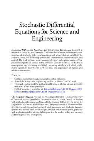


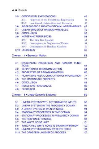
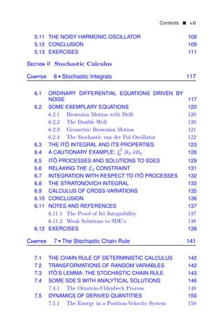


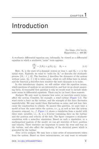
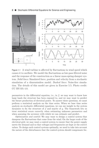
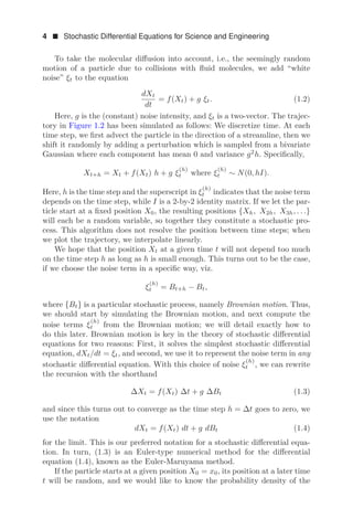
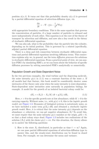
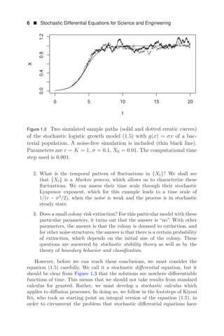
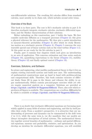


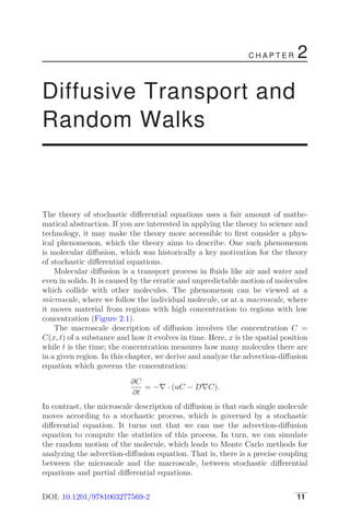
![12 Stochastic Differential Equations for Science and Engineering
Figure 2.1 Diffusion in a container in two dimensions. Top panels: Con-
centration fields. Bottom panels: Position of 100 molecules. Left panels:
Initially, the solute is concentrated at the center. Right panels: After
some time, the solute is less concentrated. The bottom right panel also
includes the trajectory of one molecule; notice its irregular appearance.
2.1 DIFFUSIVE TRANSPORT
In this section, we model how a substance spreads in space due to molecular
diffusion. Think of smoke in still air, or dye in still water. The substance is
distributed over a one-dimensional space R. Let μt([a, b]) denote the amount
of material present in the interval [a, b] at time t. Mathematically, this μt is
a measure. We may measure the substance in terms of number of molecules
or moles, or in terms of mass, but we choose to let μt be dimensionless. We
assume that μt admits a density, which is the concentration C(·, t) of the
substance, so that the amount of material present in any interval [a, b] can be
found as the integral of the concentration over the interval:
μt([a, b]) =
b
a
C(x, t) dx.
The density has unit per length; if the underlying space had been two or three
dimensional, then C would have unit per length squared or cubed, i.e., per
area or per volume. The objective of this section is to pose a partial differential
equation, the diffusion equation (2.3), which governs the time evolution of this
concentration C.](https://image.slidesharecdn.com/24741223-250513084255-5e5cbe2a/85/Stochastic-Differential-Equations-For-Science-And-Engineering-Uffe-Hgsbro-Thygesen-31-320.jpg)
![Diffusive Transport and Random Walks 13
C
x
a b
μ
Ja
Jb
Figure 2.2 Conservation in one dimension. The total mass in the interval
[a, b] is μt([a, b]) =
b
a C(x, t) dx, corresponding to the area of the shaded
region. The net flow into the interval [a, b] is J(a) − J(b).
2.1.1 The Conservation Equation
We first establish the conservation equation
∂C
∂t
+
∂J
∂x
= 0, (2.1)
which expresses that mass is redistributed in space by continuous movements,
but neither created, lost, nor teleported instantaneously between separated
regions in space. To see that this equation holds, note that transport may
then be quantified with a flux J(x, t), which is the net amount of material
that crosses the point x per unit time, from left to right. The flux has physical
dimension “per time”. Then, the amount of material in the interval [a, b] is
only changed by the net influx at the two endpoints, i.e.,
d
dt
μt([a, b]) = J(a, t) − J(b, t).
See Figure 2.2. Assume that the flux J is differentiable in x, then
J(a, t) − J(b, t) = −
b
a
∂J
∂x
(x, t) dx.
On the other hand, since μt is given as an integral, we can use the Leibniz
integral rule to find the rate of change by differentiating under the integral
sign:
d
dt
μt([a, b]) =
b
a
∂C
∂t
(x, t) dx.
Here, we assume that C is smooth so that the Leibniz integral rule applies.
Combining these two expressions for the rate of change of material in [a, b],
we obtain: b
a
∂C
∂t
(x, t) +
∂J
∂x
(x, t)
dx = 0.](https://image.slidesharecdn.com/24741223-250513084255-5e5cbe2a/85/Stochastic-Differential-Equations-For-Science-And-Engineering-Uffe-Hgsbro-Thygesen-32-320.jpg)
![14 Stochastic Differential Equations for Science and Engineering
Since the interval [a, b] is arbitrary, we can conclude that the integrand is
identically 0, or
∂C
∂t
(x, t) +
∂J
∂x
(x, t) = 0.
This is known as the conservation equation. To obtain a more compact nota-
tion, we often omit the arguments (x, t), and we use a dot (as in Ċ) for time
derivative and a prime (as in J
) for spatial derivative. Thus, we can state the
conservation equation compactly as
Ċ + J
= 0.
2.1.2 Fick’s Laws
Fick’s first law for diffusion states that the diffusive flux is proportional to the
concentration gradient:
J(x, t) = −D
∂C
∂x
(x, t) or simply J = −DC
. (2.2)
This means that the diffusion will move matter from regions of high concen-
tration to regions of low concentration. The constant of proportionality, D,
is termed the diffusivity and has dimensions area per time (also when the
underlying space has more than one dimension). The diffusivity depends on
the diffusing substance, the background material it is diffusing in, and the
temperature. See Table 2.1 for examples of diffusivities.
Fick’s first law (2.2) is empirical but consistent with a microscopic model
of molecule motion, as we will soon see. Combining Fick’s first law with the
conservation equation (2.1) gives Fick’s second law, the diffusion equation:
Ċ = (DC
)
. (2.3)
This law predicts, for example, that the concentration will decrease at a peak,
i.e., where C
= 0 and C
0. In many physical situations, the diffusivity D
is constant in space. In this case, we may write Fick’s second law as
Ċ = DC
when D is constant in space, (2.4)
i.e., the rate of increase of concentration is proportional to the spatial curva-
ture of the concentration. However, constant diffusivity is a special situation,
and the general form of the diffusion equation is (2.3).
TABLE 2.1 Examples of Diffusivities
Process Diffusivity [m2
/s]
Smoke particle in air at room temperature 2 × 10⁻⁵
Salt ions in water at room temperature 1 × 10⁻⁹
Carbon atoms in iron at 1250 K 2 × 10−11](https://image.slidesharecdn.com/24741223-250513084255-5e5cbe2a/85/Stochastic-Differential-Equations-For-Science-And-Engineering-Uffe-Hgsbro-Thygesen-33-320.jpg)
![Diffusive Transport and Random Walks 15
Biography: Adolph Eugen Fick (1829–1901)
A German pioneer in biophysics with a background
in mathematics, physics, and medicine. Interested
in transport in muscle tissue, he used the transport
of salt in water as a convenient model system. In
a sequence of papers around 1855, he reported on
experiments as well as a theoretical model of trans-
port, namely Fick’s laws, which were derived as an
analogy to the conduction of heat.
Exercise 2.1: For the situation in Figure 2.2, will the amount of material in
the interval [a, b] increase or decrease in time? Assume that (2.4) applies, i.e.,
the transport is diffusive and the diffusivity D is constant in space.
For the diffusion equation to admit a unique solution, we need an initial
condition C(x, 0) and spatial boundary conditions. Typical boundary condi-
tions either fix the concentration C at the boundary, i.e., Dirichlet conditions,
or the flux J. In the latter case, since the flux J = uC−D∇C involves both the
concentration C and its gradient ∇C, the resulting condition is of Robin type.
In many situations, the domain is unbounded so that the boundary condition
concerns the limit |x| → ∞.
2.1.3 Diffusive Spread of a Point Source
We now turn to an important situation where the diffusion equation admits
a simple solution in closed form: We take the spatial domain to be the entire
real line R, we consider a diffusivity D which is constant in space and time,
and we assume that the fluxes vanish in the limit |x| → ∞. Consider the initial
condition that one unit of material is located at position x0, i.e.,
C(x, 0) = δ(x − x0),
where δ is the Dirac delta. The solution is then a Gaussian bell curve:
C(x, t) =
1
√
2Dt
φ
x − x0
√
2Dt
. (2.5)
Here, φ(·) is the probability density function (p.d.f.) of a standard Gaussian
variable,
φ(x) =
1
√
2π
exp(−
1
2
x2
). (2.6)
Thus, the substance is distributed according to a Gaussian distribution with
mean x0 and standard deviation
√
2Dt; see Figure 2.3. This standard devia-
tion is a characteristic length scale of the concentration field which measures](https://image.slidesharecdn.com/24741223-250513084255-5e5cbe2a/85/Stochastic-Differential-Equations-For-Science-And-Engineering-Uffe-Hgsbro-Thygesen-34-320.jpg)
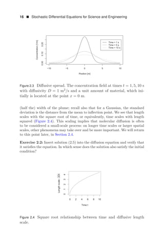
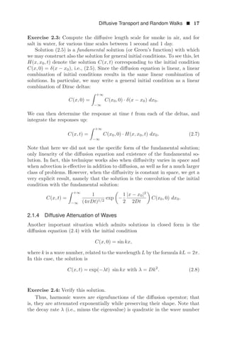
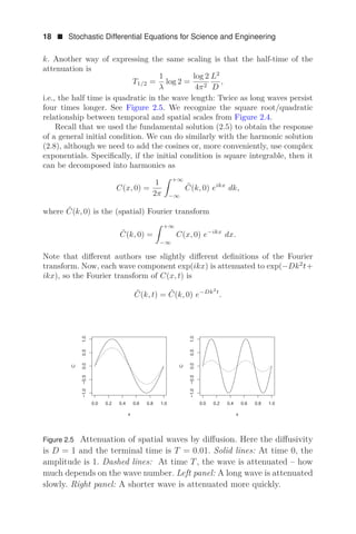
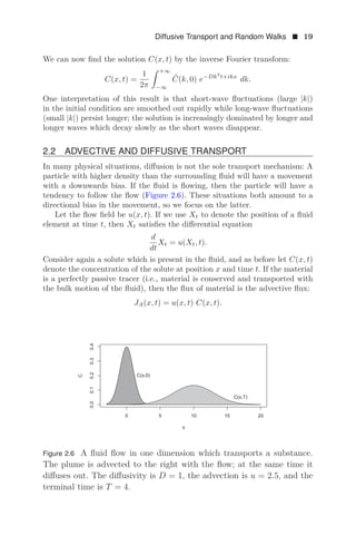
![20 Stochastic Differential Equations for Science and Engineering
If in addition molecular diffusion is in effect, then according to Fick’s first law
(2.2) this gives rise to a diffusive flux JD = −DC
. We may assume that these
two transport mechanisms operate independently, so that the total flux is the
sum of the advective and diffusive fluxes:
J(x, t) = u(x, t) C(x, t) − D(x)
∂C
∂x
(x, t),
or simply J = uC − DC
. Inserting this into the conservation equation (2.1),
we obtain the advection-diffusion equation for the concentration field:
Ċ = −(uC − DC
)
. (2.9)
A simple case is when u and D are constant, the initial condition is a Dirac
delta, C(x, 0) = δ(x − x0), where x0 is a parameter, and the flux vanishes as
|x| → ∞. Then the solution is:
C(x, t) =
1
√
4πDt
exp
−
(x − ut − x0)2
4Dt
, (2.10)
which is the probability density function of a Gaussian random variable with
mean x0 + ut and variance 2Dt. Advection shifts the mean with constant
rate, as if there had been no diffusion, and diffusion gives rise to a linearly
growing variance while preserving the Gaussian shape, as in the case of pure
diffusion (i.e., diffusion without advection). This solution is important, but
also a very special case: In general, when the flow is not constant, it will affect
the variance, and the diffusion will affect the mean.
Exercise 2.5:
1. Verify the solution (2.10).
2. Solve the advection-diffusion equation (2.9) on the real line with con-
stant u and D with the initial condition C(x, 0) = sin(kx) or, if you
prefer, C(x, 0) = exp(ikx).
2.3 DIFFUSION IN MORE THAN ONE DIMENSION
Consider again the one-dimensional situation in Figure 2.2. In n dimensions,
the interval [a, b] is replaced by a region V ⊂ Rn
. Let μt(V ) denote the amount
of the substance present in this region. This measure can be written in terms
of a volume integral of the density C:
μt(V ) =
V
C(x, t) dx.
Here x = (x1, . . . , xn) ∈ Rn
and dx is the volume of an infinitesimal volume
element. The concentration C has physical dimension “per volume”, i.e., SI](https://image.slidesharecdn.com/24741223-250513084255-5e5cbe2a/85/Stochastic-Differential-Equations-For-Science-And-Engineering-Uffe-Hgsbro-Thygesen-39-320.jpg)
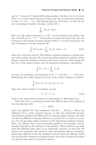
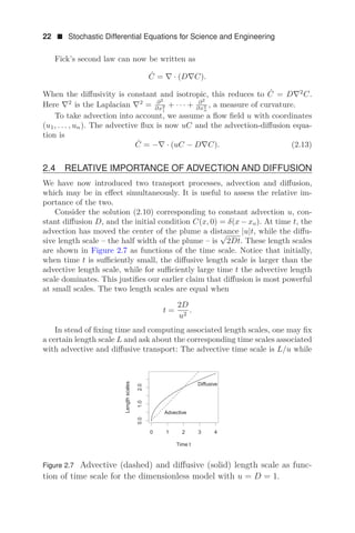
![Diffusive Transport and Random Walks 23
the diffusive time scale is L2
/2D. We define the Péclet number as the ratio
between the two:
Pe = 2
Diffusive time scale
Advective time scale
=
Lu
D
.
It is common to include factor 2 in order to obtain a simpler final expression,
but note that different authors may include different factors. Regardless of the
precise numerical value, a large Péclet number means that the diffusive time
scale is larger than the advective time scale. In this situation, advection is a
more effective transport mechanism than diffusion at the given length scale;
that is, the transport is dominated by advection. Conversely, if the Péclet
number is near 0, diffusion is more effective than advection at the given length
scale. Such considerations may suggest to simplify the model by omitting the
least significant term, and when done cautiously, this can be a good idea.
The analysis in this section has assumed that u and D were constant.
When this is not the case, it is customary to use “typical” values of u and D
to compute the Péclet number. This can be seen as a useful heuristic, but can
also be justified by the non-dimensional versions of the transport equations,
where the Péclet number enters. Of course, exactly which “typical values”
are used for u and D can be a matter of debate, but this debate most often
affects digits and not orders of magnitude. Even the order of magnitude of the
Péclet number is a useful indicator if the transport phenomenon under study
is dominated by diffusion or advection.
Example 2.4.1 Consider the advection-diffusion equation (2.13) in two di-
mensions, where the flow u(x) is around a cylinder. We non-dimensionalize
space so that the cylinder is centered at the origin and has radius 1, and non-
dimensionalize time so that the flow velocity far from the cylinder is 1. Then,
the flow is, in polar coordinates (r, θ) with x = r cos θ, y = r sin θ,
ur(r, θ) = (1 − r−2
) cos θ, uθ = −(1 + r−2
) sin θ.
This is called irrotational flow in fluid mechanics (Batchelor, 1967). A unit of
material is released at time t = 0 at position x = −3, y = −0.5. We solve the
advection-diffusion equation for t ∈ [0, 2.5] for three values of the diffusivity
D: D = 1, D = 0.1, and D = 0.01, leading to the three Péclet numbers 1, 10,
and 100. Figure 2.8 shows the solution at time t = 2.5 for the three Péclet
numbers. Notice how higher Péclet numbers (lower diffusivity D) imply a more
narrow distribution of the material.
2.5 THE MOTION OF A SINGLE MOLECULE
We can accept Fick’s first equation as an empirical fact, but we would like
to connect it to our microscopic understanding. In this section, we present a
caricature of a microscopic mechanism which can explain Fickian diffusion:
Each individual molecule moves in an erratic and unpredictable fashion, due](https://image.slidesharecdn.com/24741223-250513084255-5e5cbe2a/85/Stochastic-Differential-Equations-For-Science-And-Engineering-Uffe-Hgsbro-Thygesen-42-320.jpg)
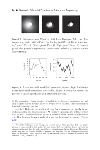
![Diffusive Transport and Random Walks 25
Biography: Robert Brown (1773–1858)
A Scottish botanist who in 1827 studied pollen im-
mersed in water under a microscope and observed
an erratic motion of the grains. Unexplained at
the time, we now attribute the motion to seem-
ingly random collision between the pollen and wa-
ter molecules. The physical phenomenon and its
mathematical model are named Brownian motion,
although many other experimentalists and theoreti-
cians contributed to our modern understanding of
the phenomenon.
In summary, the position {Xt : t ≥ 0} is a random walk:
Xt+h =
⎧
⎨
⎩
Xt + k w.p. (with probability) p,
Xt w.p. 1 − 2p,
Xt − k w.p. p.
.
Here, p ∈ (0, 1
2 ] is a parameter. The displacement in one time step, Xt+h −Xt,
has mean 0 and variance 2k2
p. Displacements over different time steps are
independent, so the central limit theorem applies. After many time steps, the
probability distribution of the displacement Xnh will be well approximated
by a Gaussian with mean 0 and variance 2k2
pn:
Xnh ∼ N(0, 2k2
pn). (2.14)
That is, Xnh will (approximately) have the probability density function
1
2k2pn
· φ(x/ 2k2pn),
where φ is still the p.d.f. of a standard Gaussian variable from (2.6). Next,
assume that we release a large number N of molecules at the origin, and that
they move independently. According to the law of large numbers, the number
of molecules present between x1 and x2 at time nh will be approximately
N
x2
x1
1
2k2pn
· φ(x/ 2k2pn) dx.
Notice that this agrees with equation (2.5), assuming that we take N = 1,
D = k2
p/h and t = nh.
We see that our cartoon model of molecular motion is consistent with the
results of the diffusion equation, if we assume that](https://image.slidesharecdn.com/24741223-250513084255-5e5cbe2a/85/Stochastic-Differential-Equations-For-Science-And-Engineering-Uffe-Hgsbro-Thygesen-44-320.jpg)
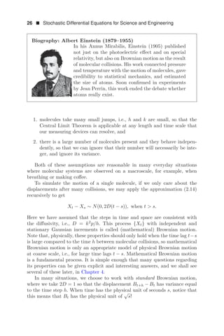
![Diffusive Transport and Random Walks 27
2.6 MONTE CARLO SIMULATION OF PARTICLE MOTION
The previous section considered diffusion only. To add advection, the mi-
croscale picture is that each particle is advected with the fluid while subject
to random collisions with other molecules which randomly perturb the parti-
cle. Thus, each particle performs a biased random walk. When the diffusivity
D and the flow u are constant in space and time, the Gaussian solution (2.10)
to the advection-diffusion equation applies. Then, a random walk model that
is consistent with the advection-diffusion equation is to sample the increments
ΔX = Xt − Xs from a Gaussian distribution
ΔX ∼ N(u · (t − s), 2D(t − s)).
Now what if the flow u = u(x, t) varies in space and time? To simulate the
trajectory of a single particle, it seems to be a reasonable heuristic to divide
the time interval [0, T] into N subintervals
0 = t0, t1, . . . , tN = T.
We first sample X0 from the initial distribution C(·, 0). Then, we sample the
remaining trajectory recursively: At each sub-interval [ti, ti+1], we approxi-
mate the flow field with a constant, namely u(Xti
, ti). This gives us:
Xti+1 ∼ N(Xti + u(Xti ) · Δti, 2D · Δti), (2.15)
where Δti = ti+1 −ti. It seems plausible that, as the time step in this recursion
goes to 0, this approximation becomes more accurate so that the p.d.f. of Xt
will approach the solution C(·, t) to the advection-diffusion equation (2.9).
This turns out to be the case, although we are far from ready to prove it.
Example 2.6.1 (Flow past a cylinder revisited) Example 2.4.1 and Fig-
ure 2.8 present solutions of the advection-diffusion equation for the case where
the flow goes around a cylinder. In the introduction, Figure 1.2 (page 3) show
a trajectory of a single molecule in the same flow. This trajectory is simulated
with the recursion (2.15), using a Péclet number of 200.
The Monte Carlo method, we have just described simulates the motion of
single molecules, chosen randomly from the ensemble. Monte Carlo simulation
can be used to compute properties of the concentration C, but can also answer
questions that are not immediately formulated using partial differential equa-
tions; for example, concerning the time a molecule spends in a region. Monte
Carlo methods are appealing in situations where analytical solutions to the
partial differential equations are not available, and when numerical solutions
are cumbersome, e.g., due to irregular geometries. Monte Carlo methods can
also be useful when other processes than transport are active, for example,
when chemical reactions take place on or between the dispersing particles.](https://image.slidesharecdn.com/24741223-250513084255-5e5cbe2a/85/Stochastic-Differential-Equations-For-Science-And-Engineering-Uffe-Hgsbro-Thygesen-46-320.jpg)
![Diffusive Transport and Random Walks 29
Factbox: [The error function] The physics literature often prefers the “er-
ror function” to the standard Gaussian cumulative distribution function.
The error function is defined as
erf(x) =
2
√
π
x
0
e−s2
ds,
and the complementary error function is
erfc(x) = 1 − erf(x) =
2
√
π
∞
x
e−s2
ds.
These are related to the standard Gaussian distribution function Φ(x) by
erfc(x) = 2 − 2Φ(
√
2x), Φ(x) = 1 −
1
2
erfc(x/
√
2).
erf(x) = 2Φ(
√
2x) − 1, Φ(x) =
1
2
+
1
2
erf(x/
√
2).
2.8 EXERCISES
Exercise 2.6:
1. Solve the diffusion equation (2.4) on the real line with a “Heaviside step”
initial condition
C(x, 0) =
0 when x 0,
1 when x 0.
.
Use boundary conditions limx→+∞ C(x, t) = 1 and limx→−∞ C(x, t) =
0.
Hint: If you cannot guess the solution, use formula (2.7) and manipulate
the integral into a form that resembles the definition of the cumulative
distribution function.
2. Consider the diffusion equation (2.4) on the positive half-line x ≥ 0
with initial condition C(x, 0) = 0 and boundary conditions C(0, t) = 1,
C(∞, t) = 0.
Hint: Utilize the solution of the previous question, and the fact that in
that question, C(0, t) = 1/2 for all t 0.
Exercise 2.7: It is useful to have simple bounds on the tail probabilities in
the Gaussian distribution, such as (Karatzas and Shreve, 1997):
x
1 + x2
φ(x) ≤ 1 − Φ(x) ≤
1
x
φ(x).](https://image.slidesharecdn.com/24741223-250513084255-5e5cbe2a/85/Stochastic-Differential-Equations-For-Science-And-Engineering-Uffe-Hgsbro-Thygesen-48-320.jpg)
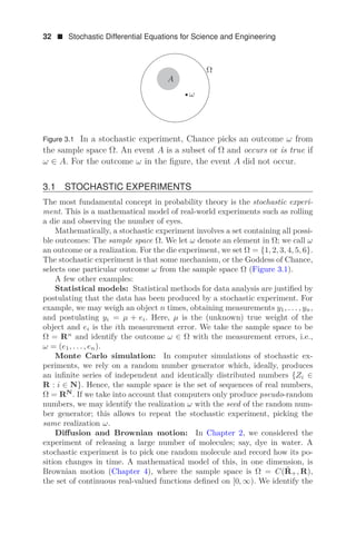
![34 Stochastic Differential Equations for Science and Engineering
to exclude such “non-measurable” subsets of Rn
: They do not correspond to
events.
In elementary probability and statistics, we tend to ignore non-measurable
subsets of Rn
, which have little relevance in applications. However, for more
complicated sample spaces Ω, which appear in the study of stochastic processes
and in particular stochastic differential equations, this difficulty cannot be
ignored: Not all subsets of the sample space can be events, and we often need
careful analysis to determined which ones are.
When not every set A ⊂ Ω can be an event, which ones should be? Some
events are required for the theory to be useful. For example, in the scalar
case Ω = R, we want intervals to correspond to events, so that the statement
ω ∈ [a, b] is an event for any a and b. Moreover, it is imperative that our
machinery of logic works: If A is an event, then the complementary set Ac
must also be an event, so that the statement “not A” is valid. Next, if also
B is an event, then the intersection A ∩ B must also be an event, so that the
statement “A and B” is valid. More generally, in stochastic processes we often
consider infinite sequences of events, for instance when analyzing convergence.
So if {Ai : i ∈ N} is a sequence of events, then the statement “for each integer
i, the statement Ai holds” should be valid. In terms of subsets of sample space
Ω, this means that A1 ∩ A2 ∩ . . . must be an event.
Let F denote the collection of events which we consider. Mathematically
speaking, the requirements on F that we have just argued for, means that F
is a σ-algebra:
Definition 3.1.1 (σ-algebra of events) Given a sample space Ω, a σ-
algebra F of events is a family of subsets of Ω for which:
1. The certain event is included, Ω ∈ F.
2. For each event A ∈ F, the complementary set Ac
is also an event,
Ac
∈ F.
3. Given a sequence of events {Ai ∈ F : i ∈ N}, it is an event that all Ai
occur, i.e., ∩iAi ∈ F.
Given a sequence of events {Ai ∈ F : i ∈ N}, also the union ∪iAi is an event.
Exercise: Verify this!. We often say, for short, that σ-algebras are characterized
by being closed under countable operations of union and intersection.
Example 3.1.1 (The Borel algebra) A specific σ-algebra which we will
encounter frequently in this book, is related to the case Ω = R. We previously
argued that the intervals [a, b] should be events for the theory to be useful in
many situations. The smallest σ-algebra which contains the intervals is called
the Borel-algebra and denoted B(R) or simply B.
The Borel algebra contains all open sets and all closed sets, as well as many
others. This collection of sets is large enough to contain the sets one encoun-
ters in practice, and the fact that the Vitali set and other non-Borel sets exist
is more an excitement to mathematicians than a nuisance to practitioners.](https://image.slidesharecdn.com/24741223-250513084255-5e5cbe2a/85/Stochastic-Differential-Equations-For-Science-And-Engineering-Uffe-Hgsbro-Thygesen-53-320.jpg)
![Stochastic Experiments and Probability Spaces 35
Biography: Félix Édouard Justin Émile Borel (1871–1956)
The French mathematician Borel was one of the
leading figures in the development of measure the-
ory. He applied measure theory to real functions of
real variables, as well as to the foundations of prob-
ability. He was also politically active, argued for a
united Europe, was Minister of the Navy, and was
imprisoned during World War II for assisting the
Resistance.
In the case Ω = Rn
, we require F to include (hyper)rectangles of the form
(a1, b1) × (a2, b2) × . . . × (an, bn), for ai, bi ∈ R and also use the name Borel-
algebra, B(Rn
), for the smallest σ-algebra that contains these hyper-rectangles.
More generally, if Ω is a topological space (i.e., we have defined a system of
open subsets of Ω), then the Borel algebra on Ω is the smallest σ-algebra of
subsets of Ω that contain all the open sets.
It is important to notice that for a given sample space Ω, there can be
several systems of events F. In many applications there is an obvious choice,
but in general, to specify a stochastic experiment, we must state not only
what can happen (i.e., Ω) but also which questions we can ask (i.e., F).
Having outcomes and events in place, we need to assign a probability P(A)
to each event A ∈ F. The way we do this must be consistent:
Definition 3.1.2 (Probability measure) A measure P is a map F →
[0, ∞] which is countably additive, i.e.: P(∪iAi) =
i P(Ai) whenever
A1, A2, . . . are mutually exclusive events (Ai ∩ Aj = ∅ for i = j). A prob-
ability measure is a measure for which P(Ω) = 1.
This definition explains why we call the sets in F measurable: F consists
exactly of those sets, for which the measure P(A) is defined. Notice that
probability is additive only for countable collections of sets, just as the σ-
algebra F must only be closed under countable unions of sets.
An event with probability 0 is called a null event. Conversely, if an event
has probability 1, then we say that this event occurs almost surely (a.s.) or
with probability 1 (w.p. 1).
Example 3.1.2 Consider the uniform distribution on [0, 1); i.e., Ω = [0, 1),
F is the Borel algebra on Ω, and probability corresponds to length, P([a, b]) =
b−a for 0 ≤ a ≤ b 1. Now, the rational numbers form a countable set Q, so
the set A = Ω∩Q is measurable and has measure P(A) = 0: When sampling a
real number uniformly from [0, 1), the probability of getting a rational number
is 0. At the same time, the rationals are dense in [0, 1) (every real number can](https://image.slidesharecdn.com/24741223-250513084255-5e5cbe2a/85/Stochastic-Differential-Equations-For-Science-And-Engineering-Uffe-Hgsbro-Thygesen-54-320.jpg)


![position but the chart of Bering's last voyage, and the exaggerated reports of the
hunters who followed him, must be held responsible for this, in the main.
The work in which this chart appears is largely derived from Müller's Sammlung
russische geschichte, St. Petersburg, 1758, vol. iii, Parts I-III (cf. antea). The first
edition is entitled, according to bibliographies:
Voyages from Asia to America for completing the discoveries of the
northwest coast of America. A summary of voyages made by the
Russians on the frozen sea. From the high Dutch of S[taatsrath]. Muller
by T. Jefferys. London: T. Jefferys, 1761. lxvi, 76 pp. 4°, with four
maps.
The second edition which is that referred to in this paper is entitled
Voyages from Asia to America, for completing the discoveries of the
northwest coast of America. To which is prefixed, a summary of the
Voyages made by the Russians on the Frozen Sea, in search of a
northeast passage. Serving as an explanation of a map of the Russian
discoveries, published by the Academy of Sciences at Petersburgh,
[etc.] London: T. Jefferys, 1764, viii, 120 pp. 4°, four maps.
A French translation by Dumas, with the author's initials misprinted G. P. instead of G. F.,
was printed at Amsterdam in 1766. It consisted of two volumes, 18mo, with a map. A
Danish translation, by Morten Hallager, was issued at Copenhagen in 1784, as a portion
of a volume relating to northern explorations. Bibliographers seem to have been puzzled
by the discrepancy of initials, not recognizing that the S. in Jefferys' volume stood for a
title and not a name. Another work important in its collection of facts bearing upon the
general question of the explorations eastward by the Russians, was published by the
archdeacon of Wilts, Rev. William Coxe in 1780. This was followed by a second edition
during the same year. A third edition accompanied by a Supplement of 57 pages was
printed in 1787 and a fourth in 1803. There were two apparently distinct translations of
the book printed at Paris in 1781, and a German edition at Frankfurt and Leipzig in 1783.
The third edition which is the best and most correct appeared both in octavo and quarto
form, and is that to which reference is made in this paper. It is entitled:
Account of the Russian discoveries between Asia and America. To
which are added the Conquest of Siberia, and the history of the](https://image.slidesharecdn.com/24741223-250513084255-5e5cbe2a/85/Stochastic-Differential-Equations-For-Science-And-Engineering-Uffe-Hgsbro-Thygesen-59-320.jpg)
![transactions and commerce between Russia and China, [etc.]. London:
T. Cadell, 1787.
410 pp. 8° [or 4°] with four charts and one plate; to which is added, consecutively
paged:
A comparative view of the Russian discoveries with those made by
Captains Cook and Clerke, and a sketch of what remains to be
ascertained by future navigators. London: T. Cadell, 1787. 3 l. unp.,
417-456 pp. 8°.
The latter was also separately issued. Among the maps contained in this work of Coxe's
are a reduced copy of the general map of Russia issued by the Imperial Academy of
Sciences, St. Petersburg, 1776, and a chart of Synd's Voyage toward Chukotski Noss.
The latter is the only chart of Synd's voyage (1764-1768) which is accessible, and it is
vouched for as authentic by Dr. Coxe. Compared with later charts it is, of course,
extremely imperfect yet there is in it enough resemblance to the truth to enable us to
recognize what was intended in many instances. In the northeastern part of the chart,
the latitudes are exaggerated and the longitudes contracted in a very erroneous manner.
Nevertheless we recognize East Cape, here named Prom. Tschukotskoi; the two islands
now called the Diomedes but here left nameless; a large island, moved eastward out of
place, but doubtless intended for Arakam Island, is called I. Diomedis; while among a
crowd of islets (referable to the hills of St. Lawrence Island seen through a fog and laid
down very inaccurately), the name S. Diomedis appears again. The American coast
was seen and landed upon; Cape Prince of Wales and the shore south and east from it
are recognizable. The island of St. Mathew was discovered and named, though placed a
degree too far south. The island of St. Paul in the Pribiloff group was discovered by
Synd, put in its true latitude, and named Preobrazhenia or Transfiguration Island. It is
about seven degrees out in relative longitude and fourteen in absolute longitude. One
cannot doubt however that it was the island now known as St. Paul when we recall the
fact that there are no other islands than the Pribiloff group, in that latitude or within that
general area of Bering Sea. The southern Cape of the Chukchi Peninsula, Chukotski Cape
of Bering and Müller is represented two degrees too far south. Preobrazhenia Bay is not
recognizable but the name is transferred to the bight west and north of Cape Bering of
our present charts. This part of the coast was not however approached by Synd, who](https://image.slidesharecdn.com/24741223-250513084255-5e5cbe2a/85/Stochastic-Differential-Equations-For-Science-And-Engineering-Uffe-Hgsbro-Thygesen-60-320.jpg)
![spent much time on the coast of Kamchatka. On his chart this peninsula is represented
better than we should have expected from the rudeness of the rest.
The map of the Academy shows the influence of those who discredited the near
approach of America to eastern Siberia; notwithstanding the explorations of Deshneff,
Gvosdeff and Synd, the American shore of Bering Strait has disappeared altogether. The
eastern portion of the Chukchi Peninsula is indented by a host of hypothetical inlets, and
defended by an unrecognizable archipelago of nameless islands. The far-stretching chain
of islands, among which Bering's second expedition was so long entangled, excepting
those confirmed by Krenitzen and Levasheff (who sailed far north of the southern arc of
the chain) is also absent. Excepting that the fictitious peninsula north from Chukchi land
is effaced, the map in its main features for this region is less accurate than that of
Bering, and does not compare very favorably with that of Müller. And yet but shortly
after its publication, the explorations of Cook and Clerke recorded the facts which
should, when published, exalt the memory of the older geographers and scatter the
hypotheses which for a time prevailed against them.
Their explorations are included in
A voyage to the Pacific Ocean, undertaken by the command of his
Majesty, for making discoveries in the northern hemisphere, [etc.],
performed under the direction of captains Cook, Clerke and Gore, in his
Majesty's ships the Resolution and Discovery, in the years 1776-1780.
London, for T. Nicol and T. Cadell, 1784-5. 3 volumes 4° and atlas
folio.
This is the edition ordered by the Admiralty. Of this celebrated work, said to have been
written from the explorers' manuscripts by Bishop Douglas, there have been many
editions. In the Bulletin of the Société de Géographie, Paris, 1879, pp. 481-540, is a
bibliography by James Jackson.
The most interesting points in regard to Cook's explorations about Bering Strait are
comprised on the chart (vol. ii, p. 467) entitled:
Chart of Norton Sound and of Bherings Strait made by the East Cape
of Asia and the west point of America.](https://image.slidesharecdn.com/24741223-250513084255-5e5cbe2a/85/Stochastic-Differential-Equations-For-Science-And-Engineering-Uffe-Hgsbro-Thygesen-61-320.jpg)
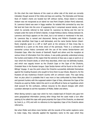
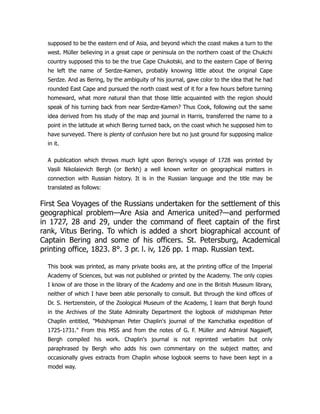
![An effort will be made to obtain a copy of the original logbook,7 but for the present we
are obliged to be content with what of authenticity remains to the data which have been
translated or paraphrased by Bergh, Lauridsen and Olson, necessarily submitting to more
or less modification in the process.
[7 Simultaneously with the proofs of this paper the work of Bergh has been
communicated to me through the liberality of the University of Upsala, Sweden. The
results of a critical examination of it will form the subject of a later paper as the present
publication cannot be delayed.]
The most authentic and important document for the history of this voyage is naturally
the official report handed in by Bering himself and printed in the Journal of the Military
Topographical Depot of the Russian Army, volume x, pp. 67-79, St. Petersburg, 1847.
This journal is a quarto and the report is printed verbatim et literatim if one may judge
by the archaic and mispelled words with which it is adorned. It comprises Bering's report
including his instructions, a table of geographical positions, and a painfully detailed table
of routes and distances by which his position in Kamchatka was computed. This report
has never been translated in full and unmodified, the original is thought to have been
lost. The present publication is not referred to by Lauridsen and was apparently
unknown to him. I have therefore thought it worth while to prepare an English version of
the report and geographical table which are incorporated in this paper.
The result shows that the previous versions of the report which have appeared were
more or less mutilated or colored by the editors printing them, probably with the view of
making the report of more popular interest to their readers but with injurious results to
its historic value for reference.
We now come to the latest contributions to the subject. If it were not for the deficiencies
in them, which seem to me serious, this paper would not have been prepared, but it
seemed to be a pity that the sources of information in regard to Bering, accessible to
those who do not read Russian should not be both more impartial and more accurate.
Vitus J. Bering og de Russiske opdagelsesrejser fra 1725-43. Af P.
Lauridsen. Udgivet med understöttelse af den Hielmstierne-
Rosencroneske stiftelse. Kjöbenhavn. Gyldendalske Boghandels forlag
(F. Hegel Sön). Fr. Bagges bogtrykkeri, 1885. Small 4°, six prel. l.
211 pp., 4 sheets of charts, one plate, one wood-cut.](https://image.slidesharecdn.com/24741223-250513084255-5e5cbe2a/85/Stochastic-Differential-Equations-For-Science-And-Engineering-Uffe-Hgsbro-Thygesen-64-320.jpg)

![modify the criticisms of Bering's character which appear in it; but at the time it was
written I was fresh from four years' exploration in the same region, and was particularly
impressed with his failure to secure better results when to do so would have been so
easy, as well as directly in the line of his duty.]
Review: Bulletin of the American Geographical Society for 1885. New
York, the Society, 1885. pp. 285-298.
This review forms part of a Reply to criticisms upon the voyage of the Vega around Asia
and Europe, by Baron A. E. von Nordenskiold, translated from the Swedish by Vere A.
Elfwing. It is addressed only toward certain points in Lauridsen's work, and contains
valuable corrections of certain errors therein, and information in regard to the work of
Strahlenberg and the other early cartographers of Eastern Siberia. It is a translation of a
paper published in Ymer for 1885, to which for exact accuracy reference should be
made.
Russian explorations, 1725-1743. Vitus Bering: the discoverer of Bering
Strait. By Peter Lauridsen (etc.). Revised by the author and translated
from the Danish by Julius E. Olson (etc.). Chicago, S. C. Griggs
Company, 1889. 8° xvi, 223 pp., 2 cuts, 2 folding sheets of maps.
This edition is a good deal condensed, especially in the matter of references, and does
not have all the illustrations of the original. There are also a good many slips or
typographical errors, which affect its value as a work of reference. Some of those
important in connection with the present paper are as follows: page 31, line 4, 60° 50'
N. latitude should be 62° 50'. On the last line of the same page longitude should be
latitude. Page 32, after cloudy weather in the second line from the bottom, the whole
remaining record of August 15th is omitted altogether. The sentence beginning From
noon relates to August 16th, nautical reckoning. Page 33, line 5, 30° 19' east should
be 30° 17' east; line 20 after half west should be inserted south by east, by
compass. Page 51, line 4 from bottom, latitude should be longitude.
Review: Nation (The) New York, vol. xlix, No. 1275, p. 454. Dec. 5,
1889.
I may add that a number of references to Russian articles treating of
Bering will be found in my Bibliography of charts and publications](https://image.slidesharecdn.com/24741223-250513084255-5e5cbe2a/85/Stochastic-Differential-Equations-For-Science-And-Engineering-Uffe-Hgsbro-Thygesen-66-320.jpg)

![REPORT OF FLEET-CAPTAIN BERING ON HIS EXPEDITION TO THE EASTERN COAST
OF SIBERIA.
To the most Serene Sovereign, the high and powerful, the Empress
of all the Russias:
A short relation of the Siberian Expedition upon which was sent
Of your Imperial Majesty the most humble servant and fleet-captain,
W. I. BERING.
On February 5 of the late year 1725 I received from her Imperial
Majesty the Empress Ekaterina Alexievna, of happy and well-
deserving memory, the autographic instructions of his Imperial
Majesty Peter the Great, of happy and well-deserving memory, a
copy of which is hereunto affixed.
Instructions.
(1.) There should be built on the Kamchatka [River], or at some
other place adjacent, one or two boats with decks.
(2.) With these boats [you are directed] to sail along the coast which
extends northwards and which is supposed (since no one knows the
end of it) to be continuous with America.
(3.) And therefore [you are directed] to seek the point where it
connects with America and to go to some settlement under
European rule, or if any European vessel is seen, learn of it what the
coast visited is called, which should be taken down in writing, an
authentic account prepared, placed on the chart and brought back
here.](https://image.slidesharecdn.com/24741223-250513084255-5e5cbe2a/85/Stochastic-Differential-Equations-For-Science-And-Engineering-Uffe-Hgsbro-Thygesen-68-320.jpg)
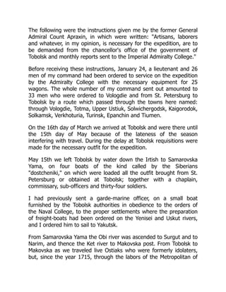
![Tobolsk they have been converted to the true faith. From Makovska
post to Yeniseisk the route lay overland. From Yeniseisk to the Ilima-
mouth we proceeded also in four boats by way of the Yenisei and
Tunguska rivers. On the Tunguska there are three rapids and several
shoals; rapids be it understood where across the whole width of the
river large rocks stand high in the water, with a passage only in one
or two places; and shoals, similarly under water and above water
but composed of small stones, alternate with rapids and with places
where the water in the river is shallow for the distance of one or two
versts, and which are not surmounted without a great deal of labor.
From Yeniseisk in pursuance of orders from Tobolsk we took thirty
men, carpenters and smiths.
On the Ilima river, on account of rapids, bars and shoal water, the
barges could not be taken to Ilimsk. For a certain distance only small
canoes were available, for which reason the heaviest part of the
outfit was reserved to be sent by sledges in winter.
Lieut. Spanberg, with a party of thirty-nine carpenters and laborers,
went by land from Ilimsk by the Uskut to the river Lena, to prepare
during the winter fifteen barges on which the command and its
equipment should be floated down to Yakutsk. I remained with the
rest of the party near Ilimsk just below the Uskut, because at Ilimsk
there are few houses and on account of the difficulties involved in a
winter journey to Yakutsk, from the deficiencies of transportation,
the deep snow and the severe cold, which prevented us from
proceeding.
To these reasons [was added] the necessity, according to the orders
from the authorities at Tobolsk, of drawing the provisions for the
expedition from Irkutsk and from Ilimsk down to Yakutsk because at
the latter place grain is not cultivated. During our wintering at Ilimsk
I made a sledge journey to Irkutsk to advise with the local Voivod
who had previously been Voivod at Yakutsk and who understood
what would be needed by us in transporting our outfit from Yakutsk
to Okhotsk and Kamchatka, since I did not possess any actual](https://image.slidesharecdn.com/24741223-250513084255-5e5cbe2a/85/Stochastic-Differential-Equations-For-Science-And-Engineering-Uffe-Hgsbro-Thygesen-70-320.jpg)
![information in regard to that region. During the last days of winter
travel I went over to the Uskut and obtained from Irkutsk twenty
additional carpenters and smiths for the work of the expedition and
two coopers from Ilimsk.
On the Tunguska, Ilima and Lena rivers to the Vitim live the so-
called Tunguses, people who own reindeer which they use as
draught animals, while those who do not own deer live near the
rivers on fish and travel in canoes made of birch bark. These people
are idolaters.
From Uskutsk on fifteen barges, in the spring of 1726, we descended
the Lena to Yakutsk. From the river Vitim down to the Lena, on both
banks live Yakuts with a smaller proportion of Tunguses. The Yakuts
possess herds of cattle, plenty of horses and cows by which they
subsist, and are contented with the product of their herds,
depending but little on fish except where their cattle are too few.
They pay an idolatrous reverence to the sun and moon as well as to
birds, such as the swan, eagle and crow. They also hold in great
honor their own fortunetellers, known hereabouts as shamani, each
of whom owns small idols or figures which they call shaitan. By their
own account these people are of Tartar origin.
On reaching Yakutsk in boats I required the aid of all the people of
my command. Thirteen flat-bottomed barges which had been
constructed at Uskutsk, under Lieut. Spanberg, proceeded by water
on the Lena down to the Aldan to ascend that river, the Maya and
the upper Yudoma. Such a cargo could hardly have been transported
to that distance overland on horseback where but little in the way of
subsistence was obtainable from land or water. The Cross of Yudoma
might only be reached with great difficulty, but if successful the
expense would be less than if the material had been carried on the
backs of horses. I myself with a few people crossed from Yakutsk to
Okhotsk with pack horses, as is the general custom. The load or
pack taken is only about five puds to one horse, less than by the
telega [ordinary cart], the deep mire and high mountains to be](https://image.slidesharecdn.com/24741223-250513084255-5e5cbe2a/85/Stochastic-Differential-Equations-For-Science-And-Engineering-Uffe-Hgsbro-Thygesen-71-320.jpg)
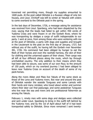
![seven men to Yudoma Cross to bring over the rest of the material on
pack-horses from that place, who returned in May.
In this region in winter time from Yakutsk to Okhotsk and other
distant places people always travel on foot in parties of eight or ten,
hauling their own sledges after them. Those belonging to our
command, when sent from Gorbeh to Okhotsk, brought down ten or
fifteen puds or more, the snow being seven feet deep in places and
travelers in winter being obliged to dig out a camp every evening,
down to the ground to keep warm.
June 30, Lieut. Spanberg in his newly built vessel sailed across the
sea to the port of Bolsheretsk with a cargo of outfit and supplies and
the material for the shipbuilders and workmen of our command, sent
to Kamchatka to get out the timbers for a vessel, being ordered to
return again for us.
July 3d, Lieut. Chirikoff arrived from Yakutsk with 2300 puds of flour,
according to my instructions.
August 21, we loaded the new vessel which had returned from the
land of Kamchatka, and another old boat which had been at
Bolsheretsk, with the flour, and the whole command then at Okhotsk
proceeded across the sea to Bolsheretsk. The officer who had been
left to guard the provisions which had not arrived from the wintering
place on the Gorbeh river was directed to float them down again and
take a receipt from the authorities at Yakutsk and endeavor, the
following year, to deliver to the command in Kamchatka some part of
the provisions, iron and tar.
It was necessary to take the supplies from the mouth of the
[Bolshoia] river to the post of Bolsheretsk by water in small boats. At
the post were fifteen houses inhabited by Russians. For the ascent
of the shallow river small boats had been built as I desired that the
outfit and the most necessary part of the provisions should be
transported to the upper Kamchatka post, a distance of 120 versts](https://image.slidesharecdn.com/24741223-250513084255-5e5cbe2a/85/Stochastic-Differential-Equations-For-Science-And-Engineering-Uffe-Hgsbro-Thygesen-73-320.jpg)
![by water. The transportation between Bolsheretsk and Upper and
Lower Kamchatka in winter was entirely carried on by the use of the
native dogs. Every evening it is necessary to dig out the camp in the
snow, in order to get shelter from whirlwinds of snow which in this
region are called poorga. If one makes camp in an open place free
from snow, these snow squalls are liable to overwhelm the party and
they may perish.
At Upper Kamchatka there are seventeen and at Lower Kamchatka
fifty houses, at another place [Middle Kamchatka] where there is a
church are fifteen houses, and in all these settlements there are not
over 150 Russian subjects, who live by the collection of the yassak
[tribute money], beside those who were brought to the country on
our expedition.
In coming over to Bolsheretsk we brought 300 puds of whale
blubber obtained from a whale cast up by the sea, which served us
as money, together with the Circassian tobacco which is here
commonly so used.
In the southern part of Kamchatka live Kuriles, in the northern part
Kamchadales, whose language is peculiarly their own with but few
introduced words. Of these people some are idolaters, others believe
in nothing and are strangers to all honesty. The Russians who live in
Kamchatka and the indigenes grow no grain and have no domestic
animals except draught dogs. They dress and subsist upon what
they can get, principally fish, roots and berries, in summer time wild
fowl and large marine animals. At present in the wilderness of
Yakutsk, the convent, which is of the same age as the Kamchatka
churches, cultivates barley, hemp and turnips. Here only turnips are
grown by the people of the three settlements, but they grow very
large, in Russia they are smaller, here there may be four turnips to a
pud. I brought with me on my journey some rye which was sowed
around the establishments near us, but whether it ripened or not I
did not ascertain. The frost strikes early into the ground in this](https://image.slidesharecdn.com/24741223-250513084255-5e5cbe2a/85/Stochastic-Differential-Equations-For-Science-And-Engineering-Uffe-Hgsbro-Thygesen-74-320.jpg)
![region and the absence of cattle renders it difficult for the people to
plow.
The natives described and from whom the yassak [tribute] is
collected, belong to the Russian Empire and are all savages. They
are known for their dirt and bad passions. If a woman or any animal
brings forth twins then one of them is smothered, the hour it is
born, and it is regarded as a great fault if one does not smother one
of the two.
The Kamchadales are very superstitious. If there is any one who is
very ill, even a father or mother, or near the point of death, they will
carry them out into the woods and leave them without nourishment
for a week together whether it be winter or summer, from which
treatment many die. The dead are not covered with earth but are
dragged out and left to be eaten by dogs. The house of a man who
has died is abandoned. Among the Kariak people it is the custom to
burn the body, although this is forbidden.
By the time of our arrival at the Lower Kamchatka post the ship-
timber for our vessel was in large part prepared, and upon the 4th of
April, 1728, was put upon the stocks for the vessel, which, with
God's help, was finished by the 10th of July, the timber being hauled
by dogs. Tar was made from the native tree which is called
Listvennik [spruce], since the tar which we should have brought with
us had not arrived.
Before this it was not known here that tar could be obtained from
the native trees. So also for the sea voyage, the deficiency of spirit
made from grain was supplied by a liquor distilled from herbs, and
salt was made by boiling sea water. To increase our store of sea
provisions, in place of cow's butter, fat was tried out from fish, in
place of meat fish was salted. The vessel was provisioned with
everything needful for forty men for a year. On the 14th day of July
we went out of the mouth of the Kamchatka river into the sea, in
obedience to the autographic orders given me by his Imperial](https://image.slidesharecdn.com/24741223-250513084255-5e5cbe2a/85/Stochastic-Differential-Equations-For-Science-And-Engineering-Uffe-Hgsbro-Thygesen-75-320.jpg)