Downloaded 17 times


![Chapter1 Introduction
1
Chapter 1 Introduction
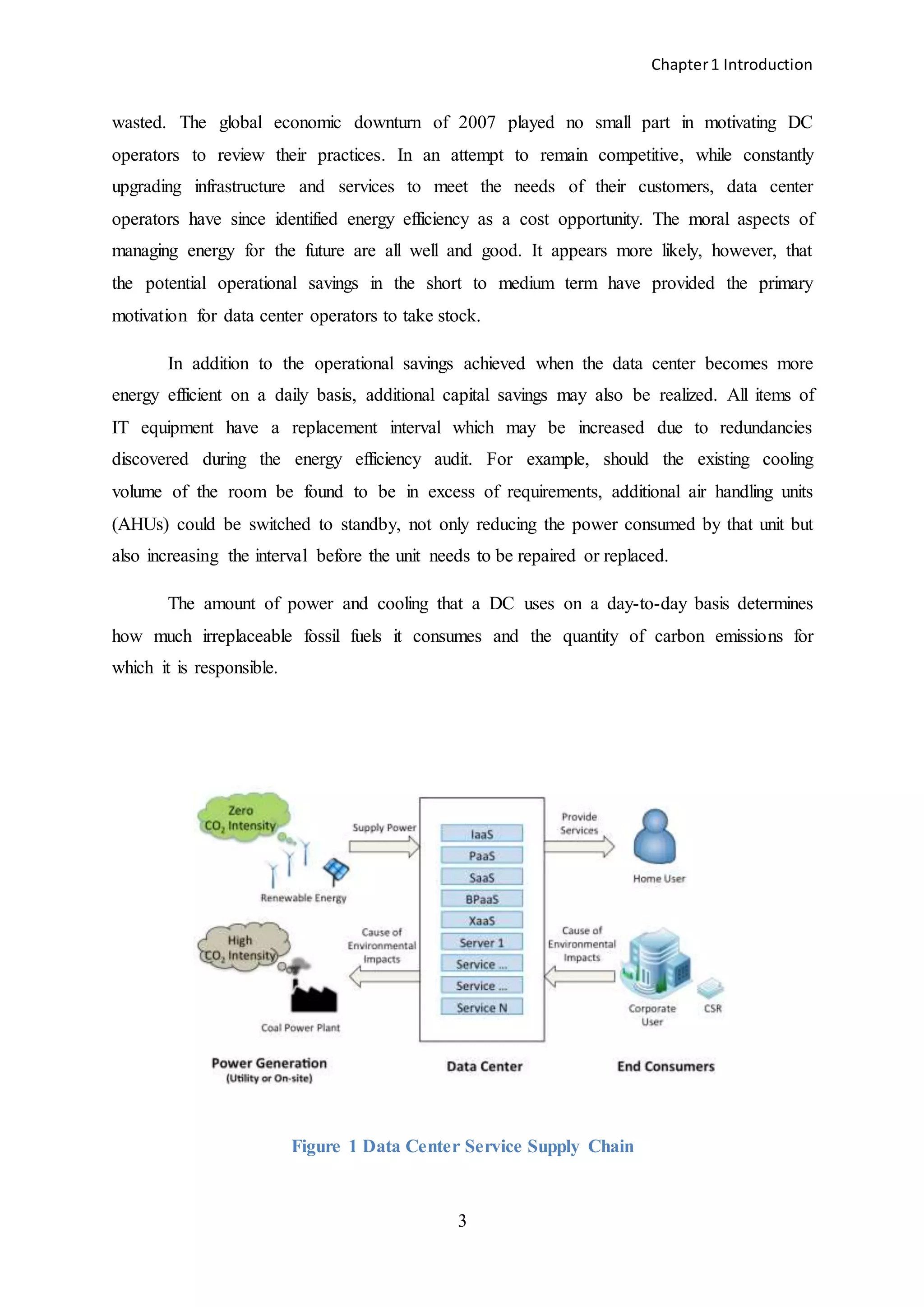
The availability of cloud-based Data Centers (DCs) in recent years has introduced significant
opportunities for enterprises to reduce costs. The initial Capital Expenditure (CapEx)
associated with setting up a DC has been prohibitively high in the past, but this may no
longer be the primary concern. For example, start-ups choosing to implement Infrastructure-
as-a-Service (IaaS) cloud architectures are free to focus on optimizing other aspects of the
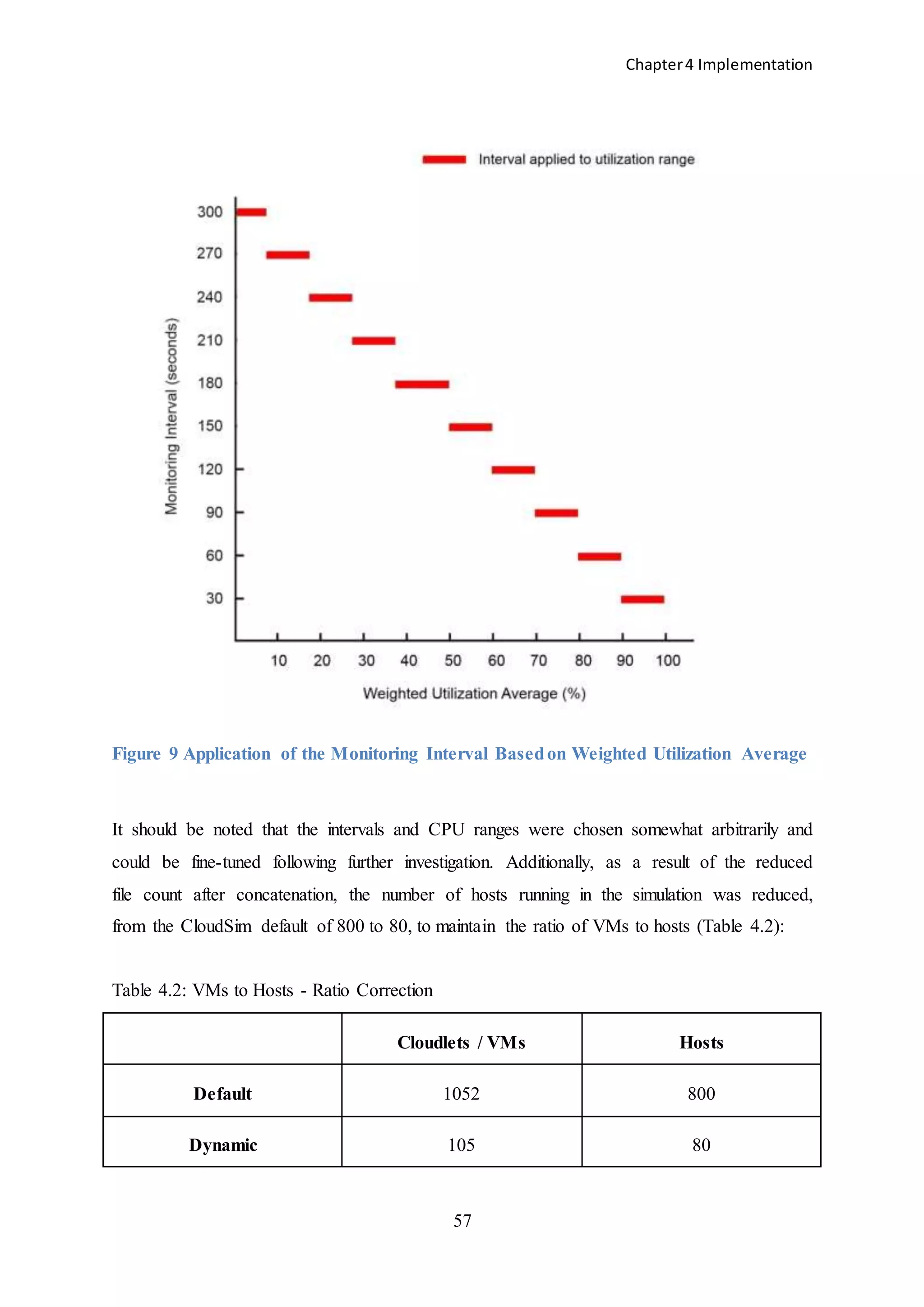
business rather than worrying about raising the capital to build (and maintain) fully equipped
DCs. A young enterprise can now pay a relatively small monthly fee to Amazon (EC2) or
Microsoft (Azure), for example, in return for a scalable infrastructure on which to build their
new product or service. Existing companies are also availing of significant savings and
opportunities by moving to the cloud.
1.1 The Hybrid Cloud
In the future the architecture of cloud computing infrastructure will facilitate a business
moving the public portion of their services from one remote DC to another for cost or
efficiency gains. For example, a DC provider in one US state may be charging less for
compute time because energy costs in that state are lower than those in a neighbouring state.
Migration of enterprise services to the less expensive location could be facilitated. To enable
this type of migratory activity, the Distributed Management Task Force (DMTF) has created
the Open Virtualization Format (OVF) specification. The OVF standard “provides an
intermediary format for Virtual Machine (VM) images. It lets an organization create a VM
instance on top of one hypervisor and then export it to the OVF so that it can be run by
another hypervisor” [4]. With the exception of Amazon, all the major cloud providers (Citrix
Systems, IBM, Microsoft, Oracle and VMware) are involved in the development of OVF.
The short and medium term solution to the interoperability issue will certainly be
‘hybrid’ clouds where the enterprise maintains the private portion of their infrastructure on
their local network and the public portion is hosted on a federated cloud - facilitating indirect
(but not direct) movement between providers e.g. in a similar fashion to switching broadband
providers, a software development company may initially choose to lease a Microsoft data
center for their infrastructure but subsequently transfer to Google if the latter offering](https://image.slidesharecdn.com/f4c2c6b1-e792-48ec-a4d9-218ade73102c-150302055057-conversion-gate01/75/The-Impact-of-Dynamic-Monitoring-Interval-Adjustment-on-Power-Consumption-in-Virtualized-Data-Centers-9-2048.jpg)


![Chapter2 Literature Review
9
In more recent years, increased consumer demand for faster traffic and larger, more flexible,
storage solutions has changed how the industry views the resources required to operate
competitively. More equipment (e.g. servers, routers) has been required to meet demand but
the space required to accommodate this equipment has already been allocated to existing
equipment. The strategy adopted, since 2006, by a DC industry looking to the future, was to
increase the density of IT equipment rather than the more expensive option of purchasing (or
renting) additional square footage. The solution combined new server technologies and
virtualization.
2.2 Increased Density
An analogy: increasing infrastructural density in a data center is similar to adding more
bedrooms to a house without extending the property. The house can now accommodate
private spaces for more people but each person has less space than before. In the data center
there are now more servers per square foot, resulting in more compute / storage capability.
Despite the space-saving advantages of VM technology and techniques (i.e. migration),
which reduced the number of servers required to host applications, the primary disadvantage
of increased density was that each new blade server required significantly more power than
its predecessor. A standard rack with 65-70 blades operating at high loads might require 20 -
30kW of power compared with previous rack consumptions of 2 - 5kW. This additional
power generates additional heat. In a similar manner to maintaining comfortable levels of
heat and humidity for people in a house, heat in the rack, and resultant heat in the server
room, must be removed to maintain the equipment at a safe operating temperature and
humidity. Summarily, the introduction of increased server room density, from 2006 onwards,
resulted in increased power and cooling requirements for modern DCs.
At their 25th Annual Data Center Conference held in Las Vegas in late November
2006, Gartner analysts hypothesized that:
“…by 2008, 50% of current data centers will have insufficient
power and cooling capacity to meet the demands of high-density
equipment…” [1]](https://image.slidesharecdn.com/f4c2c6b1-e792-48ec-a4d9-218ade73102c-150302055057-conversion-gate01/75/The-Impact-of-Dynamic-Monitoring-Interval-Adjustment-on-Power-Consumption-in-Virtualized-Data-Centers-17-2048.jpg)
![Chapter2 Literature Review
10
During his address to the conference, Gartner Research Vice President, Michael Bell
suggested that: “Although power and cooling challenges will not be a perpetual problem, it is
important for DC managers to focus on the electrical and cooling issue in the near term, and
adopt best practice to mitigate the problem before it results in equipment failure, downtime
and high remediation costs”. This was one of the first ‘shots across the bow’ for a data center
industry which, until then, had been solely focussed on improving performance (e.g. uptime,
response time) almost in deference to escalating energy costs.
Based on data provided by IDC [2], Jonathon Koomey published a report [3] in
February 2007 estimating the electricity used by all DCs in both the US and globally for
2005. The executive summary states that:
“The total power demand in 2005 (including associated
infrastructure) is equivalent (in capacity terms) to about five 1000
MW power plants for the U.S. and 14 such plants for the world. The
total electricity bill for operating those servers and associated
infrastructure in 2005 was about $2.7 billion and $7.2 billion for the
U.S. and the world, respectively.”
A few months later the global economic downturn brought with it increasingly restrictive
operating budgets and higher energy prices. The competitive edge was becoming harder to
identify. Quite apart from the economic factors affecting the industry, the timely publication
by the EPA of its report to the US Congress [4] in August 2007 highlighted significant
opportunities to reduce both capital and operating costs by optimizing the power and cooling
infrastructure involved in data center operations. Industry analysts were once again
identifying an escalating power consumption trend which required immediate attention.
The report assessed the principle opportunities for energy efficiency improvements in
US DCs. The process of preparing the report brought all the major industry players together.
In an effort to identify a range of energy efficiency opportunities, 3 main improvement
scenarios were formulated:
1. Improved Operation: maximizes the efficiency of the existing data center
infrastructure by utilizing improvements such as ‘free cooling’ and raising](https://image.slidesharecdn.com/f4c2c6b1-e792-48ec-a4d9-218ade73102c-150302055057-conversion-gate01/75/The-Impact-of-Dynamic-Monitoring-Interval-Adjustment-on-Power-Consumption-in-Virtualized-Data-Centers-18-2048.jpg)
![Chapter2 Literature Review
12
2.3 Hardware
Rasmussen [5] identified power distribution, conversion losses and cooling as representing
between 30 – 45% of the electricity bill in larger DCs. Cooling alone accounted for 30% of
this total.
Figure 2 Relative contributions to the thermal output of a typical DC
2.3.1 Uninterruptible Power Supply (UPS) & Power Distribution
The power being provided to the IT equipment in the racks is typically routed through an
Uninterruptible Power Supply (UPS) which feeds Power Distribution Units (PDUs) located
in or near the rack. Through use of better components, circuit design and right-sizing
strategies, manufacturers such as American Power Conversion (APC) and Liebert have
turned their attention to maximizing efficiency across the full load spectrum, without](https://image.slidesharecdn.com/f4c2c6b1-e792-48ec-a4d9-218ade73102c-150302055057-conversion-gate01/75/The-Impact-of-Dynamic-Monitoring-Interval-Adjustment-on-Power-Consumption-in-Virtualized-Data-Centers-20-2048.jpg)
![Chapter2 Literature Review
14
Figure 3 A Typical AHU Direct Expansion (DX) Cooling System
Depending on the configuration, the heat removal system might potentially consume 50% of
a typical DC’s energy. Industry is currently embracing a number of opportunities involving
temperature and airflow analysis:
1. aisle containment strategies
2. increasing the temperature rise (ΔT) across the rack
3. raising the operating temperature of the AHU(s)
4. repositioning AHU temperature and humidity sensors
5. thermal management by balancing the IT load layout [6, 7]
6. ‘free cooling’ – eliminating the high-consumption chiller from the system through
the use of strategies such as air- and water-side economizers](https://image.slidesharecdn.com/f4c2c6b1-e792-48ec-a4d9-218ade73102c-150302055057-conversion-gate01/75/The-Impact-of-Dynamic-Monitoring-Interval-Adjustment-on-Power-Consumption-in-Virtualized-Data-Centers-22-2048.jpg)
![Chapter2 Literature Review
15
Figure 4 A Typical DC Air Flow System
In addition to temperature maintenance, the AHUs also vary the humidity of the air entering
the server room according to set-points. Low humidity (dry air) may cause static which has
the potential to short electronic circuits. High levels of moisture in the air may lead to faster
component degradation. Although less of a concern as a result of field experience and recent
studies performed by Intel and others, humidity ranges have been defined for the industry and
should be observed to maximize the lifetime of the IT equipment. Maintaining humidity
ranges definitively increases the interval between equipment replacement schedules and, as a
result, has a net positive outcome on capital expenditure budgets.
2.3.4 Industry Standards & Guidelines
2.3.4.1 Standards
Power Usage Effectiveness (PUE2) [8] is now the de facto standard used to measure a DC’s
efficiency. It is defined as the ratio of all electricity used by the DC to the electricity used just
by the IT equipment. In contrast to the original PUE [9] rated in kilowatts of power (kW),
PUE2 must be based on the highest measured kilowatt hour (kWh) reading taken during
analysis. In 3 of the 4 PUE2 categories now defined, the readings must span a 12 month
period, eliminating the effect of seasonal fluctuations in ambient temperatures:
PUE =
𝑇𝑜𝑡𝑎𝑙 𝐷𝑎𝑡𝑎 𝐶𝑒𝑛𝑡𝑟𝑒 𝐸𝑙𝑒𝑐𝑡𝑟𝑖𝑐𝑖𝑡𝑦 ( 𝑘𝑊ℎ)
𝐼𝑇 𝐸𝑞𝑢𝑖𝑝𝑚𝑒𝑛𝑡 𝐸𝑙𝑒𝑐𝑡𝑟𝑖𝑐𝑖𝑡𝑦 ( 𝑘𝑊ℎ)](https://image.slidesharecdn.com/f4c2c6b1-e792-48ec-a4d9-218ade73102c-150302055057-conversion-gate01/75/The-Impact-of-Dynamic-Monitoring-Interval-Adjustment-on-Power-Consumption-in-Virtualized-Data-Centers-23-2048.jpg)
![Chapter2 Literature Review
16
A PUE of 2.0 suggests that for each kWh of IT electricity used another kWh is used by the
infrastructure to supply and support it. The most recent PUE averages [10] for the industry
fall within the range of 1.83 – 1.92 with worst performers coming in at 3.6 and a few top
performers publishing results below 1.1 in recent months. Theoretically, the best possible
PUE is 1.0 but a web-hosting company (Pair Networks) recently quoted a PUE of 0.98 for
one of its DCs in Las Vegas, Nevada. Their calculation was based on receipt of PUE ‘credit’
for contributing unused power (generated on-site) back to the grid. Whether additional PUE
‘credit’ should be allowed for contributing to the electricity grid is debatable. If this were the
case, with sufficient on-site generation, PUE could potentially reach 0.0 and cease to have
meaning. Most DCs are now evaluating their own PUE ratio to identify possible
improvements in their power usage. Lower PUE ratios have become a very marketable aspect
of the data center business and have been recognized as such. Other standards and metrics
(2.3.4.2.1 – 2.3.4.2.4) have been designed for the industry but, due for the most part to the
complex processes required to calculate them, have not as yet experienced the same wide-
spread popularity as PUE and PUE2.
2.3.4.2 Other Standards
2.3.4.2.1 Water Usage Effectiveness (WUE) measures DC water usage to provide an
assessment of the water used on-site for operation of the data center. This includes water used
for humidification and water evaporated on-site for energy production or cooling of the DC
and its support system.
2.3.4.2.2 Carbon Usage Effectiveness (CUE) measures DC-level carbon emissions.
CUE does not cover the emissions associated with the lifecycle of the equipment in the DC or
the building itself.
2.3.4.2.3 The Data Center Productivity (DCP) framework is a collection of metrics
which measure the consumption of a DC-related resource in terms of DC output. DCP looks
to define what a data center accomplishes relative to what it consumes.
2.3.4.2.4 Data Center Compute Efficiency (DCCE) enables data center operators to
determine the efficiency of compute resources. The metric makes it easier for data center
operators to discover unused servers (both physical and virtual) and decommission or
redeploy them.](https://image.slidesharecdn.com/f4c2c6b1-e792-48ec-a4d9-218ade73102c-150302055057-conversion-gate01/75/The-Impact-of-Dynamic-Monitoring-Interval-Adjustment-on-Power-Consumption-in-Virtualized-Data-Centers-24-2048.jpg)
![Chapter2 Literature Review
17
Surprisingly, efforts to improve efficiency have not been implemented to the extent one
would expect. 73% of respondents to a recent Uptime Institute survey [11] stated that
someone outside of the data center (the real estate / facilities department) was responsible for
paying the utility bill. 8% of data center managers weren’t even aware who paid the bill. The
lack of accountability is obvious and problematic. If managers are primarily concerned with
maintaining the DC on a daily basis there is an inevitable lack of incentive to implement even
the most basic energy efficiency strategy in the short to medium term. It is clear that a
paradigm shift is required to advance the cause of energy efficiency monitoring at the ‘C-
level’ (CEO, CFO, CIO) of data center operations.
2.3.4.3 Guidelines
Data center guidelines are intermittently published by The American Society of Heating,
Refrigeration and Air Conditioning Engineers (ASHRAE). These guidelines [12, 13] suggest
‘allowable’ and ‘recommended’ temperature and humidity ranges within which it is safe to
operate IT equipment. The most recent edition of the guidelines [14] suggests operating
temperatures of 18 – 27⁰C. The maximum for humidity is 60% RH.
One of the more interesting objectives of the recent guidelines is to have the rack inlet
recognized as the position from where the temperature and humidity should be measured. The
majority of DCs currently measure at the return inlet to the AHU, despite more relevant
temperature and humidity metrics being present at the inlet to the racks.
2.3.5 Three Seminal Papers
In the context of improving the hardware infrastructure of the DC post-2006, three academic
papers were found to be repeatedly referenced as forming a basis for the work of the most
prominent researchers in the field. They each undertake a similar methodology when
identifying solutions and are considered to have led the way for a significant number of
subsequent research efforts. The methodologies which are common to each of the papers (and
relevant to this thesis) include:
1. Identification of a power consumption opportunity within the DC and adoption of
a software-based solution](https://image.slidesharecdn.com/f4c2c6b1-e792-48ec-a4d9-218ade73102c-150302055057-conversion-gate01/75/The-Impact-of-Dynamic-Monitoring-Interval-Adjustment-on-Power-Consumption-in-Virtualized-Data-Centers-25-2048.jpg)
![Chapter2 Literature Review
18
2. Demonstration of the absolute requirement for monitoring the DC environment as
accurately as possible without overloading the system with additional processing
Summary review of the three papers follows.
2.3.5.1 Paper 1: Viability of Dynamic Cooling Control in a Data Center
Environment (2006)
In the context of dynamically controlling the cooling system Boucher et al. [15] focused their
efforts on 3 requirements:
1. A distributed sensor network to indicate the local conditions of the data center.
Solution: a network of temperature sensors was installed at:
Rack inlets
Rack outlets
Tile inlets
2. The ability to vary cooling resources locally. Solution: 4 actuation points, which exist
in a typical data center, were identified as having further potential in maintaining
optimal server room conditions:
2.1 CRAC supply temperature – this is the temperature of the conditioned air
entering the room. CRACs are typically operated on the basis of a single
temperature sensor at the return side of the unit. This sensor is responsible for
taking an average of the air temperature returning from the room. The CRAC then
correlates this reading with a set-point which is configured manually by data
center staff. The result of the correlation is the basis upon which the CRAC
decides by how much the temperature of the air sent back out into the room should
be adjusted. Variation is achieved in a Direct Expansion (DX) system with
variable capacity compressors varying the flow of refrigerant across the cooling
coil. In a water-cooled system chilled water supply valves modulate the
temperature.
2.2 The crucial element in the operational equation of the CRAC, regardless of the
system deployed, is the set-point. The set-point is manually set by data center staff
and generally requires considerable analysis of the DC environment before any](https://image.slidesharecdn.com/f4c2c6b1-e792-48ec-a4d9-218ade73102c-150302055057-conversion-gate01/75/The-Impact-of-Dynamic-Monitoring-Interval-Adjustment-on-Power-Consumption-in-Virtualized-Data-Centers-26-2048.jpg)
![Chapter2 Literature Review
20
continuous maximum efficiency. Boucher et al. propose that this control system
should be based on the 4 available actuation points above.
3. The knowledge of each variable’s effect on DC environment. Solution: the paper
focused on how each of the actuator variables (2.1, 2.2 and 2.3 and 2.4 above) can
affect the thermal dynamic of the data center.
Included in the findings of the study were:
CRAC supply temperatures have an approximate linear relationship with rack inlet
temperatures. An anomaly was identified where the magnitude of the rack inlet
response to a change in CRAC supply temperature was not of the same order. Further
study was suggested.
Under-provisioned flow provided by the CRAC fans affects the Supply Heat Index
(SHI*) but overprovisioning has a negligible effect. SHI is a non-dimensional
measure of the local magnitude of hot and cold air mixing. Slower air flow rates cause
an increase in SHI (more mixing) whereas faster air flow rates have little or no effect.
*SHI is also referred to as Heat Density Factor (HDF). The metric is based on the
principle of a thermal multiplier which was formulated by Sharma et al. [16]
The study concluded that significant energy savings (in the order of 70% in this case) were
possible where a dynamic cooling control system, controlled by software, was appropriately
deployed.
2.3.5.2 Paper 2: Impact of Rack-level Compaction on the Data Center Cooling
Ensemble (2008)
Shah et al. [17] deal with the impact on the data center cooling ensemble when the density of
compute power is increased. The cooling ‘ensemble’ is considered to be all elements of the
cooling system from the chip to the cooling tower.
Increasing density involves replacing low-density racks with high-density blade
servers and has been the chosen alternative to purchasing (or renting) additional space for](https://image.slidesharecdn.com/f4c2c6b1-e792-48ec-a4d9-218ade73102c-150302055057-conversion-gate01/75/The-Impact-of-Dynamic-Monitoring-Interval-Adjustment-on-Power-Consumption-in-Virtualized-Data-Centers-28-2048.jpg)
![Chapter2 Literature Review
21
most DCs in recent years. New enterprise and co-location data centers also implement the
strategy to maximize the available space. Densification leads to increased power dissipation
and corresponding heat flux within the DC environment.
A typical cooling system performs two types of work:
1. Thermodynamic – removes the heat dissipated by the IT equipment
2. Airflow – moves the air through the data center and related systems
The metric chosen by Shah et al. for evaluation in this case is the ‘grand’ Coefficient of
Performance (COPG) which is a development of the original COP metric suggested by Patel
et al. [18, 19]. It measures the amount of heat removed by the cooling infrastructure per unit
of power input and does so at a more granular level than the traditional COP used in
thermodynamics, specifying heat removal at the chip, system, rack, room and facility levels.
In order to calculate the COPG of the model used for the test case each component of
the cooling system needed to be evaluated separately, before applying each result to the
overall system. Difficulties arose where system-level data was either simply unavailable or,
due to high heterogeneity, impossible to infer. However, the model was generic enough that it
could be applied to the variety of cooling systems currently being used by ‘real world’ DCs.
Note: in a similar vein, the research for this thesis examines the CPU utilization of
each individual server in the data center such that an overall DC utilization metric at each
interval can be calculated. Servers which are powered-off at the time of monitoring have no
effect on the result and are excluded from the calculation.
The assumption that increased density leads to less efficiency in the cooling system is
incorrect. If elements of the cooling system were previously running at low loads they would
typically have been operating at sub-optimal efficiency levels. Increasing the load on a
cooling system may in fact increase its overall efficiency through improved operational
efficiencies in one or more of its subsystems.
94 existing low-density racks were replaced with high-density Hewlett Packard (HP) blades
for Shah’s research. The heat load increased from 1.9MW to 4.7MW. The new heat load was
still within the acceptable range for the existing cooling infrastructure. No modifications to
the ensemble were required.](https://image.slidesharecdn.com/f4c2c6b1-e792-48ec-a4d9-218ade73102c-150302055057-conversion-gate01/75/The-Impact-of-Dynamic-Monitoring-Interval-Adjustment-on-Power-Consumption-in-Virtualized-Data-Centers-29-2048.jpg)
![Chapter2 Literature Review
22
Upon analysis of the results, COPG was found to have increased by 15%. This was, in part,
achieved with improved efficiencies in the compressor system of the CRACs. While it is
acknowledged that there is a crossover point at which compressors become less efficient, the
increase in heat flux of the test model resulted in raising the work of the compressor to a
point somewhere below this crossover. The improvement in compressor efficiency was
attributed to the higher density HP blade servers operating at a higher ΔT (reduced flow rates)
across the rack. The burden on the cooling ensemble was reduced - resulting in a higher
COPG.
With the largest individual source of DC power consumption (about 40% in this case)
typically coming from the CRAC - which contains the compressor - it makes sense to direct
an intelligent analysis of potential operational efficiencies at that particular part of the system.
The paper states that: “The continuously changing nature of the heat load distribution
in the room makes optimization of the layout challenging; therefore, to compensate for
recirculation effects, the CRAC units may be required to operate at higher speeds and lower
supply temperature than necessary. Utilization of a dynamically coupled thermal solution,
which modulates the CRAC operating points based on sensed heat load, can help reduce this
load”.
In this paper Shah et al. present a model for performing evaluation of the cooling
ensemble using COPG, filling the gap of knowledge through detailed experimentation with
measurements across the entire system. They conclude that energy efficiencies are possible
via increased COP in one or more of the cooling infrastructure components. Where thermal
management strategies capable of handling increased density are in place, there is significant
motivation to increase density without any adverse impact on energy efficiency.
2.3.5.3 Paper 3: Data Center Efficiency with Higher Ambient Temperatures and
Optimized Cooling Control (2011)
Ahuja et al. [20] introduce the concept of ‘deviation from design intent’. When a data center
is first outfitted with a cooling system, best estimates are calculated for future use. The
intended use of the DC in the future is almost impossible to predict at this stage. As the
lifecycle of the DC matures, the IT equipment will deviate from the best estimates upon](https://image.slidesharecdn.com/f4c2c6b1-e792-48ec-a4d9-218ade73102c-150302055057-conversion-gate01/75/The-Impact-of-Dynamic-Monitoring-Interval-Adjustment-on-Power-Consumption-in-Virtualized-Data-Centers-30-2048.jpg)
![Chapter2 Literature Review
23
which the cooling system was originally designed to operate. Without on-going analysis of
the DC’s thermal dynamics, the cooling system may become decreasingly ‘fit-for-purpose’.
As a possible solution to this deviation from intent, this paper proposes that cooling of
the DC environment should be controlled from the chip rather than a set of remote sensors in
the room or on the rack doors. Each new IT component would have chip-based sensing
already installed and therefore facilitate a “plug ‘n’ play” cooling system.
The newest Intel processors (since Intel® Pentium® M) on the market feature an ‘on-
die’ Digital Thermal Sensor (DTS). DTS provides the temperature of the processor and
makes the result available for reading via Model Specific Registers (MSRs). The Intel white
paper [21] which describes DTS states that:
“… applications that are more concerned about power consumption
can use thermal information to implement intelligent power
management schemes to reduce consumption.”
While Intel is referring to power management of the server itself, DTS could
theoretically be extended to the cooling management system also.
Current DCs control the air temperature and flow rate from the chip to the chassis but
there is a lack of integration once the air has left the chassis. If the purpose of the data center
is to house, power and cool every chip then it has the same goal as the chassis and the chassis
is already taking its control data from the chip. This strategy needs to be extended to the
wider server room environment in an integrated manner.
The industry has recently been experimenting with positioning the cooling sensors at
the front of the rack rather than at the return inlet of the AHU. The motivation for this is to
sense the air temperature which matters most – the air which the IT equipment uses for
cooling. The disadvantage of these remote sensors (despite being better placed than sensors at
the AHU return inlet) is that they are statically positioned, a position which may later be
incorrect should changes in the thermal dynamics of the environment occur. The closer to the
server one senses - the more reliable the sensed data will be for thermal control purposes.
Ahuja et al. propose that the logical conclusion is to move the sensors even closer to the](https://image.slidesharecdn.com/f4c2c6b1-e792-48ec-a4d9-218ade73102c-150302055057-conversion-gate01/75/The-Impact-of-Dynamic-Monitoring-Interval-Adjustment-on-Power-Consumption-in-Virtualized-Data-Centers-31-2048.jpg)
![Chapter2 Literature Review
25
on this 'over-utilized' host to a similar VM on another physical server, where sufficient
capacity (e.g. CPU) is available to maintain SLA performance.
Conversely, reduced demand on the CPU of a host introduces opportunities for server
consolidation, the objective of which is to minimize the number of operational servers
consuming power. The remaining VMs on an 'under-utilized' host are migrated so that the
host can be switched off, saving power. Server consolidation provides significant energy
efficiency opportunities.
There are numerous resource allocation schemes for managing VMs in a data center,
all of which involve the migration of a VM from one host to another to achieve one, or a
combination of, objectives. Primarily these objectives will involve either increased
performance or reduced energy consumption - the former, until recently, receiving more of
the operator’s time and effort than the latter.
In particular, SLA@SOI has completed extensive research in recent years in the area
of SLA-focused (e.g. CPU, memory, location, isolation, hardware redundancy level) VM
allocation and re-provisioning [22]. The underlying concept is that VMs are assigned to the
most appropriate hosts in the DC according to both service level and power consumption
objectives. Interestingly, Hyser et al. [23] suggest that a provisioning scheme which also
includes energy constraints may choose to violate user-based SLAs ‘if the financial penalty
for doing so was [sic] less than the cost of the power required to meet the agreement’. In a
cost-driven DC it is clear that some trade-off (between meeting energy objectives and
compliance with strict user-based SLAs e.g. application response times) is required. A similar
power / performance trade-off may be required to maximize the energy efficiency of a host-
level migration.
2.4.2 Migration
The principal underlying technology which facilitates management of workload in a DC is
virtualization. Rather than each server hosting a single operating system (or application),
virtualization facilitates a number of VMs being hosted on a single physical server, each of
which may run a different operating system (or even different versions of the same operating](https://image.slidesharecdn.com/f4c2c6b1-e792-48ec-a4d9-218ade73102c-150302055057-conversion-gate01/75/The-Impact-of-Dynamic-Monitoring-Interval-Adjustment-on-Power-Consumption-in-Virtualized-Data-Centers-33-2048.jpg)
![Chapter2 Literature Review
26
system). These VMs may be re-located (migrated) to a different host on the LAN for a
variety of reasons:
Maintenance
Servers intermittently need to be removed from the network for maintenance. The
applications running on these servers may need to be kept running during the
maintenance period so they are migrated to other servers for the duration.
Consolidation
In a virtualized DC some of the servers may be running at (or close to) idle – using
expensive power to maintain a machine which is effectively not being used to
capacity. To conserve power, resource allocation software moves the applications on
the under-utilized machine to a ‘busier’ machine - as long as the latter has the
required overhead to host the applications. The under-utilized machine can then be
switched off – saving on power and cooling.
Energy Efficiency
Hotspots regularly occur in the server room i.e. the cooling system is working too
hard in the effort to eliminate the exhaust air from a certain area. The particular
workload which is causing the problem can be identified and relocated to a cooler
region in the DC to relieve the pressure in the overheated area.
Virtual Machines may also be migrated to servers beyond the LAN (i.e. across the Wide Area
Network (WAN):
Follow the sun - minimize network latency during office hours by placing VMs close
to where their applications are requested most often
Where latency is not a primary concern there are a number of different strategies
which may apply:
Availability of renewable energy / improved energy mix
Less expensive cooling overhead (e.g. ‘free’ cooling in more temperate / cooler
climates
Follow the moon (less expensive electricity at night)
Fluctuating electricity prices on the open market [24]](https://image.slidesharecdn.com/f4c2c6b1-e792-48ec-a4d9-218ade73102c-150302055057-conversion-gate01/75/The-Impact-of-Dynamic-Monitoring-Interval-Adjustment-on-Power-Consumption-in-Virtualized-Data-Centers-34-2048.jpg)
![Chapter2 Literature Review
27
Disaster Recovery (DR)
Maintenance / Fault tolerance
Bursting i.e. temporary provisioning of additional resources
Backup / Mirroring
Regardless of the motivation, migration of virtual machines both within the DC and also to
other DCs (in the cloud or within the enterprise network) not only extends the opportunity for
significant cost savings but may also provide faster application response times if located
closer to clients. To maintain uptime and response Service Level Agreement (SLAs)
parameters of 99.999% (or higher), these migrations must be performed ‘hot’ or ‘live’,
keeping the application available to users while the virtual machine hosting the application
(and associated data) is moved to the destination server. Once all the data has been migrated,
requests coming into the source VM are redirected to the new machine and the source VM
can be switched off or re-allocated. The most popular algorithm by which virtual machines
are migrated is known as pre-copy and is deployed by both Citrix and VMWare – currently
considered to be the global leaders in software solutions for migration and virtualized
systems. A variety of live migration algorithms have been developed in the years since 2007.
Some are listed below:
1. Pre-copy [25]
2. GA for Renewable Energy Placement [26]
3. pMapper: Power Aware Migration [27]
4. De-duplication, Smart Stop & Copy, Page Deltas & CBR (Content Based
Replication) [28]
5. Layer 3: IP LightPath [29]
6. Adaptive Memory Compression [30]
7. Parallel Data Compression [31]
8. Adaptive Pre-paging and Dynamic Self-ballooning [32]
9. Replication and Scheduling [33]](https://image.slidesharecdn.com/f4c2c6b1-e792-48ec-a4d9-218ade73102c-150302055057-conversion-gate01/75/The-Impact-of-Dynamic-Monitoring-Interval-Adjustment-on-Power-Consumption-in-Virtualized-Data-Centers-35-2048.jpg)
![Chapter2 Literature Review
28
10. Reinforcement Learning [34]
11. Trace & Replay [35]
12. Distributed Replicated Block Device (DRBD) [36]
The LAN-based migration algorithm used by the Amazon EC2 virtualization hypervisor
product (Citrix XenMotion) is primarily based on pre-copy but also integrates some aspects
of the algorithms listed above. It serves as a good example of the live migration process. It is
discussed in the following section.
2.4.2.1 Citrix XenMotion Live Migration
The virtual machine on the source (or current machine) keeps running while transferring its
state to the destination. A helper thread iteratively copies the state needed while both end-
points keep evolving. The number of iterations determines the duration of live migration. As
a last step, a stop-and-copy approach is used. Its duration is referred to as downtime. All
implementations of live migration use heuristics to determine when to switch from iterating
to stop-and-copy.
Pre-copy starts by copying the whole source VM state to the destination system.
While copying, the source system keeps responding to client requests. As memory pages may
get updated (‘dirtied’) on the source system (Dirty Page Rate), even after they have been
copied to the destination system, the approach employs mechanisms to monitor page updates.
The performance of live VM migration is usually defined in terms of migration time
and system downtime. All existing techniques control migration time by limiting the rate of
memory transfers while system downtime is determined by how much state has been
transferred during the ‘live’ process. Minimizing both of these metrics is correlated with
optimal VM migration performance and it is achieved using open-loop control techniques.
With open-loop control, the VM administrator manually sets configuration parameters for the
migration service thread, hoping that these conditions can be met. The input parameters are a
limit to the network bandwidth allowed to the migration thread and the acceptable downtime
for the last iteration of the migration. Setting a low bandwidth limit while ignoring page
modification rates can result in a backlog of pages to migrate and prolong migration. Setting
a high bandwidth limit can affect the performance of running applications. Checking the](https://image.slidesharecdn.com/f4c2c6b1-e792-48ec-a4d9-218ade73102c-150302055057-conversion-gate01/75/The-Impact-of-Dynamic-Monitoring-Interval-Adjustment-on-Power-Consumption-in-Virtualized-Data-Centers-36-2048.jpg)
![Chapter2 Literature Review
29
estimated downtime to transfer the backlogged pages against the desired downtime can keep
the algorithm iterating indefinitely. Approaches that impose limits on the number of iterations
or statically increasing the allowed downtime can render live migration equivalent to pure
stop-and-copy migration.
2.4.2.2 Wide Area Network Migration
With WAN transmissions becoming increasingly feasible and affordable, live migration of
larger data volumes over significantly longer distances is becoming a realistic possibility [37,
38]. As a result, the existing algorithms, which have been refined for LAN migration, will be
required to perform the same functionality over the WAN. However, a number of constraints
present themselves when considering long distance migration of virtual machines. The
constraints unique to WAN migration are:
Bandwidth (I/O throughput – lower over WANs)
Latency (distance to destination VM – further on WANs)
Disk Storage (transfer of SAN / NAS data associated with the applications running on
the source VM to the destination VM)
Bandwidth (and latency) becomes an increasingly pertinent issue during WAN migration
because of the volume of data being transmitted across the network. In the time it takes to
transmit a single iteration of pre-copy memory to the destination, there is an increased chance
(relative to LAN migration) that the same memory may have been re-written at the source.
The rate at which memory is rewritten is known as the Page Dirty Rate (PDR) - calculated by
dividing the number of pages dirtied in the last round by the time the last round took (Mbits /
sec). This normalizes PDR for comparison with bandwidth. Xen implements variable
bandwidth during the pre-copy phase based on this comparison. There are 2 main categories
of PDR when live migration is being considered:
1. Low / Typical PDR: Memory is being re-written slower than the rate at which those
changes can be transmitted to the destination i.e. PDR < Migration bandwidth
2. Diabolical PDR (DPDR): The rate at which memory is being re-written at the source
VM exceeds the rate at which that re-written memory can be migrated ‘live’ to the
destination (PDR > Migration bandwidth). The result of this is that the pre-copy phase
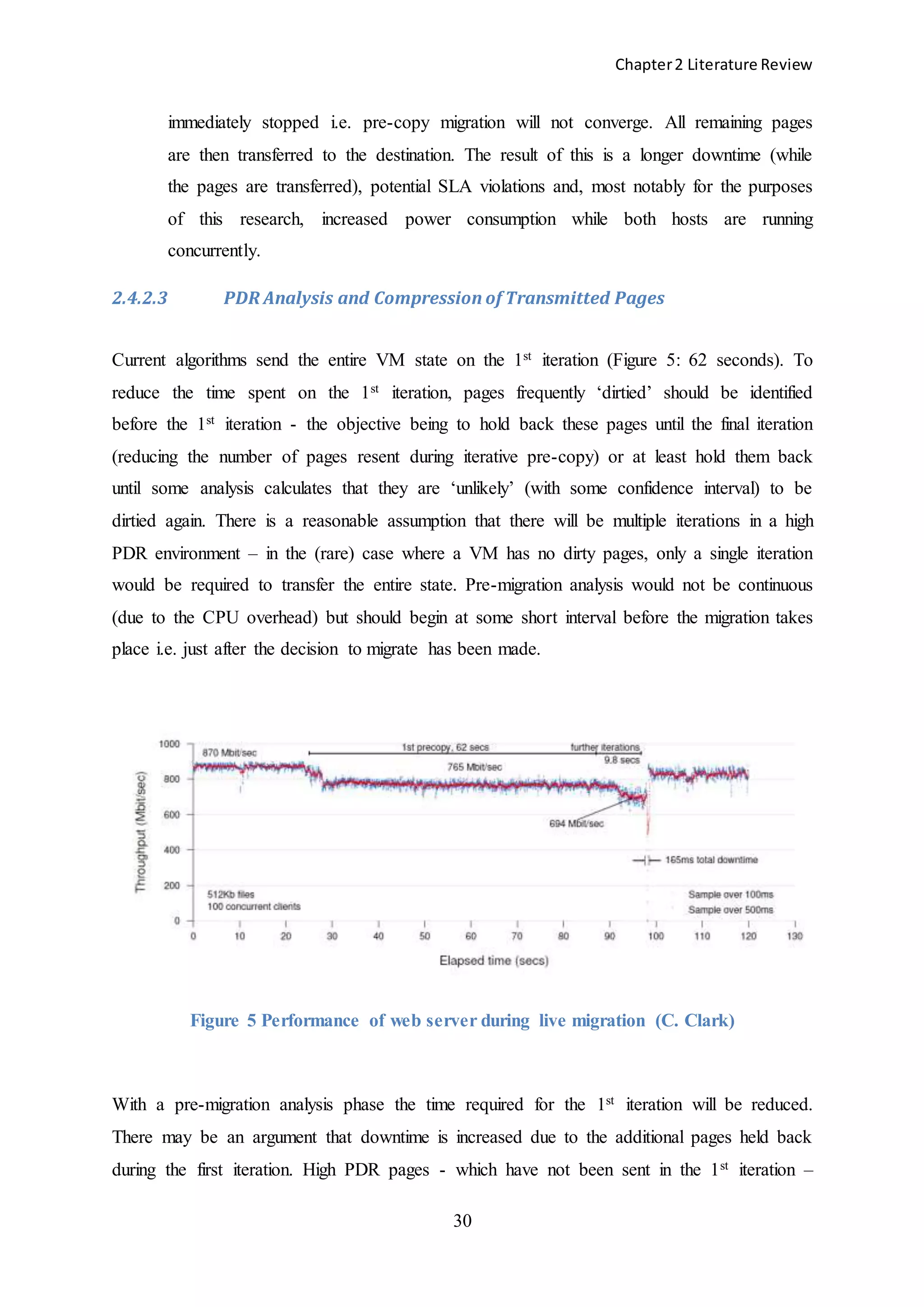
may not converge at all. The PDR floods I/O and the pre-copy migration must be](https://image.slidesharecdn.com/f4c2c6b1-e792-48ec-a4d9-218ade73102c-150302055057-conversion-gate01/75/The-Impact-of-Dynamic-Monitoring-Interval-Adjustment-on-Power-Consumption-in-Virtualized-Data-Centers-37-2048.jpg)
![Chapter2 Literature Review
33
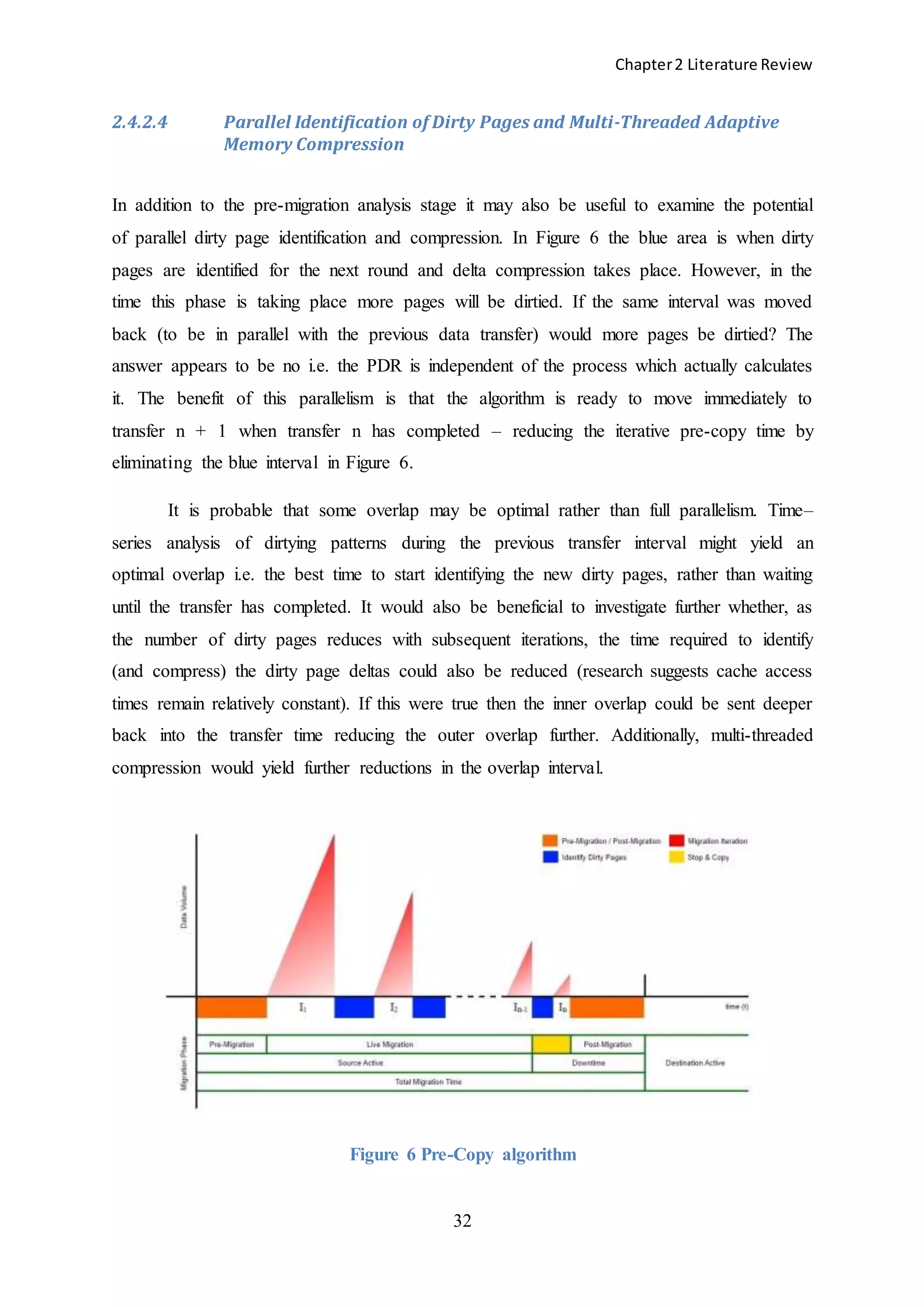
2.4.2.5 Throttling
The critical issue in high PDR environments is that the possibility of convergence is reduced
(if not eliminated altogether). It is similar to a funnel filling up too quickly. If the PDR
continues at a high rate the funnel will eventually overflow resulting in service timeouts i.e.
the application will not respond to subsequent requests or response times will be significantly
decreased. The current solution is to abandon pre-copy migration, stop the VM and transfer
all memory i.e. empty the funnel. Unfortunately, in the time it takes to empty the funnel,
more pages have been dirtied because requests to the application do not stop. This may
actually prohibit the migration altogether because the downtime is such that an unacceptable
level of SLA violations occur.
If, however, the speed at which the application’s response thread can be artificially
slowed down (throttled) intermittently then the funnel is given a better chance to empty its
current contents. This would be analogous to temporarily decreasing the flow from the tap to
reduce the volume in the funnel.
Previous solutions suggested that slowing response time to requests (known as
Dynamic Rate Limiting) would alter the rate at which I/O throughput was performed but
results proved that detrimental VM degradation tended to occur. In addition, other processes
on the same physical machine were negatively affected. Dedicated migration switches were
required to divert the additional load from the core. The focus was on the I/O throughput as
opposed to the incoming workload (PDR).
How the PDR could be intermittently throttled without adverse degradation of either
the VM in question, or other machine processes, is the central question.
Successful PDR throttling, in conjunction with threshold calculations and optimized
parallel adaptive memory compression / dirty page identification, would achieve a lower
PDR. However, the issue of PDR can be essentially circumvented if the number of migrations
taking place in a DC as a whole can be reduced.
In the majority of typical PDR environments Clark et al. [39] have shown that the
initial number of dirty pages i.e. the Writable Working Set (WWS), is a small proportion of
the entire page set (perhaps 10% or less) which needs to be transferred, typically resulting in
minimal iterations being required before a stop condition is reached i.e. subsequent iterations](https://image.slidesharecdn.com/f4c2c6b1-e792-48ec-a4d9-218ade73102c-150302055057-conversion-gate01/75/The-Impact-of-Dynamic-Monitoring-Interval-Adjustment-on-Power-Consumption-in-Virtualized-Data-Centers-41-2048.jpg)
![Chapter2 Literature Review
34
would yield diminishing returns. This is not the case where an application may be particularly
memory-intensive i.e. the PDR is diabolical.
Degradation of application performance during live migration (due to DPDRs or for
other reasons) results in increased response times, threatening violation of SLAs and
increasing power consumption. For optimization of migration algorithms with DPDRs there
are 2 possible approaches for solving the DPDR problem:
1. Increase bandwidth
2. Decrease PDR
Typical applications only exhibit this DPDR-like behaviour as spikes or outliers in normal
write activity. Live migration was previously abandoned by commercial algorithms when
DPDRs were encountered. However, in its most recent version of vSphere (5.0), VMWare
has included an enhancement called ‘Stun During Page Send’ (SDPS) [40] which guarantees
that the migration will continue despite experiencing a DPDR (VMWare refers to DPDRs as
‘pathological’ loads). Tracking both the transmission rate and the PDR, a diabolical PDR can
be identified. When a DPDR is identified by VMWare, the response time of the virtual
machine is slowed down (‘stunned’) by introducing microsecond delays (sleep processes) to
the vCPU. This lowers the response time to application requests and thus slows the rate of
PDR to less than the migration bandwidth (in order to ensure convergence (PDR <
bandwidth).
Xen implements a simple equivalent – limiting ‘rogue’ processes (other applications
or services running parallel to the migration) to 40 write faults before putting them on a wait
queue.
2.5 Monitoring Interval
Much effort has been applied to optimizing the live migration process in recent years. During
migration, the primary factors impacting on a VM’s response SLA are the migration time
and, perhaps more importantly, the downtime. These are the metrics which define the
efficiency of a migration. If a DC operator intends to migrate the VM(s) hosting a client
application it must factor these constraints into its SLA guarantee. It is clear that every
possible effort should be made to minimize the migration time (and downtime) - so that the](https://image.slidesharecdn.com/f4c2c6b1-e792-48ec-a4d9-218ade73102c-150302055057-conversion-gate01/75/The-Impact-of-Dynamic-Monitoring-Interval-Adjustment-on-Power-Consumption-in-Virtualized-Data-Centers-42-2048.jpg)
![Chapter2 Literature Review
35
best possible SLAs may be offered to clients. This can only be achieved by choosing the VM
with the lowest potential PDR for each migration.
However, response and uptime SLAs become increasingly difficult to maintain if
reduction (or at least minimization) of power consumption is a primary objective because
each migration taking place consumes additional energy (while both servers are running and
processing cycles, RAM, bandwidth are being consumed). Based on this premise, Voorsluys
et al. [41] evaluate the cost of live migration, demonstrating that DC power consumption can
be reduced if there is a reduction in migrations. The cost of a migration (as shown) is
dependent on a number of factors, including the amount of RAM being used by the source
VM (which needs to be transferred to the destination) and the bandwidth available for the
migration. The higher the bandwidth the faster data can be transferred. Additionally, power
consumption is increased because 2 VMs (source and destination) are running concurrently
for much of the migration process.
In order to reduce the migration count in a DC each migration should be performed
under the strict condition that the destination host is chosen such that power consumption in
the DC is minimized post-migration. This can only be achieved by examining all possible
destinations before each migration begins - to identify the optimal destination host for each
migrating VM from a power consumption point-of-view. The critical algorithm for resource
(VM) management is the placement algorithm.](https://image.slidesharecdn.com/f4c2c6b1-e792-48ec-a4d9-218ade73102c-150302055057-conversion-gate01/75/The-Impact-of-Dynamic-Monitoring-Interval-Adjustment-on-Power-Consumption-in-Virtualized-Data-Centers-43-2048.jpg)
![Chapter2 Literature Review
36
These 2 conditions i.e.
1. Migrate the VM with the lowest Page Dirty Rate
2. Choose the destination host for minimal power consumption post-migration
form the basis upon which the Local Regression / Minimum Migration Time (LRMMT)
algorithm in CloudSim [42] operates (c.f. Chapter 3).
2.5.1 Static Monitoring Interval
Recent research efforts in energy efficiency perform monitoring of the incoming workload
but almost exclusively focus on techniques for analysis of the data being collected rather than
improving the quality of the data.
In their hotspot identification paper, Xu and Sekiya [43] select a monitoring interval
of 2 minutes. The interval is chosen on the basis of balancing the cost of the additional
processing required against the benefit of performing the migration. The 2 minute interval
remains constant during experimentation.
Using an extended version of the First Fit Decreasing algorithm, Takeda et al. [44]
are motivated by consolidation of servers, to save power. They use a static 60 second
monitoring interval for their work.
Xu and Chen et al. [45] monitor the usage levels of a variety of server resources
(CPU, memory, and bandwidth), polling metrics as often as they become available. Their
results show that monitoring at such a granular level may not only lead to excessive data
processing but the added volume of network monitoring traffic (between multiple hosts and
the monitoring system) may also be disproportionate to the accuracy required.
The processing requirements of DC hosts vary as the workload varies and are not
known until they arrive at the VM, requesting service. While some a priori analysis of the
workload may be performed to predict future demand, as in the work of Gmach et al. [46],
unexpected changes may occur which have not been established by any previously identified
patterns. A more dynamic solution is required which reacts in real-time to the incoming
workload rather than making migration decisions based on a priori analysis.](https://image.slidesharecdn.com/f4c2c6b1-e792-48ec-a4d9-218ade73102c-150302055057-conversion-gate01/75/The-Impact-of-Dynamic-Monitoring-Interval-Adjustment-on-Power-Consumption-in-Virtualized-Data-Centers-44-2048.jpg)
![Chapter2 Literature Review
37
VMware vSphere facilitates a combination of collection intervals and levels [47].
The interval is the time between data collection points and the level determines which metrics
are collected at each interval. Examples of vSphere metrics are as follows:
Collection Interval: 1 day
Collection Frequency: 5 minutes (static)
Level 1 data: 'cpuentitlement', 'totalmhz', 'usage', 'usagemhz'
Level 2 data: 'idle', 'reservedCapacity' + all of Level 1 data (above)
VMware intervals and levels in a DC are adjusted manually by the operator as circumstances
require. Once chosen, they remain constant until the operator re-configures them. Manual
adjustment decisions, which rely heavily on the experience and knowledge of the operator,
may not prove as accurate and consistent over time as an informed, dynamically adjusted
system.
In vSphere, the minimum collection frequency available is 5 minutes. Real-time data
is summarized at each interval and later aggregated for more permanent storage and analysis.
2.5.2 Dynamic Monitoring Interval
Chandra et al. [48] focus on dynamic resource allocation techniques which are sensitive to
fluctuations in data center application workloads. Typically SLA guarantees are managed by
reserving a percentage of available resources (e.g. CPU, network) for each application. The
portion allocated to each application depends on the expected workload and the SLA
requirements of the application. The workload of many applications (e.g. web servers) varies
over time, presenting a significant challenge when attempting to perform a priori estimation
of such workloads. Two issues arise when considering provisioning of resources for web
servers:
1. Over-provisioning based on worst case workload scenarios may result in potential
underutilization of resources e.g. higher CPU priority allocated to application which
seldom requires it
2. Under-provisioning may result in violation of SLAs e.g. not enough CPU priority
given to an application which requires it](https://image.slidesharecdn.com/f4c2c6b1-e792-48ec-a4d9-218ade73102c-150302055057-conversion-gate01/75/The-Impact-of-Dynamic-Monitoring-Interval-Adjustment-on-Power-Consumption-in-Virtualized-Data-Centers-45-2048.jpg)
![Chapter2 Literature Review
38
An alternate approach is to allocate resources to applications dynamically based on
observation of their behaviour in real-time. Any remaining capacity is later allocated to those
applications as and when they are found to require it. Such a system reacts in real-time to
unanticipated workload fluctuations (in either direction), meeting QoS objectives which may
include optimization of power consumption in addition to typical performance SLAs such as
response time.
While Chandra and others [49, 50] have previously used dynamic workload analysis
approaches, their focus was on resource management to optimize SLA guarantees i.e.
performance. No consideration is given in their work to the effect on power consumption
when performance is enhanced. This research differentiates itself in that dynamic analysis of
the workload is performed for the purpose of identifying power consumption opportunities
while also maintaining (or improving) the performance of the DC infrastructure. The search
for improved energy efficiency is driven in this research by DC cost factors which were not as
significant an issue 10-15 years ago as they are now.
2.6 Conclusion
This chapter provided an in-depth analysis of data center energy efficiency state-of-the-art.
Software solutions to energy efficiency issues were presented, demonstrating that many
opportunities still exist for improvement in server room power consumption using a software
approach to monitoring (and control) of the complex systems which comprise a typical DC.
The principle lesson to take from prior (and existing) research in the field is that most of the
DC infrastructure can be monitored using software solutions but that monitoring (and
subsequent processing of the data collected) should not overwhelm the monitoring /
processing system and thus impact negatively on the operation of the DC infrastructure. This
thesis proposes that dynamic adjustment of the monitoring interval with respect to the
incoming workload may represent a superior strategy from an energy efficiency perspective.
Chapter 3 discusses in more detail the capabilities provided by the Java-based CloudSim
framework (used for this research) and the particular code modules relevant to testing the
hypothesis presented herein.](https://image.slidesharecdn.com/f4c2c6b1-e792-48ec-a4d9-218ade73102c-150302055057-conversion-gate01/75/The-Impact-of-Dynamic-Monitoring-Interval-Adjustment-on-Power-Consumption-in-Virtualized-Data-Centers-46-2048.jpg)
![Chapter3 CloudSim
39
Chapter 3 CloudSim
Introduction
Researchers working on data center energy efficiency from a software perspective are
typically hindered by lack of access to real-world infrastructure because it is infeasible to add
additional workload to a data center which already has a significant ‘real-world’ workload to
service on a daily basis. From a commercial perspective, DC operators are understandably
unwilling to permit experimentation on a network which, for the most part, has been fine-
tuned to manage their existing workload. In this chapter, details of the CloudSim framework
are presented with special emphasis on those aspects particularly related to this MSc research
topic.
The CloudSim framework [42] is a Java-based simulator, designed and written by
Anton Beloglazov at the University of Melbourne for his doctoral thesis. It provides a limited
software solution to the above issues and is deployed in this research to simulate a standalone
power-aware data center with LAN-based migration capabilities. The Eclipse IDE is used to
run (and edit) CloudSim.
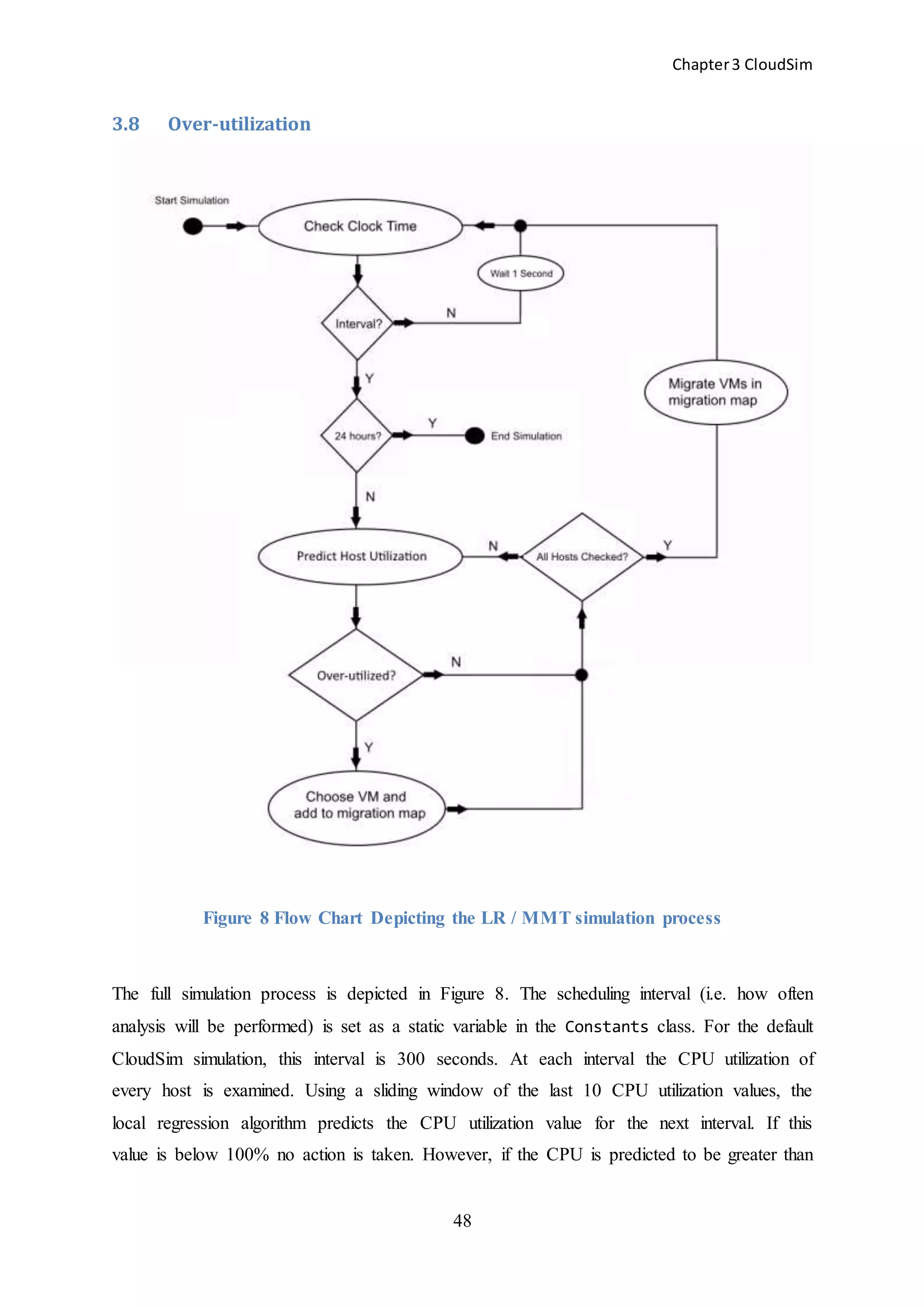
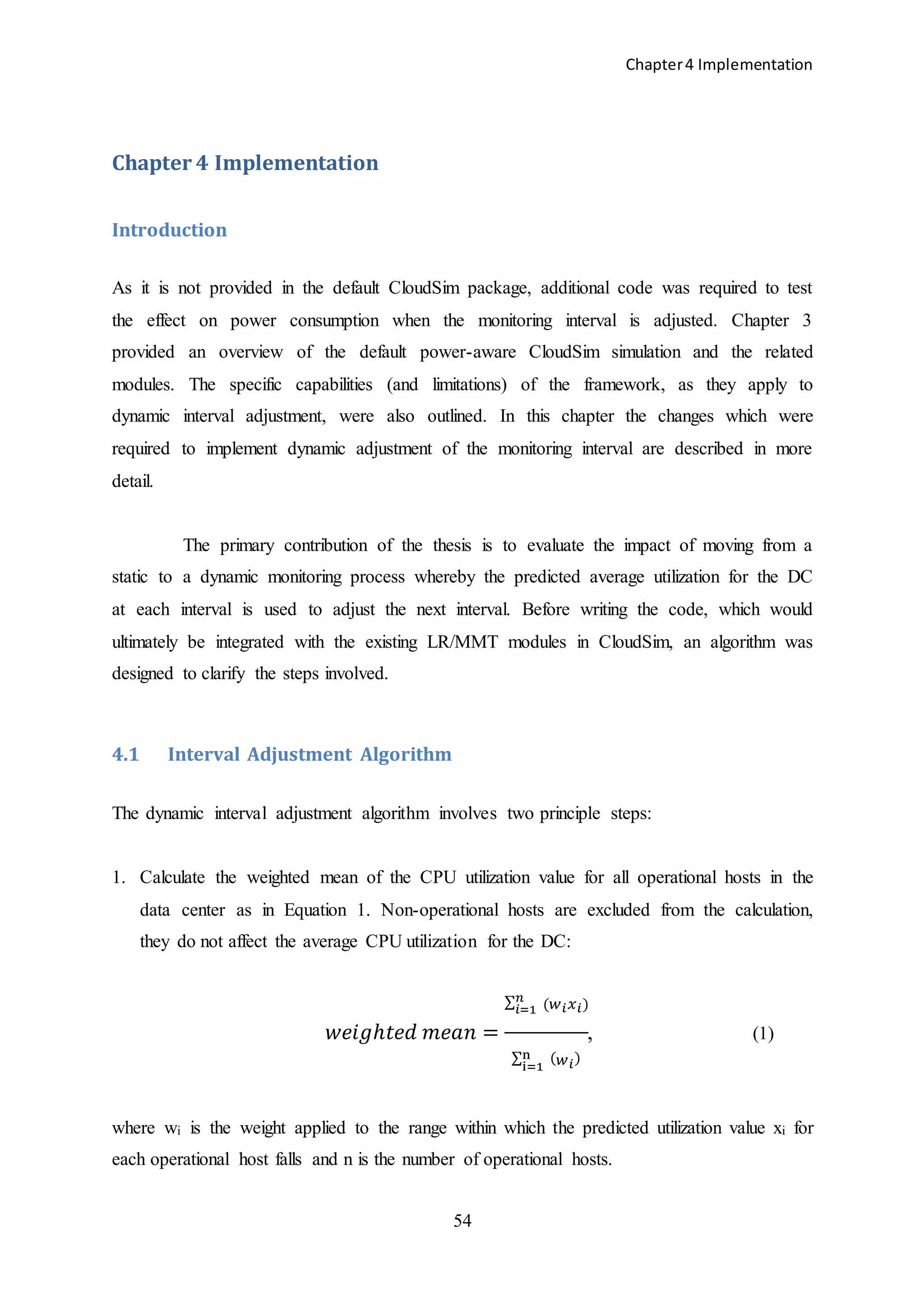
3.1 Overview
Default power-aware algorithms in CloudSim analyse the state of the DC infrastructure at
static 300-second intervals. This reflects current industry practice where an average CPU
utilization value for each host is polled every 5 minutes (i.e. 300 seconds) by virtualization
monitoring systems (e.g. VMware). At each interval the CPU utilization of all hosts in the
simulation is examined to establish whether or not they are adequately servicing the workload
which has been applied to the VMs placed on them.
If a host is found to be over-utilized (i.e. the CPU does not have the capacity to
service the complete workload of all the VMs placed on it) a decision is made to migrate one
or more of the VMs to another host where the required capacity to service the workload is
available.](https://image.slidesharecdn.com/f4c2c6b1-e792-48ec-a4d9-218ade73102c-150302055057-conversion-gate01/75/The-Impact-of-Dynamic-Monitoring-Interval-Adjustment-on-Power-Consumption-in-Virtualized-Data-Centers-47-2048.jpg)
![Chapter3 CloudSim
42
At the beginning of each simulation, the entire cloudlet is loaded into an array
(UtilizationModelPlanetLabInMemory.data[]) from which the values are read at each
interval throughout the simulation. Each cloudlet is assigned to a corresponding VM on a 1-
2-1 basis at the beginning of the simulation.
The values being read from the cloudlets are percentages which simulate ‘real-
world’ CPU utilization values. These need to be converted to a variable in CloudSim which is
related to actual work performed. CloudSim work performance is defined in MIs (Million
Instructions). The workload of the cloudlet (termed length) is a constant i.e. 2500 *
SIMULATION_LENGTH (2500 * 86400 = 216,000,000 MIs). CloudSim keeps track of the
VM workload already performed by subtracting the MIs completed during each interval from
the total cloudlet MI length. As such each cloudlet starts at t = 0 seconds with a workload of
216,000,000 MI and this load is reduced according to the work completed at each interval.
To check whether a cloudlet has been fully executed the IsFinished() method is
called at each interval.
// checks whether this Cloudlet has finished or not
if (cl.IsFinished)
{
…
}
final long finish = resList.get(index).finishedSoFar;
final long result = cloudletLength - finish;
if (result <= 0.0)
{
completed = true;
}
From the code tract above it can be seen that when (or if) the VM’s workload (represented by
the cloudletLength variable) is completed during the simulation the VM will be ‘de-
commissioned’.
3.3 Capacity
Each of the 4 VM types used in the CloudSim framework represents a ‘real-world’ virtual
machine. They are assigned a MIPS value (i.e. 500, 1000, 2000, 2500) before the simulation
begins. This value reflects the maximum amount of processing capacity on the host to which](https://image.slidesharecdn.com/f4c2c6b1-e792-48ec-a4d9-218ade73102c-150302055057-conversion-gate01/75/The-Impact-of-Dynamic-Monitoring-Interval-Adjustment-on-Power-Consumption-in-Virtualized-Data-Centers-50-2048.jpg)
![Chapter3 CloudSim
44
basis at the start of the simulation i.e. in a default simulation with 1052 VMs being placed on
800 hosts, the first 800 VMs are applied to the first 800 hosts and the remaining 352 VMs are
allocated to hosts 1 -> 352. Therefore, when the simulation starts, 352 hosts have 2 VMs and
the remainder host a single VM.
As processing continues the VM placement algorithm attempts to allocate as many
VMs to each host as capacity will allow. The remaining (empty) hosts are then powered off -
simulating the server consolidation effort typical of most modern DCs. It is clear that there is
a conflict of interests taking place. On the one hand there is an attempt to maximize
performance by migrating VMs to hosts with excess capacity but, on the other hand,
competition for CPU cycles is being created by co-locating VMs on the same host,
potentially creating an over-utilization scenario.
3.4 Local Regression / Minimum Migration Time (LR / MMT)
Beloglazov concludes from his CloudSim experiments that the algorithm which combines
Local Regression and Minimum Migration Time (LR / MMT) is most efficient for
maintaining optimal performance and maximizing energy efficiency. Accordingly this
research uses the LR / MMT algorithmic combination as the basis for test and evaluation.
3.5 Selection Policy – Local Regression (LR)
Having passed the most recent CPU utilization values through the Local Regression (LR)
algorithm, hosts are considered over-utilized if the next predicted utilization value exceeds
the threshold of 100% [Appendix A]. LR predicts this value using a sliding window, each
new value being added at each subsequent interval throughout the simulation. The size of the
sliding window is 10. Until initial filling of the window has taken place (i.e. 10 intervals have
elapsed since the simulation began), CloudSim relies on a 'fallback' algorithm [Appendix A]
which considers a host to be over-utilized if its CPU utilization exceeds 70%.
VMs are chosen for migration according to MMT i.e. the VM with the lowest
predicted migration time will be selected for migration to another host. Migration time is
based on the amount of RAM being used by the VM. The VM using the least RAM will be](https://image.slidesharecdn.com/f4c2c6b1-e792-48ec-a4d9-218ade73102c-150302055057-conversion-gate01/75/The-Impact-of-Dynamic-Monitoring-Interval-Adjustment-on-Power-Consumption-in-Virtualized-Data-Centers-52-2048.jpg)
![Chapter3 CloudSim
45
chosen as the primary candidate for migration, simulating minimization of the Dirty Page
Rate (DPR) during VM transfer [39] as previously discussed in Section 2.4.2.2.
3.6 Allocation Policy – Minimum Migration Time (MMT)
The destination host for the migration is chosen on the basis of power consumption following
migration i.e. the host with the lowest power consumption (post migration) is chosen as the
primary destination candidate. In some cases, more than one VM may require migration to
reduce the host's utilization below the threshold. Dynamic RAM adjustment is not facilitated
in CloudSim as the simulation proceeds. Rather, RAM values are read (during execution of
the MMT algorithm) on the basis of the initial allocation to each VM at the start of the
simulation.
3.7 Default LRMMT
The LRMMT algorithm begins in the main() method of the LrMmt.java class [Appendix B].
A PlanetLabRunner() object is instantiated. The PlanetLabRunner() class inherits from
the RunnerAbstract() class and sets up the various parameters required to run the LRMMT
simulation. The parameters are passed to the initLogOutput() method in the default
constructor of the super class (RunnerAbstract) which creates the folders required for
saving the results of the simulation. Two methods are subsequently called:
3.7.1 init()
Defined in the sub-class (PlanetLabRunner), this method takes the location of the PlanetLab
workload (string inputFolder) as a parameter and initiates the simulation. A new
DatacenterBroker() object is instantiated. Among other responsibilities, the broker will
create the VMs for the simulation, bind the cloudlets to those VMs and assign the VMs to the
data center hosts. The broker’s ‘id’ is now passed to the createCloudletListPlanetLab()
method which prepares the cloudlet files in the input folder for storage in a data[288] array.
It is from this array that each cloudlet value will be read so that an equivalent MI workload
value can be calculated for each VM. Having created the cloudletList, the number of
cloudlets (files) in the PlanetLab folder is now known and a list of VMs can be created with
each cloudlet being assigned to an individual VM i.e. there is a 1-2-1 relationship between a
cloudlet and a VM at the start of the simulation. The last call of the init() method creates a](https://image.slidesharecdn.com/f4c2c6b1-e792-48ec-a4d9-218ade73102c-150302055057-conversion-gate01/75/The-Impact-of-Dynamic-Monitoring-Interval-Adjustment-on-Power-Consumption-in-Virtualized-Data-Centers-53-2048.jpg)
![Chapter3 CloudSim
50
3.9 Migration
One or more VMs need to be migrated from the host in order to bring the CPU utilization
back below the threshold. The VM(s) to be migrated are chosen on the basis of the amount of
RAM they are using. Thus, the VM with the least RAM will be the primary candidate for
migration. The VM types used by CloudSim are listed below. It can be seen that (for the most
part †) different RAM values are configured for each VM at the start of the simulation.
CloudSim does not include dynamic RAM adjustment so the static values applied initially
remain the same for the duration. Cloud providers such as Amazon use the term ‘instance’ to
denote a spinning VM. The CloudSim VM types provided simulate some of the VM
instances available to customers in Amazon EC2.
1. High-CPU Medium Instance: 2.5 EC2 Compute Units, 0.85 GB
2. Extra Large Instance: 2 EC2 Compute Units, 3.75 GB †
3. Small Instance: 1 EC2 Compute Unit, 1.7 GB
4. Micro Instance: 0.5 EC2 Compute Unit, 0.633 GB
public final static int VM_TYPES = 4;
public final static int[] VM_RAM = { 870, 1740, 1740†, 613 };
All types are deployed when the VMs are being created at the beginning of the simulation.
Assuming all 4 are on a single host when the host is found to be over-utilized, the order in
which the VMs will be chosen for migration is:
1. 613 [index 3]
2. 870 [index 0]
3. 1740 [index 1]
4. 1740 [index 2] † (note: the VM_RAM value in the default CloudSim code is 1740.
This does not reflect the ‘real-world’ server [Extra Large Instance] being simulated,
which has a RAM value of 3.75 GB)
If there is more than one VM with RAM of 613 on the host they will be queued for migration
before the first ‘870’ enters the queue. The chosen VM is then added to a migration map
which holds a key-value pair of the:](https://image.slidesharecdn.com/f4c2c6b1-e792-48ec-a4d9-218ade73102c-150302055057-conversion-gate01/75/The-Impact-of-Dynamic-Monitoring-Interval-Adjustment-on-Power-Consumption-in-Virtualized-Data-Centers-58-2048.jpg)

![Chapter4 Implementation
56
However, if the minimum interval of 30 seconds was applied for the full 24 hour simulation,
2880 values would be required (i.e. (60 x 60 x 24) / 30) in each PlanetLab cloudlet file to
ensure a value could be read at each interval. The 288 values in the 1052 default files
provided by CloudSim were thus concatenated (using a C# program written specifically for
this purpose) to ensure sufficient values were available, resulting in a total of 105 complete
files with 2880 values each.
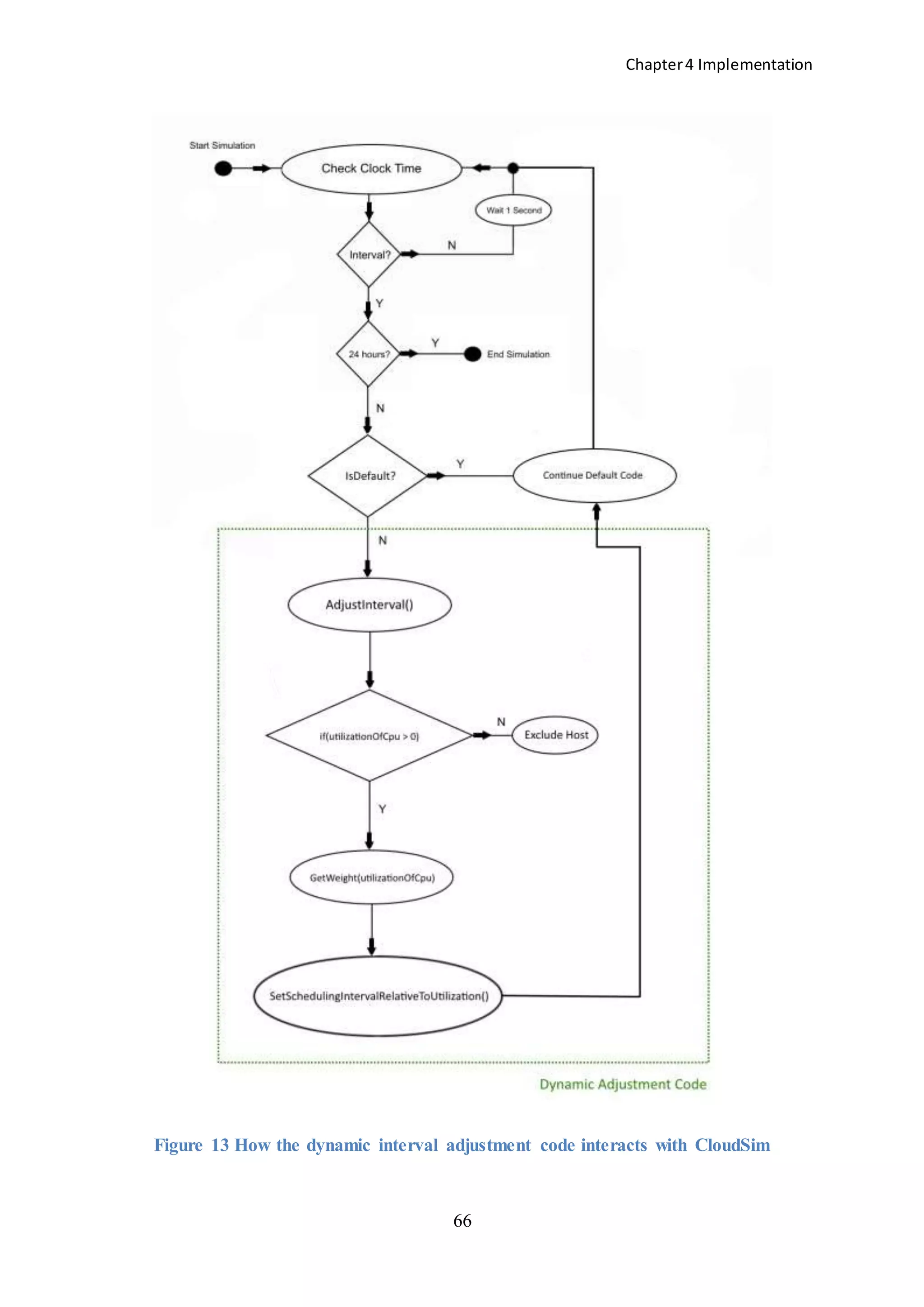
if(Constants.IsDefault)
{
data = new double[288]; // PlanetLab workload
}
else
{
data = new double[2880];
}
The code tract above demonstrates the difference between the two data[] arrays which hold
the PlanetLab cloudlet values read at each interval during the simulation. The default array
is 288 in length while the dynamic is 2880 – providing sufficient indices in the array to store
the required number of cloudlet values throughout the simulation.](https://image.slidesharecdn.com/f4c2c6b1-e792-48ec-a4d9-218ade73102c-150302055057-conversion-gate01/75/The-Impact-of-Dynamic-Monitoring-Interval-Adjustment-on-Power-Consumption-in-Virtualized-Data-Centers-64-2048.jpg)
![Chapter4 Implementation
61
accumulated = (int) Constants.accumulatedIntervals -
_(int) dInterval;
}
Constants.offsetBelow = 300 - accumulated;
Constants.offsetAbove = Constants.accumulatedIntervals - 300;
}
}
4.3 C# Calculator
Calculation of the new per-interval workloads was achieved using a separate ‘calculator’
program written in C#. The calculator implements the process depicted in Figure 12. The
principle C# method used to calculate the new averages for the default files in the calculator
program is CreateDefaultFiles(). The comments in the code explain each step of the
process:
private void CreateDefaultFiles()
{
//read in first 727 from each file - used in dynamic simulation
FileInfo[] Files = dinfo.GetFiles();
string currentNumber = string.Empty;
int iOffsetAboveFromPrevious = 0;
//initialize at max to ensure not used on first iteration
int iIndexForOffsetAbove = 727;
foreach (FileInfo filex in Files)
{
using (var reader = new StreamReader(filex.FullName))
{
//fill dynamicIn
for (int i = 0; i < 727; i++)
{
dynamicIn[i] = Convert.ToInt32(reader.ReadLine());
}
int iCurrentOutputIndex = 0;
//Calculate
for (int k = 0; k < 727; k++)
{
//add each average used here - including any offset
float iAccumulatedTotal = 0;
//reached > 300 accumulated intervals
int iReadCount =
_Convert.ToInt32(ds.Tables[0].Rows[k]["ReadCount"]);](https://image.slidesharecdn.com/f4c2c6b1-e792-48ec-a4d9-218ade73102c-150302055057-conversion-gate01/75/The-Impact-of-Dynamic-Monitoring-Interval-Adjustment-on-Power-Consumption-in-Virtualized-Data-Centers-69-2048.jpg)
![Chapter4 Implementation
62
if (iReadCount > 0)
{
//first interval
if (k == 0)
{
int iValue = dynamicIn[k];
iAccumulatedTotal += iValue;
}
else
{
//readCount == 1: just check for offsets
if (iReadCount > 1)
{
for (int m = 1; m < iReadCount; m++)
{
int iValue = dynamicIn[k - m];
int iInterval =
_Convert.ToInt32(ds.Tables[0].Rows[k - _m]["Interval"]);
iAccumulatedTotal += iValue * iInterval;
}
}
}
//offset - read this interval
int iOffsetBelow =
_Convert.ToInt32(ds.Tables[0].Rows[k]["OffsetBelow300"]);
if (iOffsetBelow > 0)
{
iAccumulatedTotal += iOffsetBelow * dynamicIn[k];
}
//use previous offset above in this calculation
if (k >= iIndexForOffsetAbove)
{
iAccumulatedTotal += iOffsetAboveFromPrevious;
//reset
iOffsetAboveFromPrevious = 0;
iIndexForOffsetAbove = 727;
}
//use this offset above in next calculation
int iOffsetAbove =
_Convert.ToInt32(ds.Tables[0].Rows[k]["OffsetAbove300"]);
if (iOffsetAbove > 0)
{
//value for offset above to add to next
_accumulator
iOffsetAboveFromPrevious = iOffsetAbove *
_dynamicIn[k];
//use in next calculation - at a minimum
iIndexForOffsetAbove = k;
}](https://image.slidesharecdn.com/f4c2c6b1-e792-48ec-a4d9-218ade73102c-150302055057-conversion-gate01/75/The-Impact-of-Dynamic-Monitoring-Interval-Adjustment-on-Power-Consumption-in-Virtualized-Data-Centers-70-2048.jpg)
![Chapter4 Implementation
63
float fAverage = iAccumulatedTotal / 300;
int iAverage = Convert.ToInt32( iAccumulatedTotal /
_300);
//first interval
if (k == 0)
{
iAverage = dynamicIn[k];
}
//save averaged value to array for writing
defaultOutput[iCurrentOutputIndex] =
_iAverage.ToString();
iCurrentOutputIndex++;
}
}
}
//Print to text file for default cloudlet
System.IO.File.WriteAllLines("C:UsersscoobyDesktopDefaultNewFiles
" + _filex.Name, defaultOutput);
}
}
The code above depicts the process by which the values required to calculate the default file
averages was achieved. Having run the dynamic simulationThe results of the calculator
program were written back out to flat text files i.e. the same format as the original CloudSim
cloudlet files. To compare the difference between the default and dynamic workloads, both
default and dynamic simulations were run using the new cloudlet files with a few lines of
additional code to monitor the workload during each simulation added to the default
constructor of the UtilizationModelPlanetlabInMemory() class in CloudSim. This
additional code ensured that the workload would be observed (and accumulated) as each
cloudlet was processed.
As the data is being read into the data[] array from the PlanetLab cloudlet files
each value is added to a new accumulator variable i.e. Constants.totalWorkload:
int n = data.length;
for (int i = 0; i < n - 1; i++)
{
data[i] = Integer.valueOf(input.readLine());
Constants.totalWorkload += data[i];
}](https://image.slidesharecdn.com/f4c2c6b1-e792-48ec-a4d9-218ade73102c-150302055057-conversion-gate01/75/The-Impact-of-Dynamic-Monitoring-Interval-Adjustment-on-Power-Consumption-in-Virtualized-Data-Centers-71-2048.jpg)
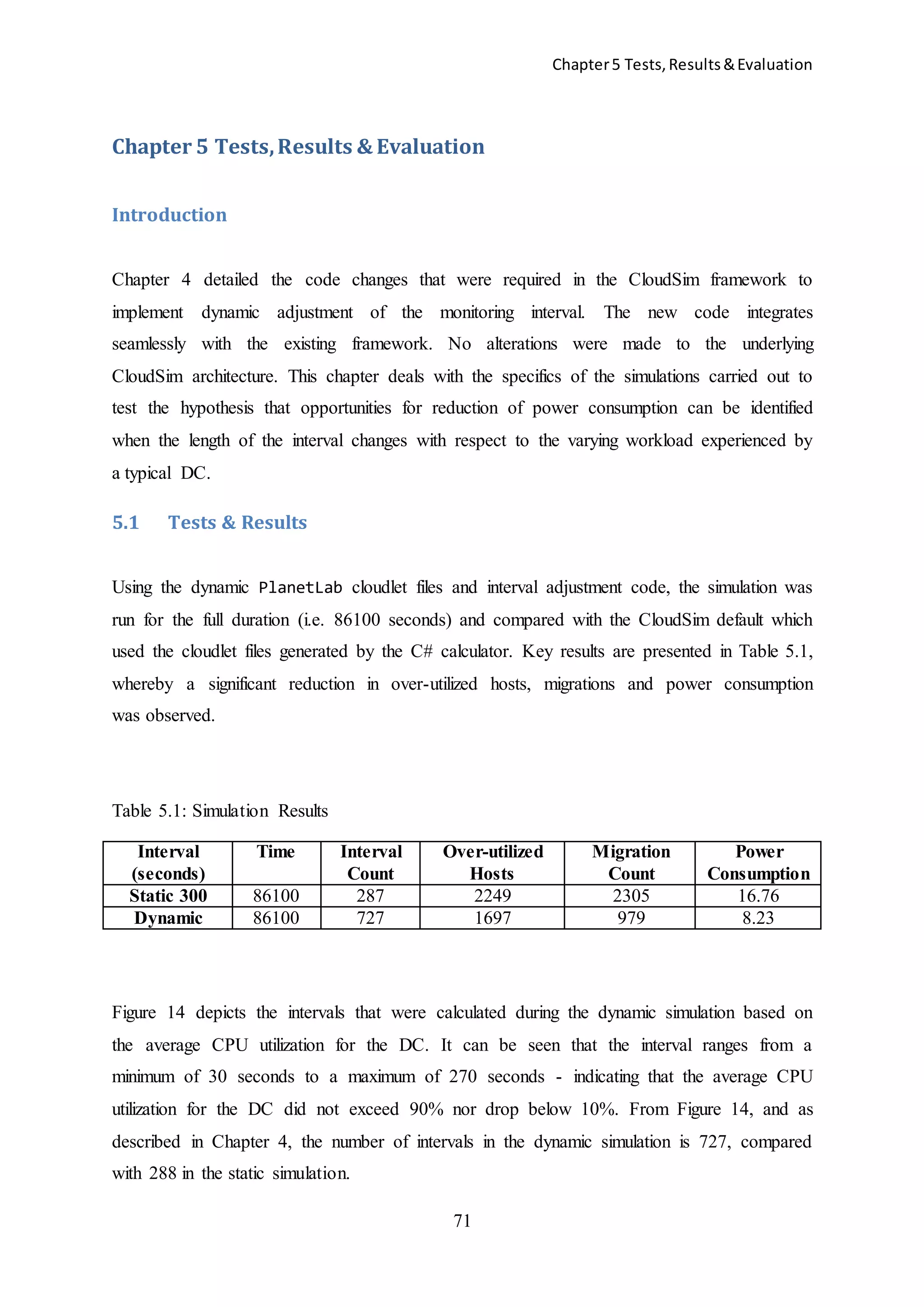

![Chapter5 Tests,Results&Evaluation
77
5.2.2 Result of Reduced Migration Count
Beloglazov et al. [51] show that decreased power consumption can be achieved in a DC if the
VM migration count can be reduced. Their work is based on the premise that additional
resources are consumed during a migration due to the extra processing required to move the
memory of the VM from its current host to another. Those processes may include:
Identification of a suitable destination server i.e. VM placement algorithm
Network traffic
CPU processing on both source and destination servers whilst concurrently running
two VMs
In the case of live migration, transfer of the VM’s memory image is performed by the Virtual
Machine Manager (VMM) which copies the RAM, associated with the VM service, across to
the destination while the service on the VM is still running. RAM which is re-written on the
source must be transferred again. This process continues iteratively until the remaining
volume of RAM needing to be transferred is such that the service can be switched off with
minimal interruption. This period of time, while the service is unavailable, is known as
downtime. Any attempt to improve migration algorithms must take live-copy downtime into
consideration to prevent (or minimize) response SLAs. CloudSim achieves this (to some
extent) by choosing, for migration, the VM with the lowest RAM. However, the CloudSim
SLA metric in the modules used for this research does not take this downtime into
consideration.
Dynamic adjustment of the monitoring interval, however, minimizes this issue of
RAM transfer by reducing the need for the migration in the first place. The power consumed
as a result of the migrations is saved when additional migrations are not required.
5.2.3 Scalability
As outlined in Section 2.1 there is a trade-off between DC monitoring overhead costs and net
DC benefits. The issue here is that the additional volume of processing which takes place
when shorter monitoring intervals are applied may become such that it would not be
beneficial to apply dynamic interval adjustment at all.](https://image.slidesharecdn.com/f4c2c6b1-e792-48ec-a4d9-218ade73102c-150302055057-conversion-gate01/75/The-Impact-of-Dynamic-Monitoring-Interval-Adjustment-on-Power-Consumption-in-Virtualized-Data-Centers-85-2048.jpg)
![Chapter5 Tests,Results&Evaluation
78
Take for example, Amazon’s EC2 EU West DC (located in Dublin, Ireland) which is
estimated to contain over 52,000 operational servers [52]. Processing of the data (CPU
utilization values) required to perform the interval adjustment is not an insignificant
additional workload. The algorithm will calculate the average CPU utilization of some 52,000
servers and apply the new interval. As such, if this calculation were to take place every 30
seconds (in a DC with an average CPU utilization above 90%), rather than every 300
seconds, there is a ten-fold increase in the total processing volume which includes both
collection and analysis of the data points. While it is unlikely that even the average CPU
utilization of the most efficient DC would exceed 90% for any extended period of time, it is
clear that the size of the DC (i.e. number of operational servers) does play a role in
establishing whether or not the interval adjustment algorithm described in this research
should be applied. Microsoft’s Chicago DC has approximately 140,000 servers installed.
With increasingly larger DCs being built to meet growing consumer demand, it is reasonable
to expect that DC server counts will reach 500,000 in the foreseeable future. Rather than
viewing the entire DC as a single entity from a monitoring perspective, perhaps the most
viable application of dynamic monitoring interval adjustment would be to sub-divide these
larger DCs into more manageable sections, calculating the monitoring interval for each
section separately.
5.3 Evaluation of CloudSim
5.3.1 Local Regression Sliding Window
The adjusted interval in this research (discussed in Chapter 3 Section 5) results in the 'first
fill' of the window occurring sooner than the CloudSim default i.e. the longest interval (5
minutes) in the dynamic version is the minimum (static) interval in the CloudSim default.
The first 10 values in the sliding window take 3000 seconds (i.e. 300 x 10) in the default
CloudSim simulation whereas, in the dynamic version, the window is filled after 1480
seconds. The result is a small increase in the accuracy of the utilization prediction at the
beginning of the simulation because the less accurate ‘fallback’ algorithm is ‘discarded’
sooner.
The size of the sliding window in the default CloudSim framework is 10 i.e. the 10 most
recent CPU utilization values from the host are used each time the local regression algorithm](https://image.slidesharecdn.com/f4c2c6b1-e792-48ec-a4d9-218ade73102c-150302055057-conversion-gate01/75/The-Impact-of-Dynamic-Monitoring-Interval-Adjustment-on-Power-Consumption-in-Virtualized-Data-Centers-86-2048.jpg)
![Chapter6 Conclusions
82
prove both informative and useful for researchers undertaking CloudSim-based simulations in
the future.
Recent reports suggest that Microsoft’s Chicago DC has approximately 140,000
servers installed [53]. With increasingly larger DCs being built to meet growing consumer
demand, it is reasonable to expect that individual DC server counts will reach 250,000 -
500,000 in the foreseeable future. Rather than viewing the entire DC as a single entity from a
monitoring perspective, perhaps the most viable application of dynamic monitoring interval
adjustment would be to sub-divide these larger DCs into more manageable sections,
calculating (and adjusting) the monitoring interval for each section separately – ensuring that
the granularity of analysis most appropriately caters for all possible data center sizes and
configurations. This analysis would also make a valuable contribution to the state-of-the-art.](https://image.slidesharecdn.com/f4c2c6b1-e792-48ec-a4d9-218ade73102c-150302055057-conversion-gate01/75/The-Impact-of-Dynamic-Monitoring-Interval-Adjustment-on-Power-Consumption-in-Virtualized-Data-Centers-90-2048.jpg)
![References
83
REFERENCES
[1] http://www.gartner.com/newsroom/id/499090 - last accessed on 19/09/2014
[2] http://www.idc.com - last accessed on 19/09/2014
[3] Koomey J.G., “Estimating Total Power Consumption by Servers in the U.S. and the
World”, 2007
[4] Energy Star Program - U.S. Environmental Protection Agency, “EPA Report to Congress
on Server and Data Center Energy Efficiency”, EPA, Aug 2007.
[5] N. Rasmussen, “Calculating Total Cooling Requirements for Data Centers,” American
Power Conversion, White Paper #25, 2007.
[6] Sharma, R.K.; Bash, C.E.; Patel, C.D.; Friedrich, R.J.; Chase, J.S., "Balance of Power:
Dynamic Thermal Management for Internet Data Centers," Internet Computing, IEEE, vol.9,
no.1, pp. 42-49, January 2005
[7] Moore, J.; Sharma, R.; Shih, R.; Chase, J.; Patel, C.; Ranganathan, P., “Going Beyond
CPUs: The Potential of Temperature-Aware Solutions for the Data Center”, Hewlett Packard
Labs, 2002
[8] Data Center Efficiency Task Force, “Recommendations for Measuring and Reporting
Version 2 – Measuring PUE for Data Centers”, 17th May 2011
[9] C. Belady, A., Rawson, J. Pfleuger, and T., Cader, "Green Grid Data Center Power
Efficiency Metrics: PUE and DCIE," The Green Grid, 2008
[10] Koomey J.G., “Growth in Data Center Electricity Use 2005 to 2010”, report by
Analytics Press, completed at the request of The New York Times, August 2011
[11] The Uptime Institute, “Inaugural Annual Uptime Institute Data Center Industry Survey”,
Uptime Institute, May 2011
[12] ASHRAE, “Datacom Equipment Power Trends and Cooling Applications”, ASHRAE
INC, 2005](https://image.slidesharecdn.com/f4c2c6b1-e792-48ec-a4d9-218ade73102c-150302055057-conversion-gate01/75/The-Impact-of-Dynamic-Monitoring-Interval-Adjustment-on-Power-Consumption-in-Virtualized-Data-Centers-91-2048.jpg)
![References
84
[13] ASHRAE, "Environmental Guidelines for Datacom Equipment - Expanding the
Recommended Environmental Envelope", ASHRAE INC, 2008
[14] ASHRAE, “Thermal Guidelines for Data Processing Environments – Expanded Data
Center Classes and Usage Guidance”, ASHRAE INC, August 2011
[15] Boucher, T.D.; Auslander, D.M.; Bash, C.E.; Federspiel, C.C.; Patel, C.D., "Viability of
Dynamic Cooling Control in a Data Center Environment," Thermal and Thermomechanical
Phenomena in Electronic Systems, 2004. ITHERM '04. The Ninth Intersociety Conference
on, pp. 593- 600 Vol. 1, 1-4 June 2004
[16] Sharma, R.K.; Bash, C.E.; Patel, C.D.; Friedrich, R.J.; Chase, J.S.; , "Balance of Power:
Dynamic Thermal Management for Internet Data Centers," Internet Computing, IEEE , vol.9,
no.1, pp. 42- 49, Jan.-Feb. 2005
[17] Shah, A.; Patel, C.; Bash, C.; Sharma, R.; Shih, R.; , "Impact of Rack-level Compaction
on the Data Center Cooling Ensemble," Thermal and Thermomechanical Phenomena in
Electronic Systems, 2008. ITHERM 2008. 11th Intersociety Conference on, pp.1175-1182,
28-31 May 2008
[18] C. Patel, et al., “Energy Flow in the Information Technology Stack: Coefficient of
Performance of the Ensemble and its Impact on the Total Cost of Ownership,” Technical
Report No. HPL-2006-55, Hewlett Packard Laboratories, March 2006
[19] C. Patel, et al., “Energy Flow in the Information Technology Stack: Introducing the
Coefficient of Performance of the Ensemble,” Proc. ASME IMECE, November 2006
[20] Ahuja, N.; Rego, C.; Ahuja, S.; Warner, M.; Docca, A.; "Data Center Efficiency with
Higher Ambient Temperatures and Optimized Cooling Control," Semiconductor Thermal
Measurement and Management Symposium (SEMI-THERM), 2011 27th Annual IEEE,
pp.105-109, 20-24 March 2011
[21] Berktold, M.; Tian, T., “CPU Monitoring With DTS/PECI”, Intel Corporation,
September 2010
[22] M. Stopar, SLA@SOI XLAB, Efficient Distribution of Virtual Machines, March 24,
2011.](https://image.slidesharecdn.com/f4c2c6b1-e792-48ec-a4d9-218ade73102c-150302055057-conversion-gate01/75/The-Impact-of-Dynamic-Monitoring-Interval-Adjustment-on-Power-Consumption-in-Virtualized-Data-Centers-92-2048.jpg)
![References
85
[23] C. Hyser, B. McKee, R. Gardner, and B. Watson. Autonomic Virtual Machine
Placement in the Data Center. Technical Report HPL-2007-189, HP Laboratories, Feb. 2008.
[24] A. Qureshi, R. Weber, H. Balakrishnan, J. Guttag, and B. Maggs, “Cutting the Electric
Bill for Internet-Scale Systems,” in Proc. ACM Conference on Data Communication
(SIGCOMM’09), New York, NY, USA, 2009, pp. 123–134
[25] Bolin Hu; Zhou Lei; Yu Lei; Dong Xu; Jiandun Li; , "A Time-Series Based Precopy
Approach for Live Migration of Virtual Machines," Parallel and Distributed Systems
(ICPADS), 2011 IEEE 17th International Conference on , vol., no., pp.947-952, 7-9 Dec.
2011
[26] Carroll, R, Balasubramaniam, S, Botvich, D and Donnelly, W, Application of Genetic
Algorithm to Maximise Clean Energy usage for Data Centers, to appear in proceedings of
Bionetics 2010, Boston, December 2010
[27] Akshat Verma, Puneet Ahuja, Anindya Neogi, “pMapper: Power and Migration Cost
Aware Application Placement in Virtualized Systems”, Middleware 2008: 243-264
[28] P. Riteau, C. Morin, T. Priol, “Shrinker: Efficient Wide-Area Live Virtual Machine
Migration using Distributed Content-Based Addressing,”
http://hal.inria.fr/docs/00/45/47/27/PDF/RR-7198.pdf, 2010
[29] F. Travostino, P. Daspit, L. Gommans, C. Jog, C. de Laat, J. Mambretti, I. Monga, B.
van Oudenaarde, S. Raghunath, and P. Wang. Seamless Live Migration of Virtual Machines
over the MAN/WAN. iGrid, 2006
[30] Hai Jin, Li Deng, Song Wu, Xuanhua Shi, and Xiaodong Pan. Live virtual machine
migration with adaptive memory compression. In Cluster, 2009
[31] Jonghyun Lee, MarianneWinslett, Xiaosong Ma, and Shengke Yu. Enhancing Data
Migration Performance via Parallel Data Compression. In Proceedings of the 16th
International Parallel and Distributed Processing Symposium (IPDPS), pages 47–54, April
2002
[32] M. R. Hines and K. Gopalan, “Post-copy based live virtual machine migration using
adaptive pre-paging and dynamic self-ballooning,” in Proceedings of the ACM/Usenix
international conference on Virtual execution environments (VEE’09), 2009, pp. 51–60](https://image.slidesharecdn.com/f4c2c6b1-e792-48ec-a4d9-218ade73102c-150302055057-conversion-gate01/75/The-Impact-of-Dynamic-Monitoring-Interval-Adjustment-on-Power-Consumption-in-Virtualized-Data-Centers-93-2048.jpg)
![References
86
[33] Bose, S.K.; Brock, S.; Skeoch, R.; Rao, S.; , "CloudSpider: Combining Replication with
Scheduling for Optimizing Live Migration of Virtual Machines across Wide Area
Networks," Cluster, Cloud and Grid Computing (CCGrid), 2011 11th IEEE/ACM
International Symposium on , vol., no., pp.13-22, 23-26 May 2011
[34] Cioara, T.; Anghel, I.; Salomie, I.; Copil, G.; Moldovan, D.; Kipp, A.; , "Energy Aware
Dynamic Resource Consolidation Algorithm for Virtualized Service Centers Based on
Reinforcement Learning," Parallel and Distributed Computing (ISPDC), 2011 10th
International Symposium on , vol., no., pp.163-169, 6-8 July 2011
[35] H. Liu, H. Jin, X. Liao, L. Hu, and C. Yu, “Live migration of virtual machine based on
full system trace and replay,” in Proceedings of the 18th International Symposium on High
Performance Distributed Computing (HPDC’09), 2009, pp. 101–110.
[36] http://www.drbd.org - last accessed on 19/09/2014
[37] K. Nagin, D. Hadas, Z. Dubitzky, A. Glikson, I. Loy, B. Rochwerger, and L. Schour,
“Inter-Cloud Mobility of Virtual Machines,” in Proc. of 4th Int’l Conf. on Systems & Storage
(SYSTOR). ACM, 2011, pp. 3:1–3:12.
[38] R. Bradford, E. Kotsovinos, A. Feldmann, and H. Schi•oberg. Live Wide-Area
Migration of Virtual Machines including Local Persistent State. In VEE '07: Proceedings of
the 3rd international conference on Virtual execution environments, pages 169{179, New
York, NY, USA, 2007. ACM.
[39] C. Clark, K. Fraser, A. Hand, J. Hansen, E. Jul, C. Limpach, I. Pratt, A. Warfield. Live
Migration of Virtual Machines. in Proceedings of the Symposium on Networked Systems
Design and Implementation, 2005.
[40] VMware vSphere® vMotion®, Architecture, Performance and Best Practices in
VMware vSphere® 5. Performance Study, Technical White Paper, Oct 2011.
[41] Voorsluys W., Broberg J., Venugopal S., Buyya R.: Cost of Virtual Machine Live
Migration in Clouds: a Performance Evaluation. In: Proceedings of the 1st International
Conference on Cloud Computing. Vol. 2009. Springer (2009)
[42] Buyya, R., Ranjan, R., Calheiros, R. N.: Modeling and Simulation of Scalable Cloud
Computing Environments and the CloudSim Toolkit: Challenges and Opportunities. In: High](https://image.slidesharecdn.com/f4c2c6b1-e792-48ec-a4d9-218ade73102c-150302055057-conversion-gate01/75/The-Impact-of-Dynamic-Monitoring-Interval-Adjustment-on-Power-Consumption-in-Virtualized-Data-Centers-94-2048.jpg)
![References
87
Performance Computing & Simulation, 2009. HPCS'09. International Conference on, pp. 1-
11. IEEE (2009)
[43] Xu, Y., Sekiya, Y.: Scheme of Resource Optimization using VM Migration for
Federated Cloud. In: Proceedings of the Asia-Pacific Advanced Network, vol. 32, pp. 36-44.
(2011)
[44] Takeda, S., and Toshinori T.: A Rank-Based VM Consolidation Method for Power
Saving in Data Centers. IPSJ Online Transactions, vol. 3 pp. 88-96. J-STAGE (2010)
[45] Xu, L., Chen, W., Wang, Z., Yang, S.: Smart-DRS: A Strategy of Dynamic Resource
Scheduling in Cloud Data Center. In: Cluster Computing Workshops (CLUSTER
WORKSHOPS), IEEE International Conference on, pp. 120-127. IEEE (2012)
[46] Gmach, D., Rolia, J., Cherkasova, L., Kemper, A.: Workload Analysis and Demand
Prediction of Enterprise Data Center Applications. In: Workload Characterization, 2007.
IISWC 2007. IEEE 10th International Symposium on, pp. 171-180. IEEE (2007)
[47] VMware, http://pubs.vmware.com/vsphere-4-esx-
vcenter/index.jsp?topic=/com.vmware.vsphere.bsa.doc_40/vc_perfcharts_help/c_perfcharts_c
ollection_intervals.html - last accessed on 19/09/2014
[48] Chandra, A., W. Gong, et al. (2003). Dynamic Resource Allocation for Shared Data
Centers Using Online Measurements. Proceedings of the Eleventh International Workshop on
Quality of Service (IWQoS 2003), Berkeley, Monterey, CA, Springer. pp. 381-400.
[49] M. Aron, P. Druschel, and S. Iyer. A Resource Management Framework for Predictable
Quality of Service in Web Servers, 2001.
[50] J. Carlstrom and R. Rom. Application-Aware Admission Control and Scheduling in Web
Servers. In Proceedings of the IEEE Infocom 2002, June 2002.
[51] Beloglazov, A., and Rajkumar B.: Energy Efficient Resource Management in
Virtualized Cloud Data Centers. Proceedings of the 2010 10th IEEE/ACM International
Conference on Cluster, Cloud and Grid Computing. IEEE Computer Society, 2010.
[52] http://huanliu.wordpress.com/2012/03/13/amazon-data-center-size - last accessed on
19/09/2014](https://image.slidesharecdn.com/f4c2c6b1-e792-48ec-a4d9-218ade73102c-150302055057-conversion-gate01/75/The-Impact-of-Dynamic-Monitoring-Interval-Adjustment-on-Power-Consumption-in-Virtualized-Data-Centers-95-2048.jpg)
![References
88
[53] http://www.datacenterknowledge.com/archives/2009/06/29/microsoft-to-open-two-
massive-data-centers - last accessed on 19/09/2014](https://image.slidesharecdn.com/f4c2c6b1-e792-48ec-a4d9-218ade73102c-150302055057-conversion-gate01/75/The-Impact-of-Dynamic-Monitoring-Interval-Adjustment-on-Power-Consumption-in-Virtualized-Data-Centers-96-2048.jpg)
![Appendices
89
APPENDIX A
The code which checks if a host is over-utilized. The ‘fallback’ algorithm is used until the
sliding window (length = 10) has been filled.
@Override
protected boolean isHostOverUtilized(PowerHost host)
{
PowerHostUtilizationHistory _host = (PowerHostUtilizationHistory)
host;
double[] utilizationHistory = _host.getUtilizationHistory();
int length = 10;
if (utilizationHistory.length < length)
{
return
getFallbackVmAllocationPolicy().isHostOverUtilized(host);
}
double[] utilizationHistoryReversed = new double[length];
for (int i = 0; i < length; i++)
{
utilizationHistoryReversed[i] = utilizationHistory[length - i
- 1];
}
double[] estimates = null;
try
{
estimates = getParameterEstimates(utilizationHistoryReversed);
}
catch (IllegalArgumentException e)
{
return
getFallbackVmAllocationPolicy().isHostOverUtilized(host);
}
double migrationIntervals =
Math.ceil(getMaximumVmMigrationTime(_host) /
Constants.SCHEDULING_INTERVAL);
double predictedUtilization = estimates[0] + estimates[1] * (length
+ migrationIntervals);
predictedUtilization *= getSafetyParameter();
addHistoryEntry(host, predictedUtilization);
if(predictedUtilization >= 1)
{
Constants.OverUtilizedHostsThisInterval++;
}
return predictedUtilization >= 1;
}](https://image.slidesharecdn.com/f4c2c6b1-e792-48ec-a4d9-218ade73102c-150302055057-conversion-gate01/75/The-Impact-of-Dynamic-Monitoring-Interval-Adjustment-on-Power-Consumption-in-Virtualized-Data-Centers-97-2048.jpg)
![Appendices
90
APPENDIX B
The main() method of the LRMMT algorithm.
public static void main(String[] args) throws IOException
{
boolean enableOutput = true;
boolean outputToFile = true;
String inputFolder =
"C:UsersscoobyDesktopEclipseCloudSimexamplesworkloadplanet
lab";
//default workload generated from dynamic averages
String workload = "default";
//dynamic workload
if(!Constants.IsDefault)
{
workload = "dynamic"; // PlanetLab workload
}
if(Constants.IntervalGenerator)
{
Constants.SIMULATION_LIMIT = 86400;
}
String outputFolder =
"C:UsersscoobyDesktopEclipseWorkspaceoutput";
String vmAllocationPolicy = "lr"; // Local Regression (LR) VM
allocation policy
String vmSelectionPolicy = "mmt"; // Minimum Migration Time (MMT) VM
selection policy
String parameter = "1.2"; // the safety parameter of the LR policy
new PlanetLabRunner(enableOutput, outputToFile, inputFolder,
outputFolder, workload, vmAllocationPolicy, _vmSelectionPolicy,
parameter);
}](https://image.slidesharecdn.com/f4c2c6b1-e792-48ec-a4d9-218ade73102c-150302055057-conversion-gate01/75/The-Impact-of-Dynamic-Monitoring-Interval-Adjustment-on-Power-Consumption-in-Virtualized-Data-Centers-98-2048.jpg)

This thesis explores the impact of dynamically adjusting monitoring intervals on power consumption in virtualized data centers, proposing that reduced power usage can be achieved by analyzing performance metrics at appropriate granularity based on CPU utilization. It discusses various aspects of data centers, including energy efficiency, migration, and the CloudSim framework as a simulation tool for power-aware systems. The research aims to highlight the potential operational savings and efficiencies gained from optimizing monitoring strategies in increasingly energy-conscious environments.