This paper aims to analyze potential differences in the temporal patterns of misinformation diffusion compared to factual information diffusion on Twitter. Specifically, it looks at the speed of distribution and whether a lack of evenness in distribution is correlated with misinformation, building on previous research. The researchers found no strong evidence that speed of distribution is directly correlated with validity, but temporal patterns could potentially be used along with other methods to more quickly identify misinformation given the harm it can cause. Understanding how information spreads on social networks is important as both useful and harmful information can diffuse rapidly.

1. Temporal Patterns of Misinformation Diffusion in Online
Social Networks
Analyzing Velocity of Misinformation
Salim Chaouqi
University of Florida
salimc@ufl.edu
Harry Gogonis
University of Florida
hgogonis@gmail.com
Dylan Richardson
University of Florida
dylanrichardson47@gmail.com
ABSTRACT
In this paper, we explored potential temporal differences
between the diffusion of misinformation and information in
Twitter. Additionally, we expanded on Kumar et al.’s re-
search on the correlation between disinformation and lack
of evenness of distribution of that disinformation by testing
their findings on misinformation of a more general level.
We found that there is no strong evidence of direct corre-
lation between speed of distribution of information and its
validity, although there were certain limitations that we ex-
perienced which caused a lack of comprehensive coverage in
terms of the magnitude and diversity of data explored. Ad-
ditionally, the unevenness of distribution of information is
not a property of misinformation to any significant extent,
unlike disinformation. While the property of velocity of in-
formation is not a standalone indicator of the credibility, it
could possibly be utilized in conjunction with other methods
of identifying misinformation to yield both effective and fast
results, which are both vital when it comes to the damage
that misinformation can cause in an instant.
General Terms
Information, Misinformation, Evenness of Distribution, Prop-
agation Velocity, Information Diffusion
1. INTRODUCTION
Social networks are a relatively new development in our so-
ciety, and yet they are beginning to permeate through all of
the developed world at an alarmingly blazing speed. This is
a well known fact that hints at the power of social networks
in spreading information and influencing potentially massive
groups of people. There is a lot of potential for abuse in a
system that supports so many representations of real-life re-
lationships between people and organizations. This is espe-
cially true when information can spread across the globe at
the speed of light before any manual assessment of credibil-
ity can be undergone. While there are incredible advantages
to this power, like easily countering oppressive attitudes to-
ward free speech and enabling unmonitored discussion be-
tween people otherwise worlds apart, so to speak, most pow-
erful tools are double-edged swords. Social networks are no
exception. As social networks continue to rise in popular-
ity, so do the complexity of tactics aimed to spread rumors
and inaccurate information using these social networks as a
vessel. Of course, inaccurate information, also referred to
as misinformation, is not something beneficial to propagate
throughout social networks. Misinformation is defined as
”false or inaccurate information, especially that which is de-
liberately intended to deceive” [4]. Unfortunately, historical
trends indicate that rumors can spread through social net-
works like wildfire. There are many theories as to why this
phenomenon is, but there is a universal desire to be able
to somewhat accurately isolate these rumors based on the
formation and topology of the network structure opposed to
targeting each type of network graph’s specific content. De-
tecting this misinformation in social networks at its source
and nipping it in the bud before it becomes too widespread
to fail is a subject extensively researched in the social net-
working community, an area in research that we will expand
on in this paper.
2. PURPOSE AND SCOPE
We hope to shed new light on innovative approaches in iso-
lating misinformation from information so action can be
taken to prevent its propagation. This will be accomplished
by analyzing potential differences in how information and
misinformation diffuses in online social networks in terms
of topology; specifically, due to time constraints, we will be
focusing on differences in temporal patterns between infor-
mation and misinformation diffusion. Why are we focus-

2. ing on temporal patterns rather than a different topological
property that can be observed in information diffusion? One
reason is that temporal patterns are commonly thought to
be relevant in information and misinformation trees. Ru-
mors seem to always spread extremely quickly, and if this is
actually true, it could be harnessed to isolate misinformation
with a meaningful degree of accuracy. The field of misinfor-
mation detection is still budding; there are new studies that
suggest more accurate and effective ways to isolate misinfor-
mation every year, and still there exists many avenues that
require a closer analysis. Temporal patterns is one of these
avenues.
3. RELEVANCE
Due to social media, all types of information spread faster
than they ever have before. There are significant political,
social and economic consequences that accompany the pro-
liferation of misinformation. An example where both misin-
formation and factual information spread rampant occurred
during the Ebola outbreak. The first case of someone being
diagnosed with Ebola in the United States happened on Sept
30, 2014. On that day, mentions about the Ebola virus had
gone from 100 to more than 6000 tweets per minute [5]. Fur-
thermore, health officials tested potential cases in Newark,
Miami Beach, and Washington D.C., which sparked more
unrest. Even though the patients all tested negative, people
did not cease to tweet as if the disease was running rampant
in those cities. The issue escalated to the point that Iowa’s
Department of Public Health was forced to issue a statement
in an attempt to quell the social media rumours that had
said that the Ebola virus had spread to its state. In order to
understand how social media was used to help contain and
dispel the misinformation, it could be helpful first analyze
the physiological aspects as to why misinformation is spread
in the first place. According to Emilio Ferrara, “Fear has a
role”, in which he adds “If I read something that leverages
my fears, my judgement would be obfuscated, and I could be
more prone to spread facts that are obviously wrong under
the pressure of those feelings.” [5]. In the case of misinfor-
mation spread with Ebola, the Center for Disease Control
and Prevention, or CDC, had been sending out constant up-
dates on Ebola on its social media accounts. As a tactic to
help control the unrest that was about to occur due to the
confirmed case of Ebola in Dallas, three hours after the case,
the CDC sent a tweet featuring illustrations and a detailed
explanation on how a person can and, more importantly,
cannot contract the virus. That tweet sent by the CDC had
been retweeted more than 4,000 times, which surprisingly
to us had been a record for the agency. In an effort to help
control the situation, a popular humor based twitter account
known as Tweet Like a Girl tweeted the CDC’s“Facts about
Ebola” image and warned followers to stop “freaking out”.
In comparison with the CDC’s 4000 retweets, Tweet Like a
Girl generated almost 12,000 retweets. This caused one of
the most shared tweets referring to the Ebola virus to be ac-
curate information instead of the plethora of misinformation
observed during the Ebola crisis.
After comparing the power of a CDC tweet against “Tweet
Like a Girl”, one might ask “How does this information
spread? What causes a tweet to go viral?” We can infer
that false and accurate information both spread in a sim-
ilar fashion, simply because, unless you are the source of
information, or otherwise are involved with the source of in-
formation, it can be very difficult to know if the information
is accurate. In a book by Karine Nahon and Jeff Hems-
ley known as Going Viral, analysis is conducted to attempt
to pinpoint if there are patterns in information going viral.
In their research, they have determined that there exists
“gatekeepers” who are central to information going viral [6].
Gatekeepers act as seeds in a network in that, once they be-
come a part of the information diffusion, the masses follow
suit; they are usually old-fashioned journalists or celebrities.
An example of a gatekeeper would be Keith Urbahn, chief
of staff of Donald Rumsfeld, former U.S. Secretary of De-
fense. He sent out a tweet reporting the death of Osama bin
Laden, which went viral before even the President had been
able to address the news media [6]. Based on the fact that
social networks have become an essential part of society, we
can infer that there are both useful and harmful applications
of information diffusion in social networks, and research in
this area will be helpful in determining how misinformation
spreads in comparison to factual information.
4. EXISTING RESEARCH
There are many existing approaches to classifying, identify-
ing and isolating misinformation in social networks. These
include analyzing content of information for certain patterns
and keywords, and also observing certain topological pat-
terns, like the evenness of distribution and the structural
virality of a particular data set, though none include ob-
serving the temporal aspects of misinformation. Before the
particular algorithmic approaches to labeling misinforma-
tion in social networks, it is worth understanding how and
why information diffuses from one individual to another.
This idea can largely be attributed to the concept of so-
cial influence, which is arguably the most significant factor
to consider concerning how and why information diffuses [1].
Social influence occurs when any user’s decisions and actions
influences peers to make similar decisions. Given two nodes
u and v, if activity in u directly causes v to become active,
it is a result of social influence. Social influence is a psycho-

3. logical concept where one’s opinion is accepted as factual,
agreeable, or credible, and it consequently causes topolog-
ical trends in graphs. In this sense, the structure of the
graph reflects the function of the community. Therefore, it
is possible that simply observing topology without context
can enable an observation of different social influences with
a large degree of accuracy, including identifying sources of
information and its diffusion throughout the graph. If it
was not true that the structure of the information diffusion
graph reflected the function of the community, there would
be no compelling difference between how misinformation and
information propagate throughout. Both existing research
and our research show this not to be the case.
4.1 Classifying Misinformation
How is misinformation classified on an algorithmic level? It
would be infeasible to manually sift through a data set at the
speed that information flows in and classify misinformation
as it’s created, so there has been research conducted with
a focus on creating an algorithm that, given the content of
information, assesses its validity to classify it as informa-
tion or misinformation. For example, Castillo et al. present
a way to detect false news events on twitter by labeling
tweets using a supervised classifier that tries to discriminate
data as misleading based on topic-based, user-based, and
propagation-based features [2]. It is worth noting that the
propagation-based features do not include the average speed
of a piece of information spreading from a source, which
is what we isolate in our research. Rather, it was found
that misinformation diffusion tended to follow a shallower
propagation pattern in that the average misinformation tree
spanned fewer levels of depth than the average misinforma-
tion tree. This could mean that information both spreads
faster and farther than misinformation, but it could just as
likely mean that information is only travelling farther, and
not necessarily faster. Either way, Castillo et al. observed
that the propagation of the information is one of the most
important feature in discriminating if information is credi-
ble. Simply using a classification algorithm is insufficient if
one wants to prevent the spread of misinformation; the clas-
sification technique is only accurate at isolating misinforma-
tion when it already has spread throughout the network and
has a solid root. Therefore, it could be well worth observing
the speed at which information is spreading so as to bring
attention to the most potentially damaging misinformation
that could spread too rapidly.
4.2 Topological Patterns in Misinformation
Castillo et al. pioneered the manner of thinking of topo-
logical trends concerning misinformation to isolate it from
information. However, noting the depth of an information
diffusion tree is not always the most useful property. To
put it into perspective, Goel et al. analyzed general diffu-
sion trends in social networks and concluded that less than
1% of information diffusion trees had a depth of three or
greater [3]. If over 99% of information diffusion is found at
a depth of 3 or less, even if there are distinctions the depth
of misinformation and misinformation, the differences are
trivial and cannot be solely relied upon. It is actually in-
teresting that Castillo et al. found the shallowness of the
tree. This is why Castillo et al. incorporated other forms of
identification that had to do with the content of messages.
However, this is not the only topological property that has
been observed in the diffusion of misinformation. Kumar
and Geethakumari performed a study with an emphasis on
utilizing cognitive psychology to label misinformation with a
larger degree of accuracy than was accomplished in previous
studies [4]. Knowing that the formation of an information
diffusion structure directly reflected the formation of com-
munities and acceptance of credibility, the team approached
the problem of identifying misinformation based on existing
trends of the acceptance of credibility; after all, it is the
acceptance of credibility that would cause one to propagate
any snippet of information. Sources of misinformation lack
credibility, of course, or they wouldn’t be spreading misin-
formation. This is especially true of disinformation, which is
the particular subset of misinformation that [4] focuses on.
Disinformation is defined as misinformation that is deliber-
ate, and includes propaganda. Since these sources are still
able to spread misinformation successfully in many cases,
there must be some way the sources are feigning credibility.
This deception was able to be seen in the actual misinfor-
mation trees that had some degree of propagation.
The manner in which deception is commonly accomplished
is by redirecting the source’s information heavily through a
select few peripherals. Generally, a certain political figure
would be the true source of the disinformation, and his close
followers would be the ones propagating almost all of his
disinformation. From these close followers, there would be
a diffusion through their less politically motivated followers.
The initial diffusion can be quantified in terms of evenness
of distribution. While some followers would propagate some
of the disinformation directly from the source, the select fol-
lowers assumed to be aware of this disinformation would be
consistently propagating all of the disinformation from the
source much more often than other followers. This evenness
of distribution was measured in [4] using a metric known
as the Gini Coefficient. This metric is historically used to
measure the distribution of wealth within a society, but can
be equally useful in measuring the distribution of retweets
of a tweet in a Twitter data set, which is the social network
analyzed in [4]. To show their actual calculation of the Gini

4. coefficient, assume that Xk is the cumulative proportion of
users for the given source for k = 0, ..., n and X0 = 0, while
Xn = 1. Additionally, Yk is the cumulative proportion of
retweets out of the total for the given source, and also for
k = 0, ..., n, where Y0 = 0 and Yn = 1. Finally, the cu-
mulative proportions are ordered so that Xi > Xi−1 and
Yi > Yi−1 for any given i. With this information, the Gini
coefficient can be calculated using the following equation.
G = 1 −
n
k=1
(Xk − Xk−1)(Yk − Yk−1)
The result of this equation is a number in the range [0, 1].
The lower the number, the more even the distribution ob-
served, because 30% of the users that retweeted a tweet
would own 30% of the retweets, and so on and so forth.
Therefore, with a few dedicated disinformation propagators,
the Gini coefficient displayed a much higher value than with
the typical source of credible information. This was a very
compelling identifier of disinformation, but it is worth not-
ing that the researchers did not focus on misinformation
when observing the evenness of distribution trends. While
it would make less direct sense that a misinformation source
that is not deliberately spreading said misinformation would
attract a small proportion of consistent retweeters, it is still
possible in that some people could inherently enjoy prolif-
erating the misinformation, or could be terrible judges of
credibility and repeatedly fall into the same trap of believ-
ing an unreliable source. Due to the lack of encompassing
research using the Gini coefficient in the study performed
by [4], we incorporated the metric into our own research.
5. TEMPORAL ANALYSIS OF MISINFOR-
MATION DIFFUSION
As previously mentioned, our research was based on ob-
serving whether misinformation and information followed
any different temporal patterns during their diffusion pro-
cess. Since it is commonly assumed that misinformation
does spread faster, this was our hypothesis. Our aim was
to sort information by the velocity at which it spreads and
manually analyze the top results to observe if it was in-
formation or misinformation. Since this is an exploratory
analysis of the patterns, our goal was not to propose an al-
gorithm that would isolate the misinformation and prevent
it from spreading. However, we also observed the evenness
of distribution using a similar Gini coefficient calculation
to accomplish two things. First, this experiment was per-
formed on sets of information including misinformation that
was unintentional, rather than the disinformation that was
analyzed in previous studies. We wanted to see whether the
same distribution patterns followed all types of misinforma-
tion even when there wasn’t necessarily a clear malicious
goal behind its spreading. Second, we wanted to compare
our findings in temporal patterns with the sorted sources
in terms of Gini coefficient to see if there was any sort of
misinformation. If so, a more accurate algorithm could be
concocted by utilizing both the temporal patterns and the
evenness of distribution when it comes to information in so-
cial networks.
5.1 Data Analyzed
For this research, Twitter was used as the platform in which
we analyzed information diffusion. Twitter was chosen due
to its straightforward nature of sharing information. One
user acts as the source if his tweet is original. From that
point, the graph can be reconstructed with retweets stem-
ming from the original tweet, and the owners of the retweets
are seen to have been activated by the original user. Each
retweet has a distinct parent; that is, if one user saw the
same information posted by two different sources, and that
user decided to proliferate the information, he will only be
added to one of the two trees due to the clear and unique
nature of a retweet. There is no uncertainty concerning if
information is being shared or newly introduced, and the
source is always known. With a different platform that used
less clear information sharing techniques, we would have to
use some method like the Reverse Diffusion Process to iden-
tify the suspected source node. Even then, the source node
would not be known with 100% confidence. Therefore, to
reduce the total amount of unknown variables in the exper-
iment, we went with the platform which allowed immediate
knowledge of the source of information along with all of its
propagators. Another advantage of Twitter is that its API
is well documented and user friendly, which helps with the
data collection.
The data from Twitter that we chose to analyze spanned dif-
ferent events throughout recent history that we knew to be
rife with misinformation to analyze. These historical events
were generally filled with confusion and fear, both of which
are known to be linked with misinformation. While there is
a bias in these data sets in that they do not accurately repre-
sent the typical day’s share of twitter data, the events these
data sets cover represent the points at which the spreading
of misinformation can be the most detrimental and most dif-
ficult to detect early due to the sheer amount of data that
is being shared during the time. While the proportion of
misinformation rises in number during times of crisis or oth-
erwise significant events, so does the volume of information
altogether. Therefore, it is most critical during these times
to have efficient methods for bringing to attention only the
most suspicious activity so that misinformation can be not
only suppressed, but suppressed as quickly as possible. One
substantial instance of data analyzed was the Twitter ac-

5. tivity during the ISIS attacks in Paris. We streamed the
data as it was coming in and amassed 1.1GB of information
emitted during the period. Another set of data we analyzed
occurred during the US presidential debates of 2015. This
data totalled 1.08GB. These events were chosen because of
their recent nature, both due to current relevance and due
to the querying restrictions posed by the Twitter API that
will be explained more in the explanation of our limitations.
5.2 Experiment Setup
We run all of our algorithms using the Apache Spark frame-
work in Python using a machine with 2 cores and 6GB of
memory. Spark allows us to run all of our code in parallel,
allowing for fast processing of large data sets. To analyze
the temporal properties of information diffusion in Twitter,
we calculated the velocity of a retweet tree for every single
tweet in the data set, for each data set. The “retweet tree”
for any given tweet can be defined as the original tweet shar-
ing an edge with every single one of its retweets. Due to this,
in every retweet tree, the original tweet has a degree equal
to the number of its retweets. Additionally, every retweet
always has a degree of 1, where its edge is connected di-
rectly to the original tweet. For every tweet i, assume it has
ni retweets and that for every tweet k, its time stamp is tk.
For every retweet j, the weight of the edge is calculated as
follows.
Wij = ni/(tj − ti)
The average velocity from source to retweet was calculated
by averaging the resulting weight of all edges connected to
the original tweet. This algorithm conveyed the proportional
average velocity of each tweet, and was performed on each
of our data sets.
Algorithm 1 Velocity Calculation Part 1
1: procedure velocity(tweet T)
2: % The times and re-tweet count are
3: % easily extracted from the twitter JSON
4: dt ← t.retweetTime − t.originalTweetTime
5: return t.retweetsCount
dt
6: end procedure
Figure 1: A visualization of the retweet trees created
using the Paris data
Using the same concept of a “retweet tree”, we wanted to
explore the general trends in Twitter concerning the even-
ness of distribution among different tweets. To accomplish
this, we first constructed a retweet tree similarly to the pre-
vious approach. The difference was that, instead of having
a weight relating to the velocity of each retweet, the weight
was always 1, which represented the total number of tweets
from the source that was retweeted for any given user. After
we obtained a forest of retweet trees, we aggregated together
each retweet tree based on the user of the original tweet. By
doing this, the weight of each edge was incremented during
the aggregation of any two trees together if any particu-
lar user retweeted a source in each of the two trees. Once
all retweet trees were aggregated on the source’s user, the
proper weights represented the number of tweets retweeted
based on user. The specific algorithm to accomplish this is
as follows.

6. Algorithm 2 Velocity Calculation Part 2
7: procedure run(tweets T)
8: output ← ∅
9:
10: % Run in parallel
11: for tweet ti ∈ T do
12: if vi = ti.text does not exist then
13: Create a new vertex vi ← ti.text
14: end if
15: Create vertex vi ← ti.text
16: Create dummy vertex di for t.user
17: Add directed edge ei from di to vi
18: with weight wi ← velocity(t)
19: end for
20: % We now have built a graph G = (V, E)
21:
22: % Run in parallel
23: for each original tweet vi ∈ V do
24: n ← deg+
(vi) in-degree of this node
25: sum ← 0
26: for each edge ej coming in to vi do
27: sum = sum + wj add up all the weights
28: end for
29:
30: outputi ← sum
n
Average edge weight
31: end for
32: SortDescending(output)
33: return output
34: end procedure
5.3 Results
We found varying results when we ran each of our algorithms
on Twitter activity during periods spanning different types
of events. We found that during times of crisis, there existed
some misinformation that spread extremely quickly and was
left unchecked for longer. During predictable events (namely
the U.S. Presidential Election), this was not the case.
When we ran the algorithm on the Paris data, we found
one very interesting result. When ordered in terms of ve-
locity calculated, the fastest spreading tweet spread over
four times as fast as the next fastest spreading tweet. The
content of this particular tweet was “Such shocking events
happening in Paris. Praying and thinking of the victims in-
cluding two of our girls that died. May they rest in peace.”
The information was posted by a One Direction fan (One
Direction is a very famous Pop band), and the reference to
“two of our girls” was a connection to two other One Direc-
tion fans. This information was completely fabricated, and
while it is unclear whether the source on Twitter was the
Algorithm 3 Gini Calculation
1: procedure run(tweets T)
2: output ← ∅
3:
4: % Run in parallel
5: for tweet ti ∈ T do
6: if vj = t.sourceUser does not exist then
7: Create a new vetex vj ← t.sourceUser
8: end if
9: if dj = t.user does not exist then
10: Create a new dummy vertex dj ← t.user
11: end if
12: if ej = E(t.user → t.sourceUser) d.n.e then
13: Add directed edge ej from dj to vj
14: w/ weight wj = 1
15: end if
16: increment wj
17: end for
18: % We now have built a graph G = (V, E)
19: % where each edge weight is the amount of times
20: % a particular user is retweeting another user.
21:
22: % Run in parallel
23: for each user vi ∈ V do
24: values ← ∅
25: for each edge ej coming in to vi do
26: append ej to values
27: end for
28: outputi ← gini(values)
29: end for
30: SortDescending(output)
31: return output
32: end procedure

7. Figure 2: Cumulative normal distribution of the
Gini coefficients across multiple data sets
Figure 3: Distribution of velocity in all data sets.
true source of the misinformation, as far the the diffusion
in the Twitter network was concerned, it was. This was the
one instance of misinformation before the velocity died down
to a minute fraction of the velocity found within the top ten
tweets. The analysis of the Gini coefficient associated with
the same Twitter data set was even more interesting. All of
the users that acted as sources for the tweets with the great-
est velocity also had some of the lowest Gini coefficients out
of all users. The source for the extremely fast spreading
misinformation had the fourth lowest Gini coefficient of all
of them. We weren’t sure how the Gini coefficient would
fare as far as general misinformation goes (rather than the
disinformation analyzed by Kumar et al.), but we were ab-
solutely not expecting the Gini coefficient to be nearly as
low as it turned out to be in that instance. It appears as if
the Gini coefficient does not play any telltale role as far as
isolating all types of misinformation goes.
In fact, there were very few instances at all between all of the
data sets analyzed, including the Paris attacks, the recent
GOP debates, and Obama’s victory in the presidential in
2012 for his second term. Figure 2 shows that less than 20%
of all users had a Gini coefficient of 0.2 or greater. Even
with this, the users with the highest Gini coefficients did
not have any consistent correlation with being an unreliable
source upon manual observation of tweets in the given data
set.
As far as general velocity of information diffusion goes, fig-
ure 3 shows that most tweets diffuse at a very low velocity,
and the fast traveling tweets are clear outliers. Over 25% of
the data observed in the GOP presidential candidates data
had a velocity of less than 0.25. To put this in perspective,
the highest velocity tweet in the Paris data set was 13.3,
and the highest velocity tweet in the Obama data set was
150. Therefore, there is an enormous range in terms of dis-
tribution, but most tweets die out early or are very slow at
spreading.
It is also noteworthy that we were not able to locate any mis-
information in any data set except the data collected during
the Paris attacks. The extremely high velocity misinforma-
tion observed in that set could just as well been an anomaly
as a general trend. However, the fact that the velocity of
the misinformation was four times faster than the velocity of
the next fastest spreading information is the only example
of such a huge gap that we found.
5.4 Limitations
There were some strict limitations we experienced during the
implementation of our experiment. One of the main prob-
lems was the availability of Twitter data, or lack thereof.

8. Twitter does not make available any of its information that
is older than a week. Additionally, within that one week,
there are only 300 tweets per minute available before a sin-
gle developer reaches the limits allotted to his authentication
token. Therefore, Twitter’s streaming API, which allowed
a set stream for an unlimited amount of time, was much
more viable. This is why we collected events as they hap-
pened. If we were able to acquire the same sets of data
previously used by Kumar et al. (specifically the activity in
Twitter during the Syria crisis), we would have been able to
more conclusively compare the two approaches of calculat-
ing the evenness of distribution and calculating the velocity
and lifespan of tweets.
Twitter’s data also does not supply the developer with any
direct information about how information came into any
particular user’s vision. In other words, assume user A is
a source, user B follows user A, and user C follows user B
but not user A. If user A posts a tweet that user B retweets
and then user C retweets user B’s retweet, there is no clear
indication that user C is at a depth of 2 in the tweet’s dif-
fusion graph or the C retweeted from B, which puts B at
a depth of 1. The only information that C carries about
the retweet is who the original source was. The way to over-
look this is to make a predictive model based on who follows
whom. User B can be seen to follow user A, and since user
C follows user B but not user A, it can be deduced that user
C has to be retweeting the information at one degree of sep-
aration. There are two problems with the predictive model,
however. The first is that followers can have a cyclical or
otherwise obfuscated follower map with other followers; it is
not always linear, hence why it is only a predictive model
and not entirely reliable. The second problem is that we are
limited in resources as far as attaining the relevant followers
is concerned. For the size of data that we ran the experi-
ments on, followers would have been able to be attained for
only an extremely minute subset of users in the data set,
making it therefore impossible for us to be able to construct
the predictive diffusion model.
Why would the predictive diffusion model be advantageous
for our experiments? We originally planned on calculating
the true velocity of the tweet trees that have a depth of
retweets equal to or greater than some variable X, a system
parameter. The velocity in that case would be the average
time-stamp at depth D minus the average time-stamp at
depth D − 1 for every depth D > 0, normalized by the
number of depths in the graph. This velocity would be a
more accurate depiction than the velocity that we were able
to work with, which was a similar approach except that it
was assumed every retweet was at a depth of 1. For the
most part, this is true. As previously mentioned, [3] found
that an extreme minority of retweet trees existed at a depth
of 2 or greater. In this sense, our calculation was relatively
accurate in terms of finding the true velocity. Unfortunately,
it wasn’t a perfect fix.
6. FUTURE RESEARCH
The future direction of work in the field of temporal analy-
sis of misinformation diffusion would need to include a much
more thorough data collection process. One would need to
acquire large amounts of data on key global current events
focusing on a crisis, such as a terrorist attack. Not that a
future terrorist attack would be necessary or desirable, of
course, because there are a plethora of existing terrorist at-
tacks and other crises that would be more than sufficient to
use as data. When those events occur, one would need to ob-
tain as much data as possible so that we can accurately test
our algorithm. This was one of our biggest limitations: lack
of availability of existing data, and even the data that was
available was sometimes to scarce to properly analyze. To
be able to accurately test our velocity algorithm, one must
make full use of the streaming API during global events. We
also would like to be able to incorporate results using the
predictive diffusion model. As earlier mentioned, Twitter
does not give us the ability to properly recreate the multi-
level information diffusion tree since every node only points
to the source. To be able to use the diffusion model, we
propose the collection data from other social networks or
making a more official agreement with Twitter to have un-
restricted access to a complete set of data within a specified
time period.
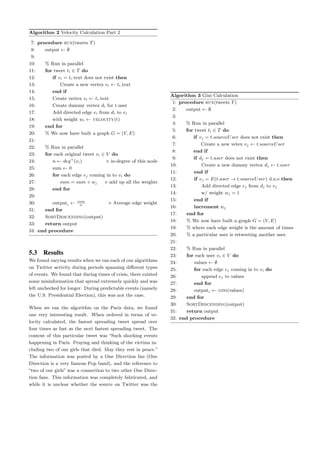
7. CONCLUSION
Temporal patterns may play a minor role in spotting vi-
tal misinformation diffusion, but if there was one conclu-
sion that we are confident about even with our limitations,
it is that there is not a direct correlation with the veloc-
ity at which information spreads and whether or not it is
misinformation. What does play a role in the velocity of
information diffusion is the popularity of the source. This
is common knowledge, but it is absolutely the case that one
with many followers will be able to spread information that
is impressive both in terms of reach and velocity. It is also
interesting that in times of confusion and chaos, it is mis-
information that travels incredibly quickly. Granted, all in-
formation is spreading at a higher rate, but misinformation
seems to spread at a disproportionately higher rate.
What does this signify? There is a chance that only in times
of crisis and turmoil is it helpful to constantly observe the
speed at which information is spreading through a network.
Fortunately, it just so happens that these are the most vital

9. times for information to be analyzed, as misinformation can
be extremely detrimental if it goes unnoticed. However, it
will hardly ever be extremely detrimental without spread-
ing. Since it is assumed that misinformation generally is
corrected succinctly and in a timely fashion, it is infeasi-
ble that information travels at a slow rate and gets a far
reach before people are able to correct and suppress it. In
other words, the measure of a snippet of information’s ve-
locity could be an extremely viable way of gauging its risk
of virality in the case that the information is actually misin-
formation. Even if this property of information diffusion is
not a clear distinction between information and misinforma-
tion, it could drastically reduce the amount of time it takes
to run more accurate misinformation detection algorithms
since the data set size can be reduced by an enormous fac-
tor if one only pays attention to the tweets with the highest
velocity, and therefore also the highest risk factor. What we
are sure of is that our algorithm(s) run extremely quickly
due to their ability to be run almost completely in parallel,
which is much more than can be said for existing misinfor-
mation detection algorithms.
8. REFERENCES
[1] A. Anagnostopoulos, R. Kumar, and M. Mahdian.
Influence and correlation in social networks. page 2,
2008.
[2] C. Castillo, M. Mendoza, and B. Poblete. Information
credibility on twitter. 2011.
[3] S. Goel, D. J. Watts, and D. G. Goldstein. The
structure of online diffusion networks. page 9, 2012.
[4] K. K. Kumar and G. Geethakumari. Detecting
misinformation in online social networks using cognitive
psychology. Human-centric Computing and Information
Sciences, pages 2–15, 2014.
[5] V. Luckerson. Fear, misinformation, and social media
complicate ebola fight. 2014.
[6] F. Vis. Hard evidence: How does false information
spread online? 2014.