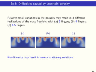
The document presents a study on numerical methods for density-driven groundwater flow, focusing on estimating the propagation of uncertainties in geo-logical parameters affecting groundwater contamination. It discusses the governing equations, stochastic modeling, and various numerical experiments conducted in both 2D and 3D reservoirs to assess the pollution dynamics and risks involved. Results indicate that uncertainties in porosity significantly affect the behavior of contaminants, and the methods developed show promise in accurately predicting groundwater quality over time.

1. Numerical methods for
density driven groundwater flow with
uncertain data
Alexander Litvinenko,
joint work with
Dmitry Logashenko, Raul Tempone, Gabriel Wittum and David Keyes
RWTH Aachen and KAUST
GAMM 2019 Conference in Vienna, Austria

2. The structure of the talk
Major Goal: estimate propagation of uncertainties in the
density-driven groundwater flow.
Plan:
1. Density-driven groundwater flow problem
2. Stochastic modeling and stochastic methods
3. Modeling of porosity
4. Numerical methods
5. 2D numerical experiments
6. 3D numerical experiments
7. Conclusion
2

3. Motivation
As groundwater is an essential nutrition
and irrigation resource, its pollution may
lead to catastrophic consequences.
(seawater intrusion into coastal aquifers,
https://water.usgs.gov/ogw/gwrp/saltwater/salt.html )
Accurate modeling of the pollution of the
soil and groundwater aquifer is difficult
due to presence of uncertainties in geo-
logical parameters.
Applications: seawater intrusion into coastal aquifers, radioactive
waste disposal, contaminant plumes etc. 3

4. What do we compute?
The mean, variance, and pdf of QoIs
Compute when dangerous concentration in a point achieve a
certain level
Forecast the pollution map in 1-5-10 years
Estimate the risk that the pollutant concentration exceeds a
certain level
4

5. Governing equations
Domain D is filled with two phases: solid porous matrix and
solution of salt in water (brine)
∂t(φρ) + · (ρq) = 0, (1)
∂t(φρc) + · (ρcq − ρD c) = 0, (2)
where c is the mass fraction of the salt, the tensor field D
represents the molecular diffusion and the mechanical dispersion of
the salt. We assume the Darcy’s law for q:
q = −
K
µ
( p − ρg), (3)
where p(t, x) is the hydrostatic pressure and g the gravity,
ρ = ρ(c) density.
5

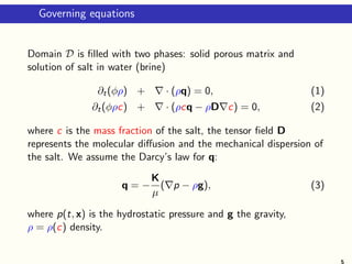
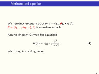
6. Governing equations
Assume permeability
K = KI, where K = K(φ) ∈ R, and I ∈ Rd×d
the identity matrix.
Use the linear dependence for the density:
ρ(c) = ρ0 + (ρ1 − ρ0)c,
where ρ0 and ρ1 denote the densities of pure water and the brine,
respectively.
Thus, c ∈ [0, 1] with c = 0 corresponding to the pure water and
c = 1 to the saturated solution.
Assume
D = φDmI,
Dm the coefficient of the molecular diffusion. We neglect the
dispersion.

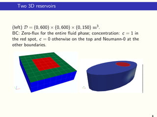
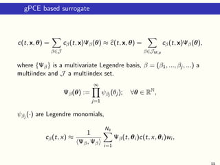
7. Computational domains
c = 1c = 0
c = 0
c = 0
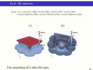
600 m
300 m
150 m
Schema of 3 layers 2D reservoir D = (0, 600) × (0, 150) and 3
realisations of the porosity.
φ(x) ∈ [0.05, 0.09], φ(x) ∈ [0.077, 0.11], and φ(x) ∈ [0.097, 0.115].
7

8. Two 3D reservoirs
(left) D = (0, 600) × (0, 600) × (0, 150) m3.
BC: Zero-flux for the entire fluid phase; concentration: c = 1 in
the red spot, c = 0 otherwise on the top and Neumann-0 at the
other boundaries.
8

9. Mathematical equation
We introduce uncertain porosity φ = φ(x, θ), x ∈ D,
θ = (θ1, ..., θM, ...), θi is a random variable.
Assume (Kozeny-Carman-like equation)
K(φ) = κKC ·
φ3
1 − φ2
, (4)
where κKC is a scaling factor.
9

10. Statistics
The empirical mean
c(t, x) ≈
Nq
i=1
wi c(t, x, θi )
def
=
Nq
i=1
wi ci ,
where Nq - number of quadrature points, wi quadrature weights, ci
are “scenarios”.
The empirical variance
Var[c](t, x) ≈
Nq
i=1
wi (c(t, x) − c(t, x, θi ))2
.
Exceedance probability (risks)
P(c > c∗
) ≈
#{c(θi ) : c(θi ) > c∗, i = 1, . . . , Ns}
Ns
.
10

11. gPCE based surrogate
c(t, x, θ) =
β∈J
cβ(t, x)Ψβ(θ) ≈ c(t, x, θ) =
β∈JM,p
cβ(t, x)Ψβ(θ),
where {Ψβ} is a multivariate Legendre basis, β = (β1, ..., βj , ...) a
multiindex and J a multiindex set.
Ψβ(θ) :=
∞
j=1
ψβj
(θj ); ∀θ ∈ RN
,
ψβj
(·) are Legendre monomials,
cβ(t, x) ≈
1
Ψβ, Ψβ
Nq
i=1
Ψβ(t, θi )c(t, x, θi )wi ,
11

12. Truncation and approximation errors
See [Constantine’12, Sinsbeck’15,Conrad’13].
Et = c(t, x, θ)−c(t, x, θ)| =
β∈Jc
cβ(t, x)Ψβ(θ), JM,p∪Jc = J .
Additionally, cβ(t, x) ≈ cβ(t, x):
Ea =
β∈JM,p
cβ(t, x)Ψβ(θ) −
β∈JM,p
cβ(t, x)Ψβ(θ)
Et+Ea =
β∈Jc
cβ(t, x)Ψβ(θ)
truncation error
+
β∈JM,p
(cβ(t, x) − cβ(t, x))Ψβ(θ)
approximation error
.
12

13. Utilized numerical methods
UG4 is a flexible software system for simulating PDE based models
on high performance parallel clusters (G. Wittum and his group).
Computation of one scenario:
1. Spatial discretization on unstructured grids.
2. Implicit Euler schema in time.
3. Newton method with line search.
4. Solution of linearized systems by BiCGStab with multigrid
preconditioning (V-cycle, ILU-smoothers).
5. Parallelisation is based on the distribution of the domain
between cores.
M scenarios are computed in parallel.
Run on 4-8 spatial grid levels with n = 0.5 . . . 8 Mio grid points.
Used 1 . . . 800 Shaheen nodes, computation time is 2-24 hours,
1000-1800 time steps, modeling time interval 5 − 8 years.
13

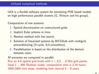
14. Ex.1: 2D example with 1 RV and small variance
φ(x, ω) = 0.09 + 0.005ξ(cos(x/300) + sin(y/150)),
where ξ ∼ U[−1, 1], in 5.5 years.
1st row: c(x) ∈ (0, 1) computed via qMC (200 simulations) and
via gPCE4 (m = 1, p = 4);
2nd row: Var[c]qMC ∈ (0, 0.021), Var[c]gPCE4 ∈ (0, 0.023).
Observed: 9 GL points gives almost the same result as 200 qMC.
14

15. Ex.2: 2D example with 2 RVs and larger variance
φ(x, ω) = 0.1 + 0.01(ξ1 cos(x/1200) + ξ2 sin(y/300)),
where ξ1, ξ2 ∼ U[−1, 1], in 1.5 years.
1st row: c(x), computed via qMC (1500 simulations) and via
gPCE, c(x) ∈ (0, 1), Var[c]qMC ∈ (0, 0.076),
2nd row: Var[c]gPCE5 ∈ (0, 0.068), Var[c]gPCE7 ∈ (0, 0.0714),
Var[c]gPCE9 ∈ (0, 0.0847).
Observed: Our surrogate and qMC give similar c.
Var[c] computed by surrogate of order 7 is most close to the qMC
variance. 15

16. Ex.3: Difficulties caused by uncertain porosity
Relative small variations in the porosity may result in 3 different
realizations of the mass fraction: with (a) 5 fingers; (b) 4 fingers;
(c) 4.5 fingers.
(a) (b) (c)
Non-linearity may result in several stationary solutions.
16

17. Ex.4: Evolution of variance in time
Below we plot Var[c] after 2.75, 5.5 and 8.25 years.
The variance is accumulated and growing.
(a) 2.75year,
Var[c](x) ∈ (0, 0.023)
(b) 5.5 year,
Var[c](x) ∈ (0, 0.055)
(c) 8.25year,
Var[c](x) ∈ (0, 0.07)
Results are obtained with 700 quasi qMC samples.
17

18. Ex.5. Elder’s problem with 5 RVs and three layers
φ(x, y, ω) =
0.08 + 0.01 5
i=1 θi sin(ixπ/600) sin(iyπ/150), 120 ≤ y ≤ 150.
0.06 + 0.01 5
i=1 θi sin(ixπ/600) sin(iyπ/150), 50 ≤ y < 120
0.09 + 0.01 5
i=1 θi sin(ixπ/600) sin(iyπ/150), 0 ≤ y < 50
(a) cgPCE; (b) cqMC in t = 5.5 years.
(c) Var[c]gPC (x, t) ∈ [0, 0.0466]; (d) Var[c]qMC (x, t) ∈ [0, 0.0556].
(e) porosity φ ∈ [0.0514, 0.09]; (f) c(x, t, 0) − c(x, t) (difference
between deterministic solution (corresponding to θ = 0) and the
mean value in t = 5.5 years,
18

19. Ex.6: 3D reservoir
φ(x, θ) = 0.1 + exp(θ1 sin(πx/600) + θ2 sin(πy/600) + θ3 sin(πz/150) + θ1 sin(πx/600)+
+ θ1 sin(πx/600) sin(πy/600) + θ2 sin(πx/600) sin(πz/150) + θ3 sin(πy/600) sin(πz/150)).
(a) (b)
Five isosurfaces of c after 9.6 years
19

20. Ex.7: Isosurfaces of Var[c] in 3D reservoir
(a) (b)
Var[c] after 4.8 years, N ≈ 8 · 106 grid points.
20

21. Ex.8: Propagation of the contamination
Evolution of the mean concentration in time after a) 0, b) 0.55, c)
1.1, d) 2.2 years. The cutting plane is (150, y, z). 21

22. Ex.9: Evolution of probability density function in a point
PDFs at aquifer point (100, 0, −25) after (a) 0.6, (b) 1.2, (c) 1.8,
and (d) 2.4 years.
22

23. Ex.10: Isosurfaces of Var[c] in 3D reservoir
(a) (b)
Isosurfaces of the variance of the mass fraction after 3 years;
(a) Var[c]0.05; (b) Var[c]0.15.
23

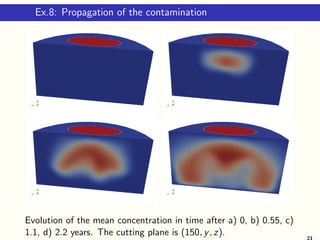
24. Ex.11: 3D reservoir with three layers
1st row: three layers of the porosity; two profiles of c;
2nd row: isosurface |cdet − c|0.25; isosurfaces Var[c]0.05 and
Var[c]0.12.
24

25. Conclusion
Solved time-dependent density driven flow problem with
uncertain porosity and permeability in 2D and 3D
Computed propagation of uncertainties in porosity into the
mass fraction. Computed the mean, variance, exceedance
probabilities, quantiles, risks.
Such QoIs as the number of fingers, their size, shape,
propagation time can be unstable
For moderate perturbations, our gPCE surrogate results are
similar to qMC results.
Used highly scalable solver on up to 800 computing nodes,
25

26. Acknowledgement
1. Alexander von Humboldt foundation
2. Elmar Zander (TU Braunschweig) for the sglib library.
3. KAUST, Shaheen project k1051, 2.7 Mio hours.
4. KAUST Supercomputing Lab.
5. KAUST Visualization Lab.
THANK YOU FOR YOUR ATTENTION !
26

27. Literature
1. S. Reiter, A. Vogel, I. Heppner, M. Rupp, and G. Wittum, A massively parallel geometric multigrid solver
on hierarchically distributed grids, Computing and visualization in science 16, 4 (2013), pp 151-164, DOI:
10.1007/s00791-014-0231-x
2. A. Vogel, S. Reiter, M. Rupp, A. N¨agel, and G. Wittum, UG4 – a novel flexible software system for
simulating PDE based models on high performance computers. Computing and visualization in science 16,
4 (2013), pp 165-179, DOI: 10.1007/s00791-014-0232-9
3. A. Schneider, H. Zhao, J. Wolf, D. Logashenko, S. Reiter, M. Howahr, M. Eley, M. Gelleszun, H.
Wiederhold, Modeling saltwater intrusion scenarios for a coastal aquifer at the German North Sea, E3S
Web of Conferences 54, 00031 (2018), DOI:10.1051/e3sconf/20185400031
4. P. Waehnert, W.Hackbusch, M. Espig, A. Litvinenko, H. Matthies: Efficient low-rank approximation of the
stochastic Galerkin matrix in the tensor format, Computers & Mathematics with Applications, 67 (4), pp
818-829, 2014
5. A. Litvinenko, D. Keyes, V. Khoromskaia, B. N. Khoromskij, H. G. Matthies, Tucker Tensor Analysis of
Matern Functions in Spatial Statistics, DOI: 10.1515/cmam-2018-0022, Computational Methods in
Applied Mathematics , 2018.
6. A. Litvinenko, Application of hierarchical matrices for solving multiscale problems, Ph.D. Dissertation,
Leipzig University, Germany, http://www.wire.tu-bs.de/mitarbeiter/litvinen/diss.pdf
27

28. Literature
7. S. Dolgov, B.N. Khoromskij, A. Litvinenko, H.G. Matthies, Computation of the Response Surface in the
Tensor Train data format arXiv preprint arXiv:1406.2816, 2014
8. S. Dolgov, B.N. Khoromskij, A. Litvinenko, H.G. Matthies, Polynomial Chaos Expansion of Random
Coefficients and the Solution of Stochastic Partial Differential Equations in the Tensor Train Format,
IAM/ASA J. Uncertainty Quantification 3 (1), pp 1109-1135, 2015
9. A. Litvinenko, H.G. Matthies, T.A. El-Moselhy, Sampling and low-rank tensor approximation of the
response surface, Monte Carlo and Quasi-Monte Carlo Methods 2012, pp 535-551, Springer, 2013.
10. A. Litvinenko, H.G. Matthies, Inverse problems and uncertainty quantification, arXiv:1312.5048, 2013.
11. A. Litvinenko, H.G. Matthies, Sparse data representation of random fields, PAMM: Proceedings in Applied
Mathematics and Mechanics 9 (1), pp 587-588, 2009.
28