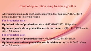
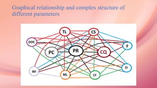
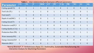
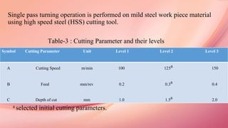
The document discusses sustainable manufacturing, focusing on optimizing parameters in the turning process to enhance productivity and minimize operational costs. It explores the influence of various machining, environmental, and economic parameters on manufacturing outcomes, utilizing graph theory and meta-heuristic algorithms, such as Taguchi and genetic algorithms, for optimization. Additionally, it presents experimental results and analyses for tool life and production rates, emphasizing the importance of cutting quality and other factors in sustainable manufacturing practices.

1. Project Guide :- Submitted by:-
Mr. Amit Kumar Sinha Sajal Dixit (2012EME05)
(Asst. Professor, DME) Senior undergraduate student
Department of Mechanical Engineering
SMVDU, J&K, India
e-mail : sajaldixit07@gmail.com

2. Sustainable Manufacturing
Manufacturing
Sustainable manufacturing
Mechanical, physical and
chemical process to modify the
geometry, properties and
appearance of a given starting
material in the making of new
finished part of product
The creation
of manufactured products that use
processes that are non-polluting,
conserve energy and natural
resources, and are economically
sound and safe for employees,
communities, and consumers.”

3. Turning Process
• A very important machining process, in which a single point cutting tool
removes unwanted material from the surface of a rotating cylindrical work
piece

4. Need of optimization and decision making in Manufacturing
Necessary for
efficient and
optimal use of
manufacturing
industries
To increase
productivity and
reduce operational
cost
Manufactures can
reduce downtime
and can increase the
value of products in
the Global market.
To increase
Quality of
Manufactured
Products

5. Parameters which effects sustainable
manufacturing in turning operation
A. Machining parameters – C. Environmental parameters-
(1) Cutting Speed (CS) (1) Water Intensity (WI)
(2) Tool Life (TL) (2) Energy Intensity (EI)
(3) Feed (F) (3) Materials (M)
(4) Depth of cut (DOC)
(5) Cutting force (CF)
B. Economical Parameters-
(1) Cutting Quality (CQ)
(2) Production Cost (PC)
(3) Production Rate (PR)

6. Graph Theory and Matrix Approach as a Decision
making Method
A graph G = (V, E) consists of a set of objects V = {v1, v2, ….} called
vertices or nodes, and another set E = {e1, e2, ….}, of which the elements
are called edges, such that each edge ek is identified with a pair of vertices.
The most common representation of a graph is by means of a diagram, in
which the vertices are represented by small points or circles, and each edge
represent the inter-relation between two end vertices.
Fig 1

7. Graphical relationship and complex structure of
different parameters

8. Table 1 . inter-relationship table between different parameters
aNeeraj Bhanota*, P. Venkateswara Raoa, S.G. Deshmukha, Sustainable Manufacturing: An
Interaction Analysis for Machining Parameters
Parameter CS TL F DOC CF PC C.Q. PR WI EI ML
Cutting speed(CS) 0 1 1 1 0 1 0 1 0 0 1
Tool Life (TL) 1 0 1 1 0 1 1 1 1 0 1
Feed rate(F) 1 0 0 0 1 1 1 1 0 0 1
Depth of cut(DOC) 1 1 0 0 1 1 1 1 0 0 0
Cutting force(CF) 1 0 1 1 0 0 0 1 0 1 1
Production cost(PC)a 1 1 1 1 1 0 1 1 0 1 1
Cutting Quality (C.Q.) 1 1 1 1 0 1 0 1 1 1 1
Production Rate (PR) 1 1 1 1 1 1 1 0 1 1 1
Water intensity(WI) 1 1 0 0 0 0 1 0 0 1 1
Energy intensity(EI)a 1 0 0 0 1 1 1 1 0 0 1
Materials (ML)a 1 1 0 0 1 1 1 1 1 1 0

9. Finding of most Influential parameters
Method :- Local Centrality Method
local centrality measure as a tradeoff between low-relevant degree centrality and
other time-consuming measures. It is a part of graph theory.
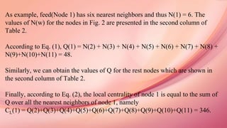
It considers nearest neighbors only. The local centrality CL(v) of node v is
defined as–
𝑄 𝑢 = 𝑤∈Γ𝑢 𝑁(𝑤) …eq.(1)
𝐶 𝐿 𝑣 = 𝑢∈𝜇(𝑣) 𝑄(𝑢) …eq.(2)
[where Γ (u) and µ(v) is the set of the nearest neighbors of node u and v
respectively . N(w) is the number of the nearest neighbor of node w.]

10. As example, feed(Node 1) has six nearest neighbors and thus N(1) = 6. The
values of N(w) for the nodes in Fig. 2 are presented in the second column of
Table 2.
According to Eq. (1), Q(1) = N(2) + N(3) + N(4) + N(5) + N(6) + N(7) + N(8) +
N(9)+N(10)+N(11) = 48.
Similarly, we can obtain the values of Q for the rest nodes which are shown in
the second column of Table 2.
Finally, according to Eq. (2), the local centrality of node 1 is equal to the sum of
Q over all the nearest neighbors of node 1, namely
CL(1) = Q(2)+Q(3)+Q(4)+Q(5)+Q(6)+Q(7)+Q(8)+Q(9)+Q(10)+Q(11) = 346.

11. S.NO PARAMETER N Q CL Contribution (%)
1 Feed (F) 6 48 346 7.98
2 Depth of Cut (DOC) 6 48 346 7.98
3 Cutting Force (CF) 6 42 319 7.36
4 Cutting Quality (CQ) 9 64 480 11.08
5 Production Cost (PC) 9 65 484 11.17
6 Production Rate (PR) 10 69 517 11.94
7 Water Intensity (WI) 5 37 277 6.39
8 Energy Intensity (EI) 6 48 346 7.98
9 Cutting Speed (CS) 6 47 348 8.03
10 Tool Life (T.L.) 8 59 437 10.09
11 Material (ML) 8 59 431 9.95
Table 2. Centrality measures for node influences

12. Meta-heuristic algorithm
• In mathematical optimization, a metaheuristic is a higher-level procedure or
algorithm which is use to provide a sufficiently good solution of an
optimization problem
• Metaheuristics are strategies that guide the search process.
• In Meta-heuristic algorithms search space is very high to find an optimum
solution that’s why it is very efficient.
• Genetic Algorithm, Ant colony algorithm (ACO), Taguchi Method are some
of the examples of Meta-heuristic procedure.

13. Optimization of Parameters
on the basis of their higher
contribution
Cutting
Quality
Product-
ion rate
Product-
ion cost
Making of
Objective
function
Design Optimization by
TAGUCHI method
Optimization by Genetic
Algorithm tool box using
MATLAB
11.08 %
11.94 %
11.17 %

14. Taguchi Method :- Optimization of Cutting Quality
• Taguchi method is a powerful tool for the design of high quality system.
• It provides a system efficient and systematic approach to optimize designs for
performance, quality and cost.
• Here we are using Taguchi method to optimize cutting quality in the single pass
turning operation.
•The experimental details of using Taguchi method to determine and analyze of
optimum cutting parameter with regard to performance index such as Tool Life
which is described below.
Process Variable Response Variable
Cutting speed
Feed Tool Life
Depth of cut

15. Single pass turning operation is performed on mild steel work piece material
using high speed steel (HSS) cutting tool.
Table-3 : Cutting Parameter and their levels
a selected initial cutting parameters.
Symbol Cutting Parameter Unit Level 1 Level 2 Level 3
A Cutting Speed m/min 100 125a 150
B Feed mm/rev 0.2 0.3a 0.4
C Depth of cut mm 1.0 1.5a 2.0

16. Table 4: Experimental Layout using an L27 orthogonal array.
Experiment No. Cutting Parameter Level
A B C
Cutting speed Feed rate Depth of cut
1 1 1 1
2 1 1 2
3 1 1 3
4 1 2 1
5 1 2 2
6 1 2 3
7 1 3 1
8 1 3 2
9 1 3 3
10 2 1 1
11 2 1 2
12 2 1 3
13 2 2 1
14 2 2 2
15 2 2 3
16 2 3 1
17 2 3 2
18 2 3 3
19 3 1 1
20 3 1 2
21 3 1 3
22 3 2 1
23 3 2 2
24 3 2 3
25 3 3 1
26 3 3 2
27 3 3 3

17. Table 5: Results for Tool life and S/N ratio
S. NO. Cutting Speed(m/min) Feed(mm/rev) Depth of cut(mm) Tool life(min) S/N ratio (dB)
1. 100 0.2 1.0 758 57.60
2. 100 0.2 1.5 560 53.07
3. 100 0.2 2.0 451 50.06
4. 100 0.3 1.0 506 48.60
5. 100 0.3 1.5 372 46.78
6. 100 0.3 2.0 301 44.94
7. 100 0.4 1.0 379 44.09
8. 100 0.4 1.5 280 42.86
9. 100 0.4 2.0 225 41.45
10. 125 0.2 1.0 248 40.56
11. 125 0.2 1.5 183 39.29
12. 125 0.2 2.0 147 37.85
13. 125 0.3 1.0 166 36.98
14. 125 0.3 1.5 122 35.73
15. 125 0.3 2.0 99 34.33
16. 125 0.4 1.0 125 33.03
17. 125 0.4 1.5 92 32.10
18. 125 0.4 2.0 74 30.97
19. 150 0.2 1.0 100 30.46
20. 150 0.2 1.5 73 29.64
21. 150 0.2 2.0 59 28.60
22. 150 0.3 1.0 67 27.90
23. 150 0.3 1.5 49 26.90
24. 150 0.3 2.0 40 25.78
25. 150 0.4 1.0 49 24.34
26. 150 0.4 1.5 37 23.55
27. 150 0.4 2.0 30 22.58

18. SYMBOL PARAMETER Mean S/N Ratio
Level 1 Level 2 Level 3 Max.-Min.
A Cutting Speed 47.71 35.68 26.65 21.05
B feed 40.79 36.45 32.81 7.98
C Depth of Cut 38.18 36.69 35.17 3.005
Total Mean S/N Ratio = 36.68 dB
Table 6 : S/N response table for tool life
Extended Taylor tool life Equation :-
𝑉𝑇 𝑛 𝑓 𝑎 𝑑 𝑏 = 𝐶
n = 0.20 C = 273 for Mild Steel work piece material
a = 0.20 - For HSS tool material
b = 0.15
Optimal Cutting Parameter – A1B1C1

19. SYMBOL Cutting
Parameter
Degree of
freedom
Sum of
Squares
Mean
Square
Contribution(%)
A Cutting Speed 2 669.78 334.89 85.88%
B Feed rate 2 95.76 47.88 12.27%
C Depth of cut 2 14.34 7.17 1.83%
Table 7 :Result Of the Analysis Of Variance For Tool Life
Sum of Squares
SSTR = 𝑖=1
3
𝑟𝑖(𝑒𝑖 − ē)
ri –Number of levels
ē – Mean S/N ratio of parameter
ei - S/N ratio of particular level
Mean Square deviations
MSD = SSTR/(N-1)

20. Initial Cutting
parameters
Optimal cutting
parameters
level A2B2C2 A1B1C1
S/N Ratio 36.27 42.22
Improvement in S/N
Ratio 5.95 dB
Table 8 :Result of Configuration on Experiment of Tool Life
S/N ratio – Signal to Noise ratio (λ)
Signal represent the desirable value for output characteristics and noise represent the
undesirable value for output characteristics.
It is the ratio of the mean to the standard deviation (SD).
λ = −10 log 𝑀. 𝑆. 𝐷
Here
𝑀. 𝑆. 𝐷 =
1
𝑚
⅀
1
𝑇𝑖
2
M.S.D = Mean Square Deviation
m= number of test, Ti is the value of tool life at ith test

21. Optimization of Production rate and Production cost
using Genetic algorithm
MAKING OF OBJECTIVE FUNCTION
1. Max. Production rate or min. Production time: aims to maximize number
of parts produced in a unit time interval or minimizes the time per unit part. Neglects cost
and/or profit.
.
Unit production time, t(min/pt): time to manufacture a unit of the product.
t = ts + tm+ tr(tm/T)

22. Where,
ts= setup time (min/pt); includes time needed to load/unload parts into
machine, tool setup time, etc.
tm= machining time (min/pt) .
tr= total tool replacement time (min/pt) .
T= tool life (min).
• Production rate= (1/t) = 1/ {ts+ tm+ tr(tm/T)}

23. • Unit production cost, u(Rs/pt): cost to manufacture a unit of the
product.
c = c1+ c3+ c4= kots+ kotm + [kt + kotr] (tm/T).
Where,
c1= capacity utilization cost (Rs/pt); includes machine cost, labor cost,
overhead etc.
ko= machine utilization rate (Rs/min)
c3= machining cost (associated with actual machining time); includes
cost of electricity, cutting fluids etc.
km= machining overhead (Rs/min).
c4= tool utilization cost; includes cost of cutting tool, tool re sharpening,
etc.
kt= cost per cutting edge (Rs/edge).

24. Machining time (tm)= (3.14*D*L)/(1000*v*f)
where,
D : Diameter of Workpiece(mm)
L : Length of turning(mm)
v : Cutting Speed(m/min.)
f : feed(mm/rev)
Taylor’s Tool Life Equation:
v*Tp*fq*dr = Ct
where,
T : Tool life (min.)
d: depth of cut (mm.)
Ct, p, q, r: Emperical constants

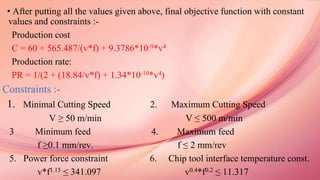
25. Objective function with constraints
1. 𝑐 = 𝑐1 + 𝑐2 ∗ 𝑣
− 1 ∗ 𝑓
− 1 + π𝐷𝐿 ∗ 𝑑
𝑟
𝑝
∗ 𝑣
1
−
𝑃
𝑝
∗
𝑓
𝑞
−
𝑝
𝑝
1000∗𝑐𝑡
1
𝑝
Where, C1 = K0*ts
C2 = π*D*L*K0/1000
2. 𝑃𝑅 = 1/{𝑡𝑠 +
𝜋𝐷𝐿
1000∗𝑣∗𝑓
+ 𝑡𝑟[(𝜋𝐷𝐿 ∗ 𝑣
1
−
𝑝
𝑝
∗ 𝑓
𝑞
−
𝑝
𝑝
∗ 𝑑
𝑟
𝑝
]/ 1000 ∗ 𝑐𝑡
1
𝑝
Following to:-
1. vmin ≤ v ≤ vmax 2. fmin ≤ f ≤ fmax
3. Pm ≥ Cn*v*d*fx 4. Qu ≥ k2*vw*fy*dz

26. Practical Data for HSS tool material for 0 degree rake angle :-
a) k0=30 Rs./min. J) K2=132
b) ts = 2 min. k) w = 0.4
c) tr = 3 min. l) y = 0.2
d) Kt = 120 Rs m) z = 0.105
e) Taylor’s Tool life constant:
i) Ct = 273
ii) p = 0.20
iii) q = 0.20
iv) r =0.15
f) D = 50 mm
g) L = 120 mm
h) d = 6 mm
i) Qu = 873 K
j) Pm = 20 KW
k) Cn =9772.3722
l) x = 1.15

27. • After putting all the values given above, final objective function with constant
values and constraints :-
Production cost
C = 60 + 565.487/(v*f) + 9.3786*10-9*v4
Production rate:
PR = 1/(2 + (18.84/v*f) + 1.34*10-10*v4)
Constraints :-
1. Minimal Cutting Speed 2. Maximum Cutting Speed
V ≥ 50 m/min V ≤ 500 m/min
3 Minimum feed 4. Maximum feed
f ≥0.1 mm/rev. f ≤ 2 mm/rev
5. Power force constraint 6. Chip tool interface temperature const.
v*f1.15 ≤ 341.097 v0.4*f0.2 ≤ 11.317

28. Solution of objective function by genetic algorithm tool box using MATLAB
Code for the Maximization of Production Rate:
function P = production_rate(x)
P = -(1/(2+18.84/(x(1)*x(2))+1.34*10^-10*x(1)^4.0));
end
Code for the Minimization of Production Cost:
function C = Production_cost(x)
C = 60+565.487/(x(1)*x(2))+9.3786*10^-9*x(1)^4.0;
end

29. Code for the Inequality Constraints:
function [T, ceq] = nonlinear_constraints(x)
T = [x(1)*x(2)^1.15-341.097;
x(1)^0.4*x(2)^0.2-11.317];
ceq = [];
end
[The above code will be applied on both the basic optimization function]
Main code to find Optimum points for Production rate and Production cost
ObjFcn = @production_rate/@production_cost;
nvars = 2;
LB = [50,0.1];
UB = [500,2.0];
ConsFcn = @nonlinear_constraints
[x, fval] = ga(ObjFcn, nvars, [], [], [], [], LB, UB, ConsFcn);

30. Result of optimization using Genetic algorithm
After running main code and Genetic algorithm tool box in MATLAB for 5
iterations, it gives following result :
For Production rate –
Optimized value of production rate = 0.4750160018531908 pt/time
Optimum points where production rate is maximum : x(1)= 111.9379 m/min,
x(2)= 2.0 mm/rev
For Production cost –
Optimized value of production cost = 63.739932123648494 Rs./pt
Optimum points where production cost is minimum : x(1)= 94.5015 m/min,
x(2)= 2.0 mm/rev

31. Screen-shots of Genetic algorithm tool box and main code in MATLAB