The document covers structural modeling in Verilog, emphasizing its advantages over dataflow modeling and outlining the essential components like primitives, delays, and synthesis directives. Key topics include the importance of hand-designed systems, the use of hierarchical designs for adders, and component instantiation methods. It concludes by highlighting how structural modeling serves as a foundational approach for designing efficient digital systems using Verilog.

1. 1
Structural Modeling
Vasudeva Murthy T

2. 2
Session Objectives
• To understand the importance and advantages of
structural modeling
• To learn about the different primitives in the language
• To understand the usage of delays in simulation
• To create an awareness of synthesis and compiler
directives
• To comprehend the relevance of various forms of
instantiation
• To learn to make a code scalable

3. 3
Session Topics
• Disadvantages of dataflow modeling
• Verilog in-built primitives
• Delay operators and their usage
• Synthesis and compiler directives
• Reference by name/ position
• Parameters
• Generate block

4. 4
Cons of Dataflow Modeling
• Almost all present day problems have solutions in the
form of FSMs
• Purely combinational circuits rarely required
• Dataflow can not model sequential logic
• Continuous assignment statements always active –
sometime unnecessarily
• Designer might not have complete control over hardware
generated

5. 5
Necessity of structural modeling
• Hand-Designed systems always the most efficient
• Power, area, frequency requirement can be most
accurately met by designer
• Existence of proven sub-blocks
• IP-Cores readily available
• Existing functional system requires minute tweaking

6. 6
Structural Modeling
• Structural modeling:
– Involves building of design using pre-defined gates
– Smaller sub-modules are instantiated
– Can be considered as schematic in text form
• Primitives
– Pre-defined gates already described in the Verilog language
– Can have only one output but any number of inputs
– Language has no restriction on inputs but depends on
technology being targeted to
– All basic combinational gates available as primitives
– Used directly in the code as smaller case key-words
– and, nand, or, nor, not, xor, xnor, buf, bufif1, bufif0

7. 7
Using Primitives
module mux(
output z,
input I0, I1, sel);
not #(1.1, 1) Inv (nsel, sel);
and #(1.8,1.5) A0(a0, nsel, I0),
A1(a1,sel,I1);
or #(1.8, 1.6) O(z,a1,a2);
endmodule
• First variable in port list of primitive is always output
• Naming of primitives is optional
A1
A0
O
Inv
nSel
a1
a0

8. 8
Timescale directive
`timescale 1 ns/ 10ps
module adder(
output sum, carry,
input a,b,cin);
xor #(2.1, 2) XO (sum,a,b,cin);
and #1.8 A0(a0, a,b),
A1(a1,b,cin),
A2(a2,cin,a);
or #(1.8, 1.605) O(carry,a0,a1,a2);
endmodule
And gate has equal rise time and fall time
of 1.8 ns
`timescale :
•Defines the time units to be used
•Wherever the delay operator is
encountered the time units will be
considered as 1 ns
•The delay can be upto a precision of 10
ps
•Here xor gate which has name ‘XO’
has a rise time of 2.1 ns and a fall time
of 2 ns
•or gate which has name ‘O’ has rise
time of 1.8 ns and fall time of 1.6 ns.
•The 1.605 will be rounded of to 1.600
as 0.005 is lesser than precision 10 ps
specified

9. 9
Compiler directive
`timescale 1 ns/ 10ps
`default_nettype none
module mux(
output wire z,
input wire I0, I1, sel);
wire nsel, a0, a1;
not #(1.1, 1) Inv (nsel, sel);
and #(1.8,1.5) A0(a0,
nsel, I0),
A1(a1,sel,I1);
or #(1.8, 1.605)
O(z,a1,a2);
endmodule
`default_nettype :
•Value none specifies that
undefined variables should not
default to type wires
•Simulator requires even port’s
data type to be declared , hence
‘z,I0,I1,sel’ also declared as
wires
•Synthesis tool requires only
internal wires ‘nsel, a0, a1’ to be
explicitly declared
•Forces the designer to declare all
internal wires
•Any variable starting with ` is a
compiler directive

10. 10
Primitives explained
module adder(
output sum, carry,
input a,b,cin);
xor #(2.1, 2) XO (sum,a,b,cin);
and #1.8 A0(a0, a,b),
A1(a1,b,cin),
A2(a2,cin,a);
or #(1.8, 1.605) O(carry,a0,a1,a2);
endmodule
Primitives
•In-built gates which are
instantiated
•They need not be declared, they
are only called
•First variable is understood to be
output
– Here sum, a0,a1,a2, carry are
outputs of ‘xor’, ‘and’ gate A0,
‘and’ gate A1, ‘and’ gate A2,
and ‘or’ gate respectively
•They can be optionally named
•Delays can be specified - again
optionally
• Any number of gates of same
functionality can be called in
single line
– Here three and gates A0,A1 and
A2 are being called in same line

11. 11
Component Instantiation
• Instantiation
– Predefined modules can be called just like primitives
– An Instance is a unique copy of a pre-defined module
– Connected to one another by means of nets
A
B
Cin
Sum
Carry

12. 12
Component Instantiation Example
`timescale 1ns/10ps
module adder(
output sum, carry,
input A, B, Cin);
wire axorb, nB, nCin;
not #(1.1, 1) (nB,B), (nCin,Cin);
mux XOR (axorb, B, nB, A); // improper way of instantiating
mux SUM (.Z(sum), .I0(Cin), .I1(nCin), .sel(axorb)),
CARRY (.Z(carry), .I0(A), .I1(Cin), .sel(axorb));
endmodule

13. 13
Component instantiation rules
• Component instantiation can be done in two ways
– Named port connection / calling by reference
• Mostly preferred in the Industry
– Ordered port connection / calling by position
• An error prone way of instantiating
• Most simulators / synthesis tools require components to
be compulsorily named
• Component can be called more than once in a single line
• Component instantiations do not accommodate delays like
primitives
• While simulating component should have been compiled
before it can be called in a top module

14. 14
Component Instantiation explained
not #(1.1, 1) (nB,B), (nCin,Cin);
mux XOR (axorb, B, nB, A);
mux SUM (.Z(sum), .I0(Cin), .I1(nCin), .sel(axorb)),
CARRY (.Z(carry), .I0(A), .I1(Cin), .sel(axorb));
endmodule
primitives do not require names,
components do require
primitives can have delays,
components can not have delays
components can be referenced
by ordered port connection

15. 15
Component Instantiation explained
• mux XOR (axorb, B, nB, A); // module mux(output z,input I0, I1, sel);
– In Multiplexer ‘XOR’ port axorb refers to port Z of original ‘mux’
– Similarly port B and port nB are connected to I0 and I1 of ‘mux’
– While port A is connected to port ‘sel’ of reference design ‘mux’
– These connections are order dependent
• Components are preferred to be connected by name
• The names of the reference design ports are associated with DOT
• The names of the connections in the module is written in brackets
mux SUM (.Z(sum), .I0(Cin), .I1(nCin), .sel(axorb)),
CARRY (.Z(carry), .I0(A), .I1(Cin), .sel(axorb));
• In the above example the original design ports are being referred by name
• The interconnects of the sub-modules are being passed through brackets

16. 16
• An adder built of many single bit adders
• Has three inputs, two of which are buses
• Has two outputs one of which is a bus
Hierarchal Design
sum
carry
_out
B Co
Su
Ci
A
B Co
Su
Ci
A
B Co
Su
Ci
A
first
second
carry
_in

17. 17
A 4-bit ripple-carry adder
• Four full adders together make a 4-bit adder.
• There are nine total inputs:
– Two 4-bit numbers, A3 A2 A1 A0 and B3 B2 B1 B0
– An initial carry in, CI
• The five outputs are:
– A 4-bit sum, S3 S2 S1 S0
– A carry out, CO
• Imagine designing a nine-input adder without this hierarchical
structure—you’d have a 512-row truth table with five outputs!

18. 18
Hierarchical adder design
• When you add two 4-bit numbers the carry in is always 0, so why does the
4-bit adder have a CI input?
• One reason is so we can put 4-bit adders together to make even larger
adders! This is just like how we put four full adders together to make the 4-
bit adder in the first place.
• Here is an 8-bit adder, for example.
CI is also useful for subtraction.

19. 19
A two’s complement subtraction circuit
• To find A - B with an adder, we’ll need to:
– Complement each bit of B.
– Set the adder’s carry in to 1.
• The net result is A + B’ + 1, where B’ + 1 is the two’s complement
negation of B.

20. 20
Small differences
The only differences between the adder and subtractor circuits are:
– The subtractor has to negate B3 B2 B1 B0.
– The subtractor sets the initial carry in to 1, instead of 0.
It’s not too hard to make one circuit that does both addition and
subtraction.

21. 21
Adders/Subractors
• XOR gates let us selectively complement the B input.
• X  0 = X X  1 = X’
• When Sub = 0, the XOR gates output B3 B2 B1 B0 and the carry in is 0. The adder
output will be A + B + 0, or just A + B.
• When Sub = 1, the XOR gates output B3’ B2’ B1’ B0’ and the carry in is 1. Thus,
the adder output will be a two’s complement subtraction, A - B.

22. 22
N Bit adder
• Consists of various single bit adders
• Has two multi-bit inputs
• Output is also multi-bit
• All adders except the first and last are similar in nature
• Adder circuit having ‘n’ adders will have n+1 wires to
transport carry signals

23. 23
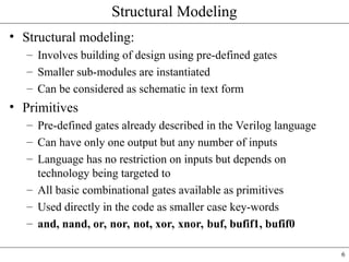
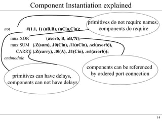
Code for hierarchal design
1. module adder_bit_n #(parameter n = 8)
2. (output [n-1:0] sum,
3. output carry_out,
4. input [n-1:0] first, second,
5. input carry_in);
6. genvar j;
7. wire [n:0] carry_wires;
8. assign carry_wires[0] = carry_in;
9. generate
10. for(j=0; j <n; j = j+1)
11. begin :series
12. adder
A(.A(first[j]), .Ci(carry_wires[j]), .B(second[j]), .Su(sum[j]), .Co(carry_wires[j+1]));
13. end
14. endgenerate
15. assign carry_out = carry_wires[n];
16. endmodule

24. 24
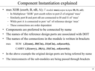
Vectors
• Signals which are multi-bits are declared as vectors
• Can be declared as [high:low] or [low:high]
• The left hand value always specifies the index of the MSB
• A bit of the vector is accessible
• Example
– see previous example
• wire [n:0] carry_wires // line 7 – vector being declared
• carry_wires[0] =carry_in // line 8 – Bit of vector is assigned
• carry_out = carry_wires[n] // line 15 – Bit of vector is accessed
• carry_wires[5:2] = 4’d1010 // part of vector being assigned value
• outp = carry_wires[n-1:n-5] // part of vector being accessed

25. 25
Parameters
• Parameters are run time constants
• Are declared within a module
• Their scope lies within the module
• Can be overwritten using “defparam”
• Can be overwritten during component instantiation
• Used to make a code scalable
• Module can have more than one parameter
• Example
– In the previous example ‘n’ is a parameter with value ‘8’

26. 26
Generate Statement
Generate:
• As the name specifies used to generate a set of hardware
• Simply replicates a given set of function for a specified number of
times
• Two generate statements available
– for generate
• Variables used inside for generate loop known as ‘genvar’
– genvar j // line 6 – j is a variable used in for loop in previous example
• Loop inside for generate should be labeled
– begin : series // line 11 – for loop labeled with name ‘series’
– if generate
• Used for conditional use of hardware / logic
• Statement is concurrent in nature

27. 27
Summary
• Hand-Designed systems always the most efficient
• Structural elements of a Verilog structural description are logic
gates and user-defined components connected by wires
• Structural description can be viewed as a simple netlist composed
of nets that connect instantiations of gates
• Primitives have been identified as basic building blocks of
structural modeling, their types and usage has been understood
• Compiler directives have been found to make coding effort easier
• Component instantiation statements and their operation has been
studied
• Generate blocks are used to replicate most commonly used
hardware Verilog structural modeling has been discussed
• Run time constants and generate blocks have been discussed