Stock market prediction employing ensemble methods: the Nifty50 index

IAES International Journal of Artificial Intelligence (IJ-AI)
Vol. 13, No. 2, June 2024, pp. 2049~2059
ISSN: 2252-8938, DOI: 10.11591/ijai.v13.i2.pp2049-2059  2049
Journal homepage: http://ijai.iaescore.com
Stock market prediction employing ensemble methods: the
Nifty50 index
Chinthakunta Manjunath1
, Balamurugan Marimuthu1
, Bikramaditya Ghosh2
1
Department of Computer Science and Engineering, School of Engineering and Technology, Christ University, Bengaluru, India
2
Symbiosis Institute of Business Management, Symbiosis International (Deemed University), Bengaluru, India
Article Info ABSTRACT
Article history:
Received Aug 1, 2023
Revised Nov 15, 2023
Accepted Dec 3, 2023
Accurately forecasting stock fluctuations can yield high investment returns
while minimizing risk. However, market volatility makes these projections
unlikely. As a result, stock market data analysis is significant for research.
Analysts and researchers have developed various stock price prediction
systems to help investors make informed judgments. Extensive studies show
that machine learning can anticipate markets by examining stock data. This
article proposed and evaluated different ensemble learning techniques such
as max voting, bagging, boosting, and stacking to forecast the Nifty50 index
efficiently. In addition, an embedded feature selection is performed to
choose an optimal set of fundamental indicators as input to the model, and
extensive hyperparameter tuning is applied using grid search to each base
regressor to enhance performance. Our findings suggest the bagging and
stacking ensemble models with random forest (RF) feature selection offer
lower error rates. The bagging and stacking regressor model 2 outperformed
all other models with the lowest root mean square error (RMSE) of 0.0084
and 0.0085, respectively, showing a better fit of ensemble regressors.
Finally, the findings show that machine learning algorithms can help
fundamental analyses make stock investment decisions.
Keywords:
Bagging
Boosting
Fundamental analysis
Machine learning
National stock exchange fifty
Stacking
Stock market forecasting
This is an open access article under the CC BY-SA license.
Corresponding Author:
Chinthakunta Manjunath
Department of Computer Science and Engineering, School of Engineering and Technology
Christ University
Mysore Road, Kengeri Campus, Kumbalgodu, Bengaluru, India
Email: manju.chintell@gmail.com
1. INTRODUCTION
In the field of financial economics, a crucial topic is the connection that exists between the
performance of markets and the risk that is associated with the economy. According to the broadly
recognized random walk theory (RWT), the markets operate randomly and unexpectedly [1], [2]. The prompt
and precise reflection of all available information in the prices of securities characterizes an efficient market
hypothesis (EMH). Market efficiency is categorized into three distinct forms: weak, semi-strong, and strong
forms. They claim that technical or fundamental analysis cannot forecast stock prices [3]. Fundamental and
technical stock investment analyses increase investor decision-making and profitability. Many astute
investors employ diverse approaches, such as fundamental and technical analysis, forecasting algorithms, and
functions to forecast equity prices and their performance [4]. The first supports long-term forecasting and
requires a detailed review of a firm’s economic status, monetary environment, liabilities, leadership, assets,
goods, and competition [5], [6], while the latter forecasts stock price trends based on past changes and used
for short-term forecasting [7]. However, the fractal market hypothesis (FMH)-proposes that financial markets
exhibit fractal patterns and self-similarity across different timeframes. FMH considers the daily randomness

 ISSN: 2252-8938
Int J Artif Intell, Vol. 13, No. 2, June 2024: 2049-2059
2050
of the market, and prices can be predicted with market characteristics such as non-linearity and long-term
dependence [8]. Empirical evidence shows stock prices do not follow random walks [9]. According to
modern behavioral finance experts, investors are emotional, and their cognitive biases driven by external
market sentiments affect firm value and stock price [10]–[12]. Stock values have been evaluated since the
market’s creation, and retail participation in Indian stock markets has increased significantly. As India’s
economy rises, it is stock market will improve, attracting capital and investors. There are many kinds of
research works in forecasting using time series analysis. The fundamental analysis benefits long-term
investors, but day traders ignore it. Thus, fundamental analysis is vital to making long-term stock investment
selections. Some of the most significant tasks based on this are listed here.
The stock market’s performance affects other macroeconomic parameters and determines an
economy’s direction. For instance, Tripathi and Seth [13] used macro variables, such as currency, interest,
and inflation rates, affecting the Nifty50 market. A country’s stock market maturity, currency value, and
interest rate reveal its traits [14]. Mishra and Dhole [15] examined the national stock exchange (NSE) stock
co-movement. Synchronization is negatively connected with business group association and leverage and is
positively correlated with growth and profit volatility. To assess the long-term relationship between Indian
equities market value and macroeconomic variables (exchange rate, foreign reserve, and consumer price
index (CPI)), Yadav et al. [16] used vector error correction model (VECM) and Johansen’s co-integration
tests. Currency exchange rates have long intrigued economists, policymakers, and investors [17]. Economic
dynamics and market performance are strongly correlated, as shown by several research. The connection
between the stock market and its stock market returns in Pakistan, India, China, South Korea, and Hong
Kong is examined. This analysis yields two key conclusions. First, there are options for investor
diversification; second, domestic factors (macroeconomic variables) impact stock markets [18].
Autoregressive moving average (ARMA) and macroeconomic factors were used to analyze bombay stock
exchange (BSE) returns. The analysis found that foreign institutional investments (FIIN), risk in standard and
poor’s (RS&P), standard and poor’s (S&P) 500 return, and United States treasury bill rate (USTBR) had
large and positive regression coefficient values, showing that these four factors positively impact the Indian
stock market [19]. An event study approach was analyzed on samples of Russian and Indian businesses.
Berezinets et al. [20] conclude that both good and poor dividend surprises cause the Russian market to react
negatively; good dividend surprises cause optimistic irregular earnings on Indian equities, while wicked and
no astonishments cause undesirable reactions in the Indian market. In addition, Misra [21] examined the
association between macroeconomic factors and the BSE SENSEX. All the variables exhibit long-run
causation, while only inflation and the money supply exhibit short-run causality. Patel [22] found the BSE
and S&P CNX Nifty were affected by the exchange rate, index of industrial production (IIP), inflation,
money supply, silver, oil, and gold prices. The unit root was found using the augmented dickey-fuller test
(ADF), Johansen co-integration test, VECM, and Granger causality tests.
Additionally, he found a connection between the exchange rate, oil prices, IIP, and stock market
indices. Finally, Gopinathan and Durai [23] found long-term correlations between fundamental factors.
VECM tests, Johansen co-integration, and summary statistics examine fluctuations. Additional
macroeconomic issues that may affect the stock market would expand the study. AI incorporates machine
learning. Some stock prediction studies included fundamental analysis and machine learning. Quah [24]
compared three basic stock selection machine learning algorithms. Graham’s book encouraged this author to
forecast 11 popular financial ratios [25]. Macro and microeconomic factors affect investment outcomes.
Random forest (RF) outperformed support vector machine (SVM) and naive Bayes (NB) with 0.751 F-score
to predict stocks using eleven fundamental metrics [26]. The research examines whether fractal patterns are
present in the behavior of the EURIBOR panel banks across multiple Eurozone nations [27].
From the literature, fundamental analysis predicts, performs, and analyzes market price movements
using micro and macroeconomic data. A few aspects must be considered to develop a more useful predictive
model utilizing this approach: i) the earlier study featured multi-collinearity and correlated input factors;
ii) endogeneity can bias the estimates and mislead; iii) financial time series are non-stationary, non-linear,
high-noise, and may not reflect complicated dynamics, making traditional statistical models challenging to
predict; and iv) the literature review showed various feature selection methodologies essential for
constructing reliable prediction algorithms. This study adds the following to scientific understanding to fill
the research gaps in previous studies: i) this study uses state-of-the-art ensemble learning algorithms to
capture the financial market’s complex non-linear patterns, and dynamics by employing a fundamental
analysis-based approach; ii) this work contributes by selecting highly perceptive features from an existing
collection of fundamental characteristics using an embedded feature selection strategy to improve model
performance with fewer features; iii) the GridSearchCV technique has been utilized to determine the optimal
hyperparameter to enhance the model’s performance; and iv) the results showed that bagging and stacking
ensemble models using RF feature selection had the lowest error rates.

Int J Artif Intell ISSN: 2252-8938 
Stock market prediction employing ensemble methods: the Nifty50 index (Chinthakunta Manjunath)
2051
2. METHOD
2.1. Data preparation and pre-processing
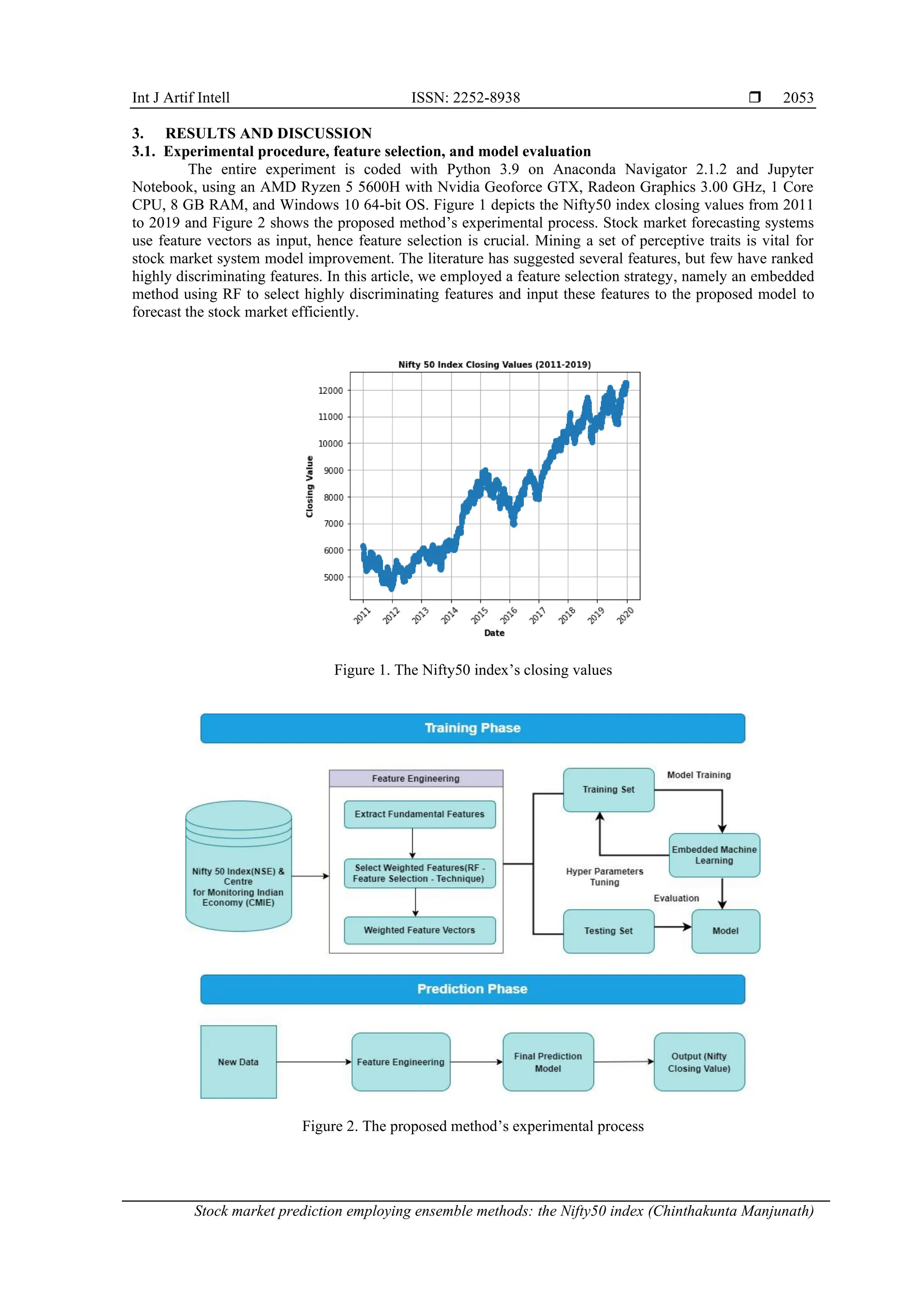
The prediction in this work is based on a fundamental analysis approach. In this experiment,
fundamental indicators for the period Jan 2011 to Dec 2019 were obtained from the Reserve Bank of India
and NSE databases. Table 1 depicts the fundamental indicators and its description. All these fundamental
indicators forming feature set of the proposed ensemble regressors and analysis of the Indian stock market on
the Nifty50 index. Prior to further processing, these characteristics were normalized to the interval [0, 1].
However certain traits may be unnecessary and provide information that is already known for the learning
task, while others may be useful and provide false information that impairs learning outcomes. In this work, a
feature selection strategy based on embedded systems is adopted to eliminate features that are unnecessary or
redundant. Feature selection is integrated into the classifier via an embedded approach. The advantages of both
filter and wrapper methods are combined in embedded methods, which represent a hybrid approach [28], [29].
Table 1. Fundamental indicators used
Feature name Description of the feature
Price-to-earnings (P/E) ratio The P/E ratio quantifies the relative valuation of a company’s shares in
relation to it is earnings per share (EPS).
Price-to-book (P/B) ratio How much an investor is willing to pay for a firm compared to its book
value is what the P/B ratio reveals.
Dividend yield Dividend yield measures annual dividend payout as a percentage of stock
price and is a standard financial indicator of a company’s financial health.
Exchange rate The term “exchange rate” refers to the agreed-upon percentage by which
one currency can be traded for another in the financial market. This study
considers the US Dollar, Pound Sterling, Euro, and Japanese Yen exchange
rates.
Inflation (CPI and WPI) The rate at which inflation causes prices across the board to rise is known
as the inflation rate.
Gross domestic product (GDP) It estimates a country’s GDP and growth rate by providing an economic
snapshot.
Index of industrial production (IIP) The IIP measures the health of India’s manufacturing sector. There are
three main categories within IIP: industry, mining, and energy production.
2.2. Base model: support vector regressor
Supervised machine learning reduces error and increases geometric margins with the SVM. It is a
regression and pattern categorization algorithm. SVM mapped non-linear samples to a large-dimensional
space using a kernel function, making them linearly separable. Different kernel functions greatly affected
SVM classification performance. The radial basis function (RBF) was frequently employed in practical
applications due to it is fewer parameters and superior performance [30], [31]. The RBF kernel formula is:
𝐾( 𝑥, 𝑥𝑖) = exp ( −
||𝑥−𝑥𝑖 ||2|
𝜎2 )
where x and xi are ample vectors, δ is the RBF kernel function and a free parameter.
2.3. Ensemble techniques
Meta-algorithms called “ensemble approaches” blend multiple machine learning methods into one
forecasting model to either reduce variance (bagging) or bias (boosting) or to improve forecasts. It also
enhances robustness and provides a generalized model [32]. This article discusses the fundamental analysis
of stock market forecasting utilizing ensemble approaches, including max-voting, bagging, boosting, and
stacking. Max voting is typically applied to classification or regression problems. Each model predicts and
votes for each sample. The prediction class contains only the sample class’s highest-voted class. Bootstrap
aggregation, often known as bagging classifier/regressor, is an early ensemble method intended to reduce
variance. They aggregate predictions from each regressor model trained on a random subset of the training
data. The RF method is efficient at feature selection. RF is a reliable strategy for dealing with imbalanced,
missing, and multicollinear data. Algorithm 1 shows the bagging steps. Boosting is an ensemble learning
method that strengthens weak learners to reduce training errors. AdaBoost is an ensemble learning method
that stands for adaptive boosting, and in this method, weak learners are helped by increasing their weights
and allowing them to vote on the final model. AdaBoost regressor fits the dataset and adjusts weights based
on the error rate. Algorithm 1 is an illustration of the method. Algorithm 2 shows the AdaBoost technique.

 ISSN: 2252-8938
2052
Algorithm 1: Bagging
Input:
Dataset 𝑆 = {𝑥𝑖𝑦𝑖} 𝑛
𝑖=1
; Base learning algorithm 𝐿; Several base learners 𝑚.
Process:
𝑓𝑜𝑟 𝑗 = 1 𝑡𝑜 𝑚:
𝑆𝑗 = 𝑏𝑜𝑜𝑡𝑠𝑡𝑟𝑎𝑝(𝑆); // Generate a bootstrap sample from S
ℎ𝑗 = 𝐿(𝑆𝑗) // From the bootstrap sample, train a base learner ℎ𝑗
end.
Output:𝐻(𝑥) = 𝑚𝑜𝑑𝑒𝑙( ℎ1(𝑥), … . , ℎ𝑚(𝑥))
Algorithm 2: AdaBoost technique
Input: Dataset = {𝑥𝑖𝑦𝑖} 𝑚
𝑖=1
. A weight vector 𝑍𝑡 is created based on the weight of each training set sample;
The number of learning rounds is given by T, while L stands for the fundamental learning algorithm.
Process:
Step 1: Initializing the weight distribution
𝐷1(𝑖) = 1
𝑚
⁄
Step 2: for 𝑡 = 1,2, … . , 𝑇:
ℎ𝑡 = 𝐿 {𝐷, 𝐷𝑡}; //Using distribution, 𝐷𝑡 train a base learner ℎ𝑡 from 𝐷.
𝜖𝑡 = 𝑃𝑟𝑖~𝐷1
[ℎ𝑡(𝑥𝑖 + 𝑦𝑖 )]; // Calculate the error of ℎ𝑡
𝛼𝑡 =
1
2
𝑙𝑛
1−𝜖𝑡
𝜖𝑡
// The distribution update using 𝑧𝑡 a normalization factor that enables 𝐷𝑡+1to be a distribution
𝐷𝑡+1(𝑖) =
𝐷𝑡(𝑖)
𝑠𝑢𝑚(𝑍𝑡)
×{
exp (−𝛼𝑡) 𝑖𝑓 ℎ𝑡(𝑥𝑖) = 𝑦𝑖
exp (𝛼𝑡) 𝑖𝑓 ℎ𝑡(𝑥𝑖) ≠ 𝑦𝑖
end
Output: 𝐹(𝑥) = 𝑠𝑖𝑔𝑛 ∑ 𝑎𝑡
𝑇
𝑡=1 ℎ𝑡(𝑥)
Stacking is an ensemble learning approach aggregating results from many classifications or
regression models using a meta-classifier or meta-regressor. A series of learning algorithms form the stacking
ensemble’s base, making it very diversified. The stacking ensemble technique considered the primary
classifier and meta classifier’s learning capabilities, improving the final classification’s performance [33]. In
this proposed stacking, the outputs of the models are combined to obtain the final prediction for any
instance 𝑥𝑖. Stacking introduces a level-1 approach called meta-learner to learn the weights 𝛽𝑗 of the level-0
predictors. That is, for the meta learner (level-1), the prediction 𝑦(𝑥𝑖) of each training instance 𝑥𝑖 is training
data, which can be described as follows:
𝑦(𝑥𝑖) = ∑ 𝛽𝑗
4
𝑗=1 ℎ𝑗( 𝑥𝑖)
where 𝑥𝑖 is the samples, 𝛽𝑗 is the optimal weight of level-0 predictors, and ℎ𝑗 is the base model. The stacking
algorithm is discussed briefly in Algorithm 3.
Algorithm 3: Stacking ensemble
Input: Dataset 𝐷 = {𝑥𝑖𝑦𝑖} 𝑚
𝑖=1
Process:
Step 1: learning regressors at the first level
for 𝑡 = 1 𝑡𝑜 𝑇 do
Learn a 𝑟𝑡 base learning algorithm based on D
end for
Step 2: Build a novel dataset of forecasts from D
for 𝑖 = 1 𝑡𝑜 𝑚 do
𝐷ℎ = { 𝑥𝑖
′
𝑦𝑖}, where 𝑥𝑖
′
= { ℎ1(𝑥𝑖), … . , ℎ𝑇(𝑥𝑖)}
end for
Step 3: A meta-learning regressor: Learn 𝑅 based on 𝐷ℎ
return R
Output: R: An ensemble regressor.

2053
3. RESULTS AND DISCUSSION
3.1. Experimental procedure, feature selection, and model evaluation
The entire experiment is coded with Python 3.9 on Anaconda Navigator 2.1.2 and Jupyter
Notebook, using an AMD Ryzen 5 5600H with Nvidia Geoforce GTX, Radeon Graphics 3.00 GHz, 1 Core
CPU, 8 GB RAM, and Windows 10 64-bit OS. Figure 1 depicts the Nifty50 index closing values from 2011
to 2019 and Figure 2 shows the proposed method’s experimental process. Stock market forecasting systems
use feature vectors as input, hence feature selection is crucial. Mining a set of perceptive traits is vital for
stock market system model improvement. The literature has suggested several features, but few have ranked
highly discriminating features. In this article, we employed a feature selection strategy, namely an embedded
method using RF to select highly discriminating features and input these features to the proposed model to
forecast the stock market efficiently.
Figure 1. The Nifty50 index’s closing values
Figure 2. The proposed method’s experimental process

 ISSN: 2252-8938
2054
Table 2 provides information on different feature selection techniques, the corresponding feature
selection algorithms used, the selected feature sets, and the number of features used for each method. These
were then chosen for model development and conducting experiment results. Table 3 provides an overview
of the base and ensemble models used in the proposed work. These models leverage different techniques to
enhance prediction accuracy and capture the relationships between the features and the target variable.
Table 2. Feature selection type and its algorithm
Feature selection type Feature selection algorithm Feature set Number of features used
Embedded Random forest {Euro, US_Dollar, Pound_Sterling, P_E,
Japanese_Yen, P_B, Div_Yield}
7
Table 3. Proposed work’s base and ensemble models
Models Base and ensemble techniques
Support vector regression (SVR) Base regressor
MAX Voting Ensemble voting regressor
Bagging with RF Ensemble bagging regressor
Boosting with AdaBoost Ensemble boosting regressor
Stacked regressor model 1 Base learners-RF, gradient boosting regression (GBR), and SVR. Final estimator-linear
regression (LR).
Stacked regressor model 2 Base learners-decision tree regressor (DTR), GBR, and SVR. Final estimator-RF
Machine learning tasks are associated with evaluation metrics, and because we are attempting to
forecast future stock values using machine learning methodologies, we must employ many evaluation metrics
to assess and determine our model’s performance and behavior. As demonstrated in (1)-(4), mean square
error (MSE), root mean square error (RMSE), mean absolute percentage (MAP), and coefficient of multiple
determinations for multiple regressions (𝑅2
) were utilized to evaluate the efficacy of our suggested
approaches. These criteria are preferred to be smaller because they represent the models’ prediction error.
𝑅2
= 1 −
∑ (𝑦𝑖− 𝑦
̂𝑖)2
𝑛
𝑖=1
∑ (𝑦𝑖− 𝑦
̅)2
𝑛
1=1
(1)
MSE =
1
𝑛
∑ (𝑦𝑖 − 𝑦
̂𝑖)2
𝑛
𝑖=1 (2)
𝑅𝑀𝑆𝐸 = √
1
𝑛
∑ (𝑦𝑖 − 𝑦
̂𝑖)2
𝑛
𝑖=1 (3)
𝑀𝐴𝐸 =
1
𝑛
∑ |𝑦𝑖 − 𝑦
̂𝑖|
𝑛
𝑖=1 (4)
The performance of any classifier or regressor highly depends on its hyperparameter setting.
Researchers have previously used hyperparameter tuning to improve model performance. Because there were
few combinations, grid search was used to find the finest set of hyperparameters. The optimal
hyperparameter combinations were determined by computing performance metrics based on parameter
default values from training and test data. Table 4 shows the tuned hyperparameters and their optimal values
for the single machine learning algorithms, and these hyperparameters are employed in the experimental
work.
Table 4. Hyperparameter selection using gridsearchCV()
Bagging-RF AdaBoostRegressor
n_estimators 50 n_estimators 50
max_features auto learning_rate 0.01
max_depth 3 SVR
min_samples_leaf 5 kernel='rbf', gamma=‘auto'
3.2. Prediction results of the models
Selecting a dataset is the initial step in most machine learning predictive analytics initiatives. This
research used fundamental analysis-based machine learning models from Table 3 to predict the Nifty50 index

2055
closing value. The study evaluated ensemble stock market forecasting methods using fundamental analysis of
the Nifty50 index. The study found that fundamental variables such as the P/E ratio, P/B ratio, dividend
yield, exchange rate, inflation (CPI and WPI), GDP, and IIP can predict the Nifty50 index closing value. This
study trains and tests all Table 3 machine learning models using 80% and 20% of samples. The study also
discovered that employing embedding feature selection procedures made it possible to choose highly
discriminating features from a set of fundamental indicators from Table 1. Table 2 shows that the embedding
feature selection technique using RF picked essential feature sets for model development and experiment
results. The regression metrics such as R-squared value, MSE, RMSE, and MAE were used to compare
models. As in (1)-(4) describe related formulas. Machine learning regression tasks use MSE, RMSE, and
MAE to compare a model's predicted and actual values. Thus, the smaller the MSE, RMSE, and MAE, the
smaller the models predicted and actual values, and the greater the prediction accuracy and the higher the
prediction accuracy and the higher R-squared values indicate fewer discrepancies between the observed and
fitted data.
To evaluate the performance and demonstrate the usefulness of the proposed model, a comparative
analysis was conducted with the SVR base model and various ensemble techniques such as max voting,
bagging, boosting, and stacking. Table 5 presents the analysis of the base model and proposed ensemble
techniques to test performance in terms of various regression metrics. It contains the evaluation results of
different regression models for two scenarios: one with all the features and another with feature selection
using the RF-embedded method for modeling. In the first scenario with all the features, SVR performs with
error values MSE of 0.0026, RMSE of 0.0511, MAE of 0.0427, and R-squared value of 0.9670 indicates it
explains approximately 96.70% of the variance in the data. The max voting shows higher errors
(MSE=0.0088, RMSE=0.0941, MAE=0.0804), and R-squared value of 0.8885 suggests it explains about
88.85% of the variance compared to SVR and other models. Next, bagging with RF: performs well with low
MSE of 0.0012, RMSE of 0.0352, MAE of 0.0272, and R-squared value of 0.9843 indicates it explains
approximately 98.43% of the variance, making it one of the best models. Following, boosting with
AdaBoost: performs well with relatively low errors and an R-squared value of 0.9807. Finally, stacking
regressor Model1 and Model2: both models perform exceptionally well with extremely low MSE, RMSE,
and MAE. R-squared values of 0.9940 and 0.9950 suggest they explain approximately 99.40% and 99.50%
of the variance in the data, respectively. These models are the best performers.
Table 5. Performance analysis of the proposed model
SVR Max voting Bagging with
RF
Boosting with
AdaBoost
Stacking regressor
Model1
Stacking regressor
Model2
Testing phase (all the features)
MSE 0.0026 0.0088 0.0012 0.0015 0.0004 0.0003
RMSE 0.0511 0.0941 0.0352 0.0391 0.0217 0.0198
MAE 0.0427 0.0804 0.0272 0.0307 0.0168 0.0144
R-squared 0.9670 0.8885 0.9843 0.9807 0.9940 0.9950
Testing phase (feature selection using RF-embedded method)
MSE 0.0036 0.0090 7.214e-05 0.0009 9.993e-05 7.235e-05
RMSE 0.0607 0.0949 0.0084 0.0305 0.0099 0.0085
MAE 0.0559 0.0808 0.0047 0.0251 0.0070 0.0057
R-squared 0.9535 0.8865 0.9990 0.9882 0.9987 0.9999
In the second scenario from Table 5, the feature selection method used is RF-embedded, which
means that the RF algorithm was used to select the most essential features for modeling. The feature selection
using the RF-embedded method improved specific models’ performance. The SVR model shows higher
errors (MSE=0.0036, RMSE=0.00607, MAE=0.0559), and R-squared value of 0.9535, which explains about
95.35% of the variance compared to Scenario 1. The max voting model errors have increased slightly
compared to Scenario 1. Next, bagging with RF shows significantly low errors (MSE=7.214e-05,
RMSE=0.0084, and MAE=0.0047), and the R-squared value of 0.9990 indicates it explains almost all of the
variance in the data. It performs exceptionally well in this scenario. Following, boosting with AdaBoost
model errors have increased compared to Scenario 1, but it still performs well with an R-squared value of
0.9882. Finally, both stacking regressor Model1 and Model2 models have extremely low errors, even lower
than in Scenario 1, and R-squared values are very close to 1 (0.9987 and 0.9999, respectively), indicating
they almost perfectly explain the variance in the data. These models continue to be the best performers.
Figures 3 and 4 visually compare the base and proposed ensemble learning models and various
regression metrics. It is observed that the proposed ensemble learning models exhibited higher performance
except for the max voting ensemble regressor compared to the SVR model. Also, it is observed that using the
embedded RF feature selection technique gives promising results (i.e, low errors with high accuracy)

 ISSN: 2252-8938
2056
compared to the non-feature selection technique (i.e., using all the features). The ensemble technique, max
voting, had higher errors compared to other models in both scenarios. The stacking ensemble was grouped
into two models: stacking regressor Model1 (where base learners-RF, GBR, and SVR. Final estimator-LR)
and stacking regressor Model1 (where base learners-DTR, GBR, and SVR. Final estimator-RF). Across both
scenarios, i.e., using all the features and embedded feature selection using RF, the stacking regressor models
(Model1 and Model2) consistently outperformed all other models in terms of predictive accuracy and ability
to explain the variance in the data.
Figure 3. Comparison of MSE, RMSE, and MAE
using all the features
Figure 4. Comparison of MSE, RMSE, and MAE
using embedded method-RF feature selection
Table 6 evaluates the existing and proposed ensemble model on the fundamental dataset using the
embedded method-RF feature selection. The stacking regressor models (Model1 and Model2) have higher
performance in terms of R-squared metric and lower RMSE values compared to the existing model in the
fundamental analysis. These stacking models leverage the strengths of multiple base models and combine
their predictions, leading to superior performance.
Table 6. Comparative analysis for the proposed and the existing methods using fundamental analysis
Dataset Author Model MSE RMSE MAE R-squared
BSE-inflation, IIP, gold price, rate of interest,
exchange rate, FII, and supply of money
[21] VECM NA NA NA 0.6490
Nifty50 index-Exchange rate, Gross domestic
product of USA, Foreign institutional investor
of India, Fiscal deficit, Gold price/10 g, S and P,
Interest rate of USA, Inflation, Industrial
production index of India
[34] Ordinary linear square
(OLS)
NA NA NA 0.836
Bucharest stock exchange-The research data set
has 39 variables, 35 of which are technical
analysis variables and four macroeconomic
factors.
[35] SVM-ICA NA 0.022593 NA NA
Refer to Table 2. Proposed
method
Ensemble model
(stacking regressor
model 1)
9.993e-05 0.0099 0.0070 0.9987
Ensemble model
(stacking regressor
model 2)
7.235e-05 0.0085 0.0057 0.9999
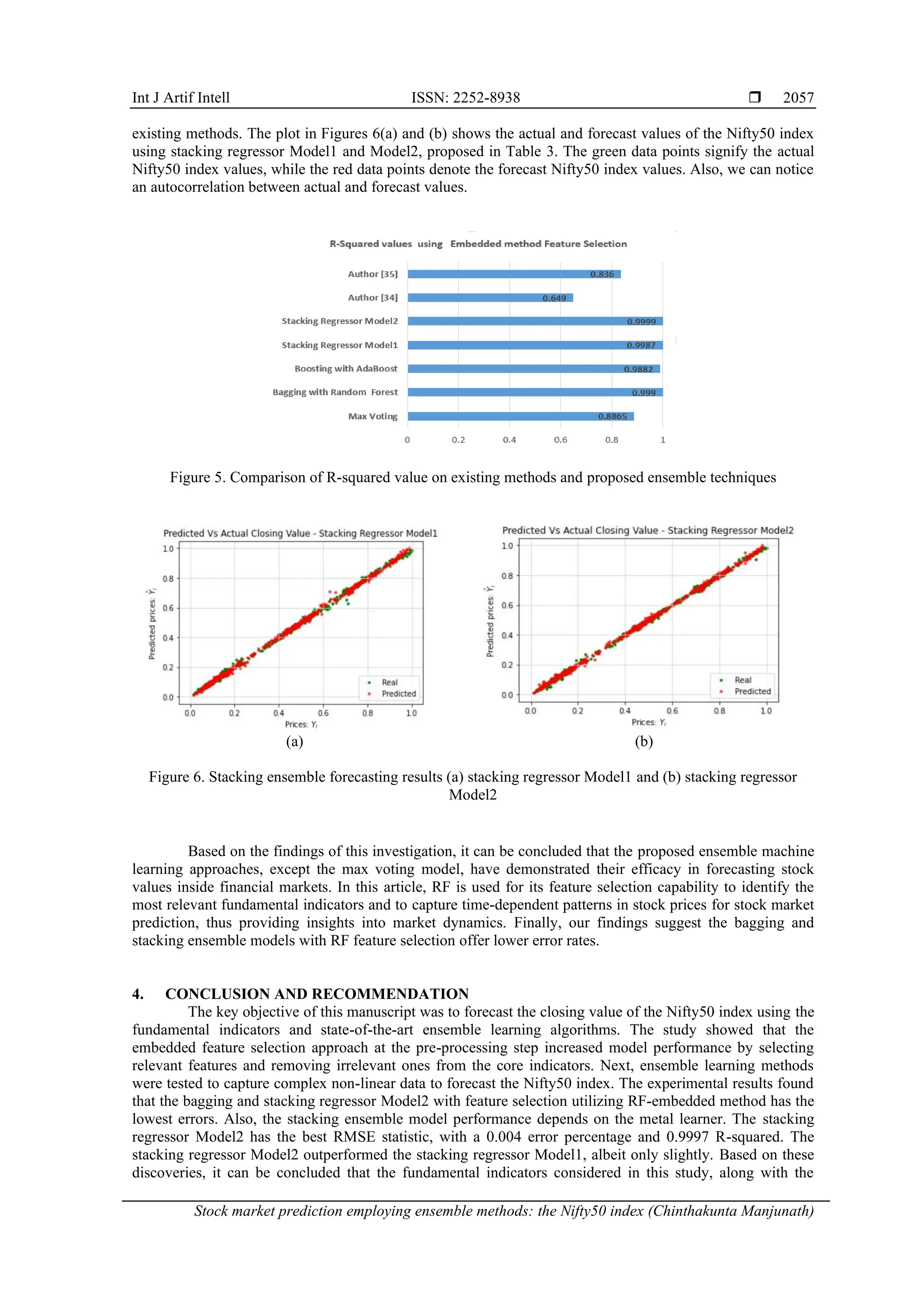
The R-squared value on existing methods and proposed ensemble techniques using the embedded
method-RF feature selection is shown in Figure 5. The bagging with RF model offers significantly higher
performance with R-squared value of 0.9990, which indicates it explains almost all of the variance in the
data. It performs exceptionally well in this scenario. The stacking regressor models (Model1 and Model2)
have higher R-squared values and are very close to 1 (0.9987 and 0.9999, respectively), indicating they
almost perfectly explain the variance in the data. These models continue to be the best performers. Figure 5
shows the proposed ensemble technique’s higher performance in terms of the R-squared metric compared to

2057
existing methods. The plot in Figures 6(a) and (b) shows the actual and forecast values of the Nifty50 index
using stacking regressor Model1 and Model2, proposed in Table 3. The green data points signify the actual
Nifty50 index values, while the red data points denote the forecast Nifty50 index values. Also, we can notice
an autocorrelation between actual and forecast values.
Figure 5. Comparison of R-squared value on existing methods and proposed ensemble techniques
(a) (b)
Figure 6. Stacking ensemble forecasting results (a) stacking regressor Model1 and (b) stacking regressor
Model2
Based on the findings of this investigation, it can be concluded that the proposed ensemble machine
learning approaches, except the max voting model, have demonstrated their efficacy in forecasting stock
values inside financial markets. In this article, RF is used for its feature selection capability to identify the
most relevant fundamental indicators and to capture time-dependent patterns in stock prices for stock market
prediction, thus providing insights into market dynamics. Finally, our findings suggest the bagging and
stacking ensemble models with RF feature selection offer lower error rates.
4. CONCLUSION AND RECOMMENDATION
The key objective of this manuscript was to forecast the closing value of the Nifty50 index using the
fundamental indicators and state-of-the-art ensemble learning algorithms. The study showed that the
embedded feature selection approach at the pre-processing step increased model performance by selecting
relevant features and removing irrelevant ones from the core indicators. Next, ensemble learning methods
were tested to capture complex non-linear data to forecast the Nifty50 index. The experimental results found
that the bagging and stacking regressor Model2 with feature selection utilizing RF-embedded method has the
lowest errors. Also, the stacking ensemble model performance depends on the metal learner. The stacking
regressor Model2 has the best RMSE statistic, with a 0.004 error percentage and 0.9997 R-squared. The
stacking regressor Model2 outperformed the stacking regressor Model1, albeit only slightly. Based on these
discoveries, it can be concluded that the fundamental indicators considered in this study, along with the

 ISSN: 2252-8938
2058
proposed feature selection techniques and ensemble learning models, offer an effective tool for forecasting
the Nifty50 index in the stock market. The study provides valuable insights for financial investors,
highlighting the advantages of employing ensemble machine-learning approaches for accurate and reliable
stock market predictions. The system can be further enhanced in future work by incorporating deep learning
and technical analysis techniques to create a more precise and reliable stock market forecasting system.
REFERENCES
[1] L. Bachelier, “Mathematical game theory (in French: Théorie mathématique du jeu),” Annales scientifiques de l’École normale
supérieure, vol. 18, pp. 143–209, 1901, doi: 10.24033/asens.493.
[2] M. Davis and A. Etheridge, Louis Bachelier’s ’theory of speculation, Princeton, USA: Princeton University Press, 2006.
[3] E. F. Fama, “Efficient capital markets: A review of theory and empirical work,” The Journal of Finance, vol. 25, no. 2, pp. 383-
417, 1970, doi: 10.2307/2325486.
[4] C. Manjunath, M. Balamurugan, B. Ghosh, and A. V. N. Krishna, “A review of stock market analysis approaches and forecasting
techniques,” in Smart Computing, 2021, pp. 368–382, doi: 10.1201/9781003167488-42.
[5] M. S. Checkley, D. A. Higón, and H. Alles, “The hasty wisdom of the mob: How market sentiment predicts stock market
behavior,” Expert Systems with Applications, vol. 77, pp. 256–263, Jul. 2017, doi: 10.1016/j.eswa.2017.01.029.
[6] M.-F. Tsai and C.-J. Wang, “On the risk prediction and analysis of soft information in finance reports,” European Journal of
Operational Research, vol. 257, no. 1, pp. 243–250, Feb. 2017, doi: 10.1016/j.ejor.2016.06.069.
[7] V. Drakopoulou, “A review of fundamental and technical stock analysis techniques,” Journal of Stock and Forex Trading, vol. 5,
no. 1, pp. 1-8, 2016, doi: 10.4172/2168-9458.1000163.
[8] E. E. Peters, Fractal market analysis: applying chaos theory to investment and economics. Third Avenue, New York: John Wiley
and Sons, 1994.
[9] A. W. Lo and A. C. MacKinlay, “Stock market prices do not follow random walks: evidence from a simple specification test,”
Review of Financial Studies, vol. 1, no. 1, pp. 41–66, Jan. 1988, doi: 10.1093/rfs/1.1.41.
[10] J. B. De Long, A. Shleifer, L. H. Summers, and R. J. Waldmann, “Noise trader risk in financial markets,” Journal of political
Economy, vol. 98, no. 4, pp. 703–738, 1990.
[11] J. R. Nofsinger, “Social mood and financial economics,” Journal of Behavioral Finance, vol. 6, no. 3, pp. 144–160, 2005, doi:
10.1207/s15427579jpfm0603_4.
[12] A. Shleifer and R. W. Vishny, “The limits of arbitrage,” The Journal of Finance, vol. 52, no. 1, pp. 35–55, Mar. 1997, doi:
10.1111/j.1540-6261.1997.tb03807.x.
[13] V. Tripathi and R. Seth, “Stock market performance and macroeconomic factors: the study of Indian equity market,” Global
Business Review, vol. 15, no. 2, pp. 291–316, 2014, doi: 10.1177/0972150914523599.
[14] S. Mbulawa, “Effect of macroeconomic variables on economic growth in botswana,” Journal of Economics and Sustainable
Development, vol. 6, no. 4, pp. 68-77, 2015.
[15] S. Mishra and S. Dhole, “Stock price comovement: evidence from India,” Emerging Markets Finance and Trade, vol. 51, no. 5,
pp. 893–903, Sep. 2015, doi: 10.1080/1540496X.2015.1061381.
[16] M. P. Yadav, A. Khera, and N. Mishra, “Empirical relationship between macroeconomic variables and stock market: evidence
from India,” Management and Labour Studies, vol. 47, no. 1, pp. 119–129, Feb. 2022, doi: 10.1177/0258042X211053166.
[17] G. Kutty, “The relationship between exchange rates and stock prices: the case of Mexico,” North American Journal of Finance
and Banking Research, vol. 4, no. 4, pp. 1–12, 2010.
[18] M. Srivastava and G. D. Sharma, “Risk and return linkages among stock markets of selected Asian countries,” TSME Jourrnal of
Management, vol. 6, pp. 1–16, 2016.
[19] B. Bodla and A. Amita, “Impact of macroeconomic factors on stock market return-a case study of India,” GGGI Management
Review, vol. 7, pp. 1–8, 2017.
[20] I. Berezinets, Y. Ilina, M. Smirnov, and L. Bulatova, “How does stock market react to dividend surprises? evidence from
emerging markets of India and Russia,” Journal of Asia-Pacific Business, vol. 18, no. 3, pp. 153–179, Jul. 2017, doi:
10.1080/10599231.2017.1346407.
[21] P. Misra, “An investigation of the macroeconomic factors affecting the Indian stock market,” Australasian Accounting, Business
and Finance Journal, vol. 12, no. 2, pp. 71–86, 2018, doi: 10.14453/aabfj.v12i2.5.
[22] S. Patel, “The effect of macroeconomic determinants on the performance of the Indian stock market,” NMIMS Management
Review, vol. 22, pp. 117-127, 2012.
[23] R. Gopinathan and S. R. S. Durai, “Stock market and macroeconomic variables: new evidence from India,” Financial Innovation,
vol. 5, no. 1, pp. 1-17, 2019, doi: 10.1186/s40854-019-0145-1.
[24] T. S. Quah, “DJIA stock selection assisted by neural network,” Expert Systems with Applications, vol. 35, no. 1–2, pp. 50–58,
2008, doi: 10.1016/j.eswa.2007.06.039.
[25] B. Graham and D. L. Dodd, Security Analysis: Principles and Technique, USA: McGraw Hill, vol. 36, no. 1. 1934.
[26] N. Milosevic, “Equity forecast: Predicting long term stock price movement using machine learning,” Journal of Economics
Library, pp. 288-294, 2016, doi: 10.1453/jel.v3i2.750.
[27] B. Ghosh, “Bankruptcy modelling of Indian public sector banks,” International Journal of Applied Behavioral Economics, vol. 6,
no. 2, pp. 52–65, Apr. 2017, doi: 10.4018/IJABE.2017040104.
[28] Y. Guo, F.-L. Chung, G. Li, and L. Zhang, “Multi-label bioinformatics data classification with ensemble embedded feature
selection,” IEEE Access, vol. 7, pp. 103863–103875, 2019, doi: 10.1109/ACCESS.2019.2931035.
[29] M. A. Siddiqi and W. Pak, “Optimizing filter-based feature selection method flow for intrusion detection system,” Electronics,
vol. 9, no. 12, pp. 1–18, 2020, doi: 10.3390/electronics9122114.
[30] V. Vapnik and C. Cortes, “Support-vector networks,” Machine Learning, vol. 20, pp. 273–297, 1995, doi: 10.1007/BF00994018.
[31] X. Tao et al., “Self-adaptive cost weights-based support vector machine cost-sensitive ensemble for imbalanced data
classification,” Information Sciences, vol. 487, pp. 31–56, Jun. 2019, doi: 10.1016/j.ins.2019.02.062.
[32] Y. Li and W. Chen, “A comparative performance assessment of ensemble learning for credit scoring,” Mathematics, vol. 8, no.
10, pp. 1-19, Oct. 2020, doi: 10.3390/math8101756.
[33] I. K. Nti, A. F. Adekoya, and B. A. Weyori, “A comprehensive evaluation of ensemble learning for stock-market prediction,”
Journal of Big Data, vol. 7, no. 1, pp. 1-40, Dec. 2020, doi: 10.1186/s40537-020-00299-5.

2059
[34] P. Aggarwal and N. Saqib, “Impact of macro economic variables of India and USA on Indian stock market,” International
Journal of Economics and Financial Issues, vol. 7, no. 4, pp. 10–14, 2017.
[35] H. Grigoryan, “A stock market prediction method based on support vector machines (SVM) and independent component analysis
(ICA),” Database Systems Journal, vol. 7, no. 1, pp. 12–21, 2016.
BIOGRAPHIES OF AUTHORS
Chinthakunta Manjunath received a Bachelor of Engineering from PESIT,
VTU, Bengaluru, in the field of Information Science and Engineering in 2007, and a Master of
Technology from RVCE, VTU, Bengaluru, in the field of Computer Science Engineering in
2011. He is currently an assistant professor in the Department of Computer Science and
Engineering, Christ (Deemed to be University), Bengaluru. His work focuses on the use of
machine learning and deep learning to predict stock market movements in the equity market.
He can be contacted at email: manju.chintell@gmail.com.
Balamurugan Marimuthu received his Ph.D. degree in Computer Science from
Anna University in Chennai, Tamil Nadu, India. He is an associate professor in the
Department of Computer Science and Engineering, Christ (Deemed to be a University),
Bengaluru. Financial market forecasts, wireless networks, deep learning, and machine learning
applications are all areas of study that interest him. He can be contacted at email:
balamurugan.m@christuniversity.in.
Bikramaditya Ghosh holds a Ph.D. in Financial Econometrics from Jain
University. He presently holds the position of professor at Symbiosis Institute of Business
Management (SIBM), Symbiosis International (Deemed University), in Bengaluru, India. He
was an ex. investment banker turned applied finance and analytics researcher and practitioner.
He has worked in private and foreign banks, including Citi and Standard Chartered for over
eleven years, gaining experience in both mid- and senior-level positions. He has published
more than twenty international research papers in finance and economics in journals of repute.
He is proficient in various analytical software. He has an Erasmus+grant to his credit. He has
attended international staff week at Vives University College, Kortrijk, Belgium. He can be
contacted at email: bikram77777@gmail.com.

Stock market prediction employing ensemble methods: the Nifty50 index

More Related Content

Similar to Stock market prediction employing ensemble methods: the Nifty50 index

More from IAESIJAI

Recently uploaded

Stock market prediction employing ensemble methods: the Nifty50 index