The document presents a statistical analysis involving multiple regression and two-way ANOVA focused on air quality data from Dublin City and the religious dedication across different age groups and genders. It discusses the data sources, objectives, statistical methods applied, results, and findings from the analyses, highlighting significant relationships and lack of significant effects in certain variables. Key findings include a strong correlation between PM10 and PM2.5, as well as the influence of age and gender on religious dedication.

1. STATISTICS REPORT
On
Multiple Regression and Two Way Annova
By:Siddharth Chaudhary
X16137001
Msc in Data Analytics
National College of Ireland

2. Table of Contents
MULTIPLE REGRESSION ANALYSIS........................................................................................................2
DATA SOURCE ..................................................................................................................................2
OBJECTIVE........................................................................................................................................2
DATA INFORMATION........................................................................................................................2
DATA CLEAN UP................................................................................................................................3
SOFTWARE.......................................................................................................................................3
ANALYSIS..........................................................................................................................................3
DATA SUMMARY .........................................................................................................................3
CORRELATION MATRIX................................................................................................................4
MULTIPLE REGRESSION ANALYSIS...............................................................................................5
RESIDUAL PLOT ...........................................................................................................................6
Model Summary .........................................................................................................................6
ANNOVA ...............................................................................................................................................7
OBJECTIVE........................................................................................................................................7
DATA INFORMATION........................................................................................................................7
SOFTWARE.......................................................................................................................................7
ANALYSIS.........................................................................................................................................8
DESCRIPTIVE STATISTICS .............................................................................................................8
LEVENE’S TEST ............................................................................................................................8
INTERATION EFFECT....................................................................................................................9
POST-HOC TEST.........................................................................................................................10
PLOT..........................................................................................................................................11
RESULT ......................................................................................................................................11
REFERENCES..............................................................................................................................12

3. MULTIPLE REGRESSION ANALYSIS
DATA SOURCE
This analysis has been done on air quality data of Dublin City. The data source is as follows.
https://data.gov.ie/dataset/air-quality-monitoring-data-dublin-city.
The data was present in four different excel.
1) Dublin city council PM10 and PM2.5 2011.csv.
2) Dublin city council NO and NO2 2011.csv
3) Dublin city council SO2 2011.csv
4) Dublin city council CO 2011.csv
OBJECTIVE
The reason of choosing this data is because the pollution is increasing in all metro cities of world. In
some cities like Beijing and Delhi the air quality is so bad that environment have become like gas
chambers.
The Objective of this analysis is to
1) Study the various components of air quality
2) Study the impact of other factors on PM2.5 and PM10
3) To understanding the relationship between all of them.
DATA INFORMATION
This dataset provides the information about various components responsible for air pollution.
● Nitrogen di oxide (NO2),
● Nitrogen Oxide (NO),
● Sulphur di Oxide (SO2),
● Carbon mono oxide (CO)
● PM 2.5
● PM 10
The major component of air are Nitrogen, Oxygen and Water Vapour covering 98% of air content.
Rest of the gases are present in small quantity which vary according to the quality of air. The major
one responsible for degrading the quality of air are Carbon mono oxide, Nitrogen di oxide, Ozone,
Sulphur di oxide and Particles. Particles are also known as particulate matter or PM. It consists of
smoke, dirt, soot, dust etc. These particles are classified according to their size. Example PM 10
means particles whose size is between 10 µm and 2.5 µm. PM 2.5 means particles smaller than 2.5
µm.
In this dataset we have collected the air pollutant information in the region of Dublin for the year
2011.

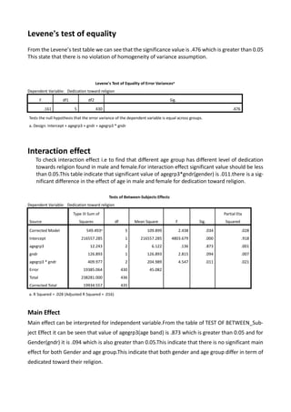
4. Data Type Granularity Converted
Nitrogen di oxide Hourly basis reading Daily average
Nitrogen Oxide Hourly basis reading Daily average
Sulphur di Oxide Hourly basis reading Daily average
Carbon mono oxide Hourly basis reading Daily average
PM2.5 Daily average none
PM 10 Daily average None
DATA CLEAN UP
The dataset was present in 5 different excel. So following clean up steps were taken.
1. Daily average were calculated by adding 24 reading of one day and dividing it by 24 for nitrogen
di oxide, Nitrogen oxide, Sulphur di oxide, Carbon mono oxide.
2. PM 2.5 and PM 10 were present in daily average format so no changes were done.
3. After consolidating this data one csv file was prepared.
SOFTWARE
R is used for this data analysis and it is very convenient tool for analysis and graph generation.
Data was loaded into R with the help of read
table command as follows.
air<-read.table("/home/hadoop/air_ireland.csv", sep=",",header=T)
ANALYSIS[1]
DATA SUMMARY
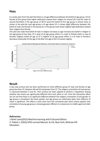
Below table represent the summary of the data in terms of max, min, median, 1st Quartile, 3 rd
Quartile. PM 2.5 and PM 10 are measured in g/m3. NO2, SO2, CO and NO are measured in ug/m3.

5. summary(air)
N02 NO SO2 CO PM2.5 PM10
Minimum 0.0 -2.2 0.0 0.0 0.1 2.2
1st Quartile 15.30 2.8 0.0 0.0 4.2 8.9
Median 28.50 10.8 0.2 0.1 6.3 11.4
Mean 32.97 25.86 0.4 0.07 8.6 14.39
3rd Quartile 48.0 27.3 0.5 0.1 9.6 15.80
Max 114.60 434.6 11.1 0.7 67.8 96.9
Count 365 365 365 365 365 365
CORRELATION MATRIX
library("PerformanceAnalytics")
my_data <- mtcars[, c(1,3,4,5,6,7)]
chart.Correlation(my_data, histogram=TRUE, pch=19)

6. The above fig displays the histogram of all variables, scatterplot of each pair and correlation
coefficient of each pair along with the p value significance.
AS we can see from the graph following pairs have strong relationship.
1. NO2 and NO
2. CO and NO
3. CO AND NO2
4 SO2 AND NO
3. PM 2.5 and PM 10
All these pairs are positively correlated to each other and coefficeint value is greater than .5. Rest of
the values are either very less or statistically not important as shows less significant p-value.
Multiple Regression Analysis
In this data we will perform multiple regression to identify the relationship between PM2.5/PM10
and NO, SO2 and CO.
Since NO2 and NO shows very strong relationship hence we choose only one of them. In this
experiment we analysed three models.
Regression 1 : lm(PM10~NO+SO2+CO-1, data=my_data)
Regression 2: lm(PM2.5~NO+SO2+CO-1, data=my_data)
Regression 3: lm(PM10~PM25+NO+SO2-1, data=my_data)
Model R2 P-value Residual error
PM25 ~ NO + SO2 + CO-1 27.96 *** 10.24
PM10 ~ NO + SO2 + CO-1 36.09 *** 14.35
PM10~PM25+CO+NO+SO2-1 85.12 *** 6.934

7. Statistical details of Regression 3 : PM10~PM2.5+CO+NO+SO2
Residuals:
Min 1Q Median 3Q Max
-49.923 -1.135 2.295 4.685 33.689
Coefficients:
Estimate Std. Error t value Pr(>|t|)
PM25 1.22785 0.03560 34.494 < 2e-16 ***
CO 18.93690 4.53754 4.173 3.76e-05 ***
NO -0.02241 0.01101 -2.035 0.0426 *
SO2 1.94215 0.47681 4.073 5.70e-05 ***
---
Signif. codes: 0 '***' 0.001 '**' 0.01 '*' 0.05 '.' 0.1 ' ' 1
Residual standard error: 6.934 on 361 degrees of freedom
Multiple R-squared: 0.8512, Adjusted R-squared: 0.8496
F-statistic: 516.4 on 4 and 361 DF, p-value: < 2.2e-16
As we can see from detailed statistics of regression the p-value of all coefficients except NO is very
significant. So CO , SO2 and PM2.5 impact is more significant in comparison to NO. The value of R
square is 85.12 which explains the 85 percent of variation in PM10 particle is explained by this
model.
RESIDUAL PLOT
In the residual plot we see it to be randomly scattered for values less than 20 but for greater than
20 we can see a positive pattern. So there are other factors which need to be captured to model
the variation.

8. Model Summary
We were trying to see the relationship between different variables as to establish the impact factor.
However in this data we did not find much relationship between PM2.5 and other chemical
properties and similarly PM10 and rest of chemical properties.
There is a strong relationship between PM10 and PM2.5. PM10 are the particles generated due to
smoke and dust. As the bigger particles rise, it becomes a reason of growth of PM2.5 which is quite
clear from the model. The smoke coming out of cars or factories consists of nitrogen and carbon
oxides and black carbon particles. They combine with air and make other compounds of Nitrogen
and oxygen. So as the smoke increases quantity of PM2.5 increases drastically.
Since Dublin is much less polluted in comparison to asian cities where PM2.5 has crossed the
bearable limit this effect is less visible.

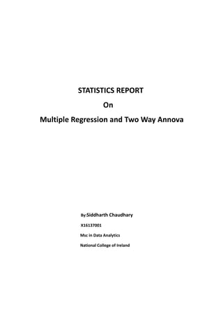
9. ANNOVA
In two-way analysis of variance, we need two categorical independent variables and one dependent
variable. Through two-way ANOVA we look at the individual and joint effect of two independent
variables on one dependent variable.
Data Source: Data Link: http://www.europeansocialsurvey.org/downloadwizard/?loggedin
OBJECTIVE
The data set is based on level of belief in their religion in different age bands of different gender in
Europe Union. The objectives of the test are:
• To find the different age band has different level of believe in their religion both in male and
female
• Gender differences of dedication toward their religions.
DATA VARIABLES
The independent variables gender is recoded as males = 1 and females = 2.
The age bands are recoded as:
Band 1: <= 37 yrs;
Band 2: 38-56 yrs;
Band3: >=58 yrs.
The dependent variable is Dedication toward religion which ranges: 5-35.
MEASUREMENTS
For measurement, there are two categorical independent variables (Gender and age band). The age
band has three bands. The level of Dedication toward religion is assigned in range from 5– 35. Dif-
ferent tests like Levene's test of equality, homogeneity tests and post hoc tests are performed.
SOFTWARE
For this analysis SPSS has been used.[2]

10. Output from two-way ANOVA
Descriptive statistics
It explains the mean, standard deviation and records for each group.It shows number of male and
female in all age group. There is not much difference between the std.deviation of the age
group,they are almost similar.The mean of age group for (<=37) is 22.28,mean of age group (38-56)
is 22.24 and mean of age group (57+) is 22.62.
Descriptive Statistics
Dependent Variable: Dedication toward religion
Age Group 3(Binned) Gender Mean Std. Deviation N
<= 37 Male 20.40 6.904 73
Female 24.23 6.483 71
Total 22.28 6.947 144
38 - 56 Male 22.27 6.852 62
Female 22.21 6.566 86
Total 22.24 6.664 148
57+ Male 22.88 6.959 69
Female 22.37 6.565 75
Total 22.62 6.738 144
Total Male 21.81 6.958 204
Female 22.88 6.574 232
Total 22.38 6.770 436

11. Levene's test of equality
From the Levene’s test table we can see that the significance value is .476 which is greater than 0.05
This state that there is no violation of homogeneity of variance assumption.
Levene's Test of Equality of Error Variancesa
Dependent Variable: Dedication toward religion
F df1 df2 Sig.
.161 5 430 .476
Tests the null hypothesis that the error variance of the dependent variable is equal across groups.
a. Design: Intercept + agegrp3 + gndr + agegrp3 * gndr
Interaction effect
To check interaction effect i.e to find that different age group has different level of dedication
towards religion found in male and female.For interaction effect significant value should be less
than 0.05.This table indicate that significant value of agegrp3*gndr(gender) is .011.there is a sig-
nificant difference in the effect of age in male and female for dedication toward religion.
Tests of Between-Subjects Effects
Dependent Variable: Dedication toward religion
Source
Type III Sum of
Squares df Mean Square F Sig.
Partial Eta
Squared
Corrected Model 549.493a 5 109.899 2.438 .034 .028
Intercept 216557.285 1 216557.285 4803.679 .000 .918
agegrp3 12.243 2 6.122 .136 .873 .001
gndr 126.893 1 126.893 2.815 .094 .007
agegrp3 * gndr 409.977 2 204.989 4.547 .011 .021
Error 19385.064 430 45.082
Total 238281.000 436
Corrected Total 19934.557 435
a. R Squared = .028 (Adjusted R Squared = .016)
Main Effect
Main effect can be interpreted for independent variable.From the table of TEST OF BETWEEN_Sub-
ject Effect it can be seen that value of agegrp3(age band) is .873 which is greater than 0.05 and for
Gender(gndr) it is .094 which is also greater than 0.05.This indicate that there is no significant main
effect for both Gender and age group.This indicate that both gender and age group differ in term of
dedicated toward their religion.

12. Effect size
The effect size for age group and Gender in partial eta column is less than 0.05.This effect size is
significantly different.
Post-hoc test
As per post hoc test there is no significant effect in religious
belief of male and female.
In TUKEY(honestly significant difference) test it shows there is no significant difference in the age
group as all the significant value is greater than 0.05.
Multiple Comparisons
Dependent Variable: Dedication toward religion
Tukey HSD
(I) Age Group 3(Binned) (J) Age Group 3(Binned)
Mean Differ-
ence (I-J) Std. Error Sig.
95% Confidence Interval
Lower Bound Upper Bound
<= 37 38 - 56 .05 .786 .998 -1.80 1.90
57+ -.33 .791 .907 -2.19 1.53
38 - 56 <= 37 -.05 .786 .998 -1.90 1.80
57+ -.38 .786 .878 -2.23 1.47
57+ <= 37 .33 .791 .907 -1.53 2.19
38 - 56 .38 .786 .878 -1.47 2.23
Based on observed means.
The error term is Mean Square(Error) = 45.082.

13. Plots
It is quite clear from the plot that there is a huge difference between the belief of age group <37.As
female of this group have higher dedication toward their religion its around 24.5 and for male its
around 20.4.Next is the age group of 38-57 years.The belief of this age group is almost same as
shown in the plot.the next age group is of age above 57+ it shows slight difference between the
belief of male and female in this group.As in this group male shows slightly high dedication toward
their religion than female.
This plot also state that belief of male in religion increases as age increases.but belief in religion in
the age group of less than 37 is least of all age group either it is male or female while in case of
females religious belief till age of 37 is highest of all age group either it is of male or female.it
decreases drastically till the age of 56.After the age of 56 it increases slightly.
Result
A two way annova test has been performed on three different group of male and female of age
group less than 37, between 38 and 56 and greater than 57. The religious orientation of each person
is measured between 5 and 35. Then annova has been applied to perform a hypothesis testing
whether two means are significantly different from each other or not. From the interaction effect
we can see that there is no significant different between the religious orientation if only gender or
age group is considered. But when gender and age group are collectively taken then different of
mean is significant. This effect is more clear from the cumulative plot which clearly explains that
orientation of young age group is showing greater different in comparison to middle aged and older
group.
References:
1.Brett Lantz(2013) Machine learning with R.Second Edition.
2. Pallant J. (2016) SPSS survival Manual. 6th Ed. New York, McGraw Hill
Education.