Mapping time-varying air quality using IDW and make an animation

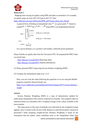
1. Muhammad Irsyadi Firdaus
P66067055
SPATIAL ENVIRONMETAL DATA ANALYSIS AND MODEL 1
Homework 2
Mapping time-varying air quality using IDW and make an animation. For example,
air quality maps are from 2017/2/6 9am to 2017/2/7 9am.
https://data.lass-net.org/LASS/assets/IDW_gif/Taiwan_latest_last_24h.gif
A general form of finding an interpolated value at a given point based on
samples for i= using IDW is an interpolating function:
d is a given distance; p is a positive real number, called the power parameter
Please find the air quality data from the Taiwanese EPA. We prepared the PM2.5 data
on current time.
http://data.gov.tw/node/6074 (Real-time data)
http://data.gov.tw/node/6075 (Station information)
(1) Please generate PM2.5 map using inverse distance weighting (IDW).
(2) Compare the interpolation maps at p=1 to 5.
Here, you can write the codes following the equations or we are using the Matlab
program created by Simone Fatichi, see
https://www.mathworks.com/matlabcentral/fileexchange/24477-inverse-distance-
weight
Answer
Inverse Distance Weighting (IDW) is a type of deterministic method for
multivariate interpolation with a known scattered set of points. The assigned values to
unknown points are calculated with a weighted average of the values available at the
known points.
The name given to this type of methods was motivated by the weighted average
applied, since it resorts to the inverse of the distance to each known point ("amount of
proximity") when assigning weights.Inverse Distance Weighting is based on the
assumption that the nearby values contribute more to the interpolated values than

2. Muhammad Irsyadi Firdaus
P66067055
SPATIAL ENVIRONMETAL DATA ANALYSIS AND MODEL 2
distant observations. In other words, for this method the influence of a known data point
is inversely related to the distance from the unknown location that is being estimated.
The advantage of IDW is that it is intuitive and efficient. This interpolation works best
with evenly distributed points. In order to improve the computational time is possible
to set bounds to the dispersion points that contribute to the calculation of the
interpolated value, to all those dispersion points within a given search radius centered
on the interpolated point.
Data obtained include station name, latitude coordinates, longitude coordinates,
PM 2.5 values and others. In this case, the air quality map uses the particulate matter
PM2.5 with different power values P=1, P=2, P=3, P=4, and P=5.
Figure 1. Air Quality Data From The Taiwanese EPA
Particulate matter (PM2.5) particles are air pollutants with a diameter less than 2.5
micrometers, small enough to invade even the smallest of airways in human body. Par-
ticulate matter pollutant is composed of a mixture of mi- croscopic solids and liquid
droplets suspended in air. Unlike most air pollutants that consist of only one chemical
compound, PM2.5 particles consist of multiple compounds and are formed from
primary and secondary participles.
Based on the results of interpolation of this data processing obtained a sufficient
understanding to support the existing literature review the greater the value of power
used, the results obtained increasingly centralized and have a low flattening.

3. Muhammad Irsyadi Firdaus
P66067055
SPATIAL ENVIRONMETAL DATA ANALYSIS AND MODEL 3
Table 1. Particulate matter statistics of the IDW method
Power
Parameter
Min Max Mean Std.Dev
1 2.33 25.00 7.33 1.39
2 0.03 25.00 6.92 2.12
3 0.00 25.00 6.55 2.70
4 0.00 25.00 6.30 3.07
5 0.00 25.00 6.14 3.32
Values of particulate matter statistics that include maximal values, minimum
values, the average value and the standard deviation value. In table 1 shows that the
greater the value of power parameters then the smaller the average value of Particulate
matter and the greater the value of power parameters then the standard deviation value
is greater.
The power value at this IDW interpolation determines the effect on the station
points, where the effect will be greater at the closer points resulting in a more detailed
surface. If the power value is reduced, the resulting surface is smoother. The weight
used for the average is the derivative of the distance function between the sample point
and the interpolated points.
Reference
Azpurua, M., and K. D. Ramos, 2010, “A Comparizon of Spatial Interpolation Methods
For Estimation of Average Electromagnetic Field Magnitude”. Progress in
Electromagnetics Research M., Vol. 14, pp. 135-145.
Chaplot, V., Darboux F., Bourennane H., 2006, “Accuracy of Interpolation Techniques
for The Derivation of Digital Elevation Models in Relation to Landform Type
and Data Density”, Geomorphology, Vol 77, pp. 126-141.
Childs C., 2004, Interpolating Surface in ArcGIS Spatial Analyst, ESRI Education
Services.

4. Muhammad Irsyadi Firdaus
P66067055
SPATIAL ENVIRONMETAL DATA ANALYSIS AND MODEL 4
Figure 2. PM 2.5 With Power 1

5. Muhammad Irsyadi Firdaus
P66067055
SPATIAL ENVIRONMETAL DATA ANALYSIS AND MODEL 5
Figure 3. PM 2.5 With Power 2

6. Muhammad Irsyadi Firdaus
P66067055
SPATIAL ENVIRONMETAL DATA ANALYSIS AND MODEL 6
Figure 4. PM 2.4 With Power 3

7. Muhammad Irsyadi Firdaus
P66067055
SPATIAL ENVIRONMETAL DATA ANALYSIS AND MODEL 7
Figure 5. PM 2.5 With Power 4

8. Muhammad Irsyadi Firdaus
P66067055
SPATIAL ENVIRONMETAL DATA ANALYSIS AND MODEL 8
Figure 6. PM 2.5 With Power 5