Sqlite

What Is SQLite?
SQLite is a public-domain software package that provides a relational database management
system, or RDBMS.
Relational database systems are used to store user-defined records in large tables. In addition to
data storage and management,a database engine can process complex query commands that
combine data from multiple tables to generate reports and data summaries

SQLite is lightweight when it comes to setup complexity, administrative overhead, and resource
usage
SQLite is remarkably flexible in both where it can be run and how it can be used. This
chapter will take a brief look at some of the roles SQLite is designed to fill. Some of
these roles are similar to those taken by traditional client/server RDBMS products.
Other roles take advantage of SQLite’s size and ease of use, offering solutions you might
not consider with a full client/server database.

SQLite is capable of creating databases that are held entirely in memory. This is extremely
useful for creating small, temporary databases that require no permanent
storage.
In-memory databases are often used to cache results pulled from a more traditional
RDBMS server. An application may pull a subset of data from the remote database,
place it into a temporary database, and then process multiple detailed searches and
refinements against the local copy. This is particularly useful when processing typeahead
suggestions, or any other interactive element that requires very quick response
times.

Archives and Data Stores
SQLite makes it very easy to package complex data sets into a single, easy-to-access,
fully cross-platform file. Having all the data in a single file makes it much easier to
distribute or download large, multi-table data stores, such as large dictionaries or geolocation
references.
Unlike many RDBMS products, the SQLite library is able to access read-only database
files. This allows data stores to be read directly from an optical disc or other read-only
filesystem. This is especially useful for systems with limited hard drive space, such as
video game consoles.

Client/Server Stand-in
SQLite works well as a “stand-in” database for those situations when a more robust
RDBMS would normally be the right choice, were it available. SQLite can be especially
useful for the demonstration and evaluation of applications and tools that normally
depend on a database.

Generic SQL Engine
SQLite virtual tables allow a developer to define the contents of a table through code.
By defining a set of callback functions that fetch and return rows and columns, a developer
can create a link between the SQLite data processing engine and any data
source. This allows SQLite to run queries against the data source without importing
the data into a standard table.

The SQLite code base supports all of these operating systems natively, and precompiled libraries and
executables for all three environments are available from the SQLite website
SQLite Products
The SQLite project consists of four major products:
SQLite core
The SQLite core contains the actual database engine and public API. The core can be built into a static
or dynamic library, or it can be built in directly to an application.
sqlite3 command-line tool
The sqlite3 application is a command-line tool that is built on top of the SQLite core. It allows a
developer to issue interactive SQL commands to the SQLite core. It is extremely useful for developing
and debugging queries.

Tcl extension
SQLite has a strong history with the Tcl language. This library is essentially a copy
of the SQLite core with the Tcl bindings tacked on. When compiled into a library,
this code exposes the SQLite interfaces to the Tcl language through the Tcl Extension
Architecture (TEA). Outside of the native C API, these Tcl bindings are the
only official programming interface supported directly by the SQLite team.

Building
There are a number of different ways to build SQLite, depending on what you’re trying
to build and where you would like it installed. If you are trying to integrate the SQLite
core into a host application, the easiest way to do that is to simply copy sqlite3.c and
sqlite3.h into your application’s source directory. If you’re using an IDE, the sqlite3.c
file can simply be added to your application’s project file and configured with the proper
search paths and build directives. If you want to build a custom version of the SQLite
library or sqlite3 utility, it is also easy to do that by hand.

Configure
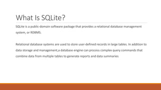
If you’re using the Unix amalgamation distribution, you can build and install SQLite
using the standard configure script. After downloading the distribution, it is fairly easy
to unpack, configure, and build the source:
$ tar xzf sqlite-amalgamation-3.x.x.tar.gz
$ cd sqlite-3.x.x
$ ./configure
[...]
$ make

An sqlite3 Primer
Once you have some form of SQLite installed, the first step is normally to run
sqlite3 and play around. The sqlite3 tool accepts SQL commands from an interactive
prompt and passes those commands to the SQLite core for processing.
Even if you have no intention of distributing a copy of sqlite3 with your application,
it is extremely useful to have a copy around for testing and debugging queries. If your
application uses a customized build of the SQLite core, you will likely want to build a
copy of sqlite3 using the same build parameters.
To get started, just run the SQLite command. If you provide a filename (such as
test.db), sqlite3 will open (or create) that file. If no filename is given, sqlite3 will
automatically open an unnamed temporary database

$ sqlite3 test.db
SQLite version 3.6.23.1
Enter ".help" for instructions
Enter SQL statements terminated with a ";"
sqlite>

The SQL Language
Structured Query Language, or SQL. Although sometimes pronounced “sequel,” the official
pronunciation is to name each letter as “ess-cue-ell.” The SQL language is the main means of
interacting with nearly all modern relational database systems. SQL provides commands to
configure the tables, indexes, and other data structures within the database. SQL commands are
also used to insert, update, and delete data records, as well as query those records to look up
specific data values.

All interaction with a relational database is done through the SQL language. This is
true when interactively typing commands or when using the programming API. In all
cases, data is stored, modified, and retrieved through SQL commands.

Learning SQL
For people just getting started, the most important commands are CREATE TABLE,
INSERT, and SELECT. These will let you create a table, insert some data into the table,
and then query the data and display it.

Brief Background
Although the first official SQL specification was published in 1986 by the American
National Standards Institute (ANSI), the language traces its roots back to the early
1970s and the pioneering relational database work that was being done at IBM. Current
SQL standards are ratified and published by the International Standards Organization
(ISO).

Declarative
The core of SQL is a declarative language. In a declarative language, you state what you
want the results to be and allow the language processor to figure out how to deliver the
desired results. Compare this to imperative languages, such as C, Java, Perl, or Python,
where each step of a calculation or operation must be explicitly written out, leaving it
up to the programmer to lead the program, step by step, to the correct conclusion.

Portability
SQL’s biggest flaw is that formal standardization has almost always followed common
implementations. Almost every database product (including SQLite) has custom extensions
and enhancements to the core language that help differentiate it from other
products, or expose features or control systems that are not covered by the core SQL
standard. Often these enhancements are related to performance enhancements, and
can be difficult to ignore.

Basic Syntax
SQL consists of a number of different commands, such as CREATE TABLE or INSERT. These
commands are issued and processed one at a time.
Although it is customary to use all capital letters for SQL commands and keywords,
SQL is a case-insensitive* language.

Three-Valued Logic
SQL allows any value to be assigned a NULL. NULL is not a value in itself (SQLite
actually implements it as a unique valueless type), but is used as a marker or flag to
represent unknown or missing data. The thought is that there are times when values
for a specific row element may not be available or may not be applicable.

A NULL may not be a value, but it can be assigned to data elements that normally have
values, and can therefore show up in expressions. The problem is that NULLs don’t
interact well with other values. If a NULL represents an unknown that might be any
possible value, how can we know if the expression NULL > 3 is true or false?

SQL Data Languages
SQL commands are divided into four major categories, or languages. Each language
defines a subset of commands that serve a related purpose. The first language is the
Data Definition Language, or DDL, which refers to commands that define the structure
of tables, views, indexes, and other data containers and objects within the database.
CREATE TABLE (used to define a new table) and DROP VIEW (used to delete a view) are
examples of DDL commands.

The second category of commands is known as Data Manipulation Language, or
DML. These are all of the commands that insert, update, delete, and query actual data
values from the data structures defined by the DDL. INSERT (used to insert new values
into a table) and SELECT (used to query or look up data from tables) are examples of
DML commands.

Data Definition Language
The DDL is used to define the structure of data containers and objects within the database.
The most common of these containers and objects are tables, indexes, and
views. As you’ll see, most objects are defined with a variation of the CREATE command,
such as CREATE TABLE or CREATE VIEW. The DROP command is used to delete an existing
object (and all of the data it might contain). Examples include DROP TABLE or DROP
INDEX. Because the command syntax is so different, statements like CREATE TABLE or
CREATE INDEX are usually considered to be separate commands, and not variations of a
single CREATE command

The basics
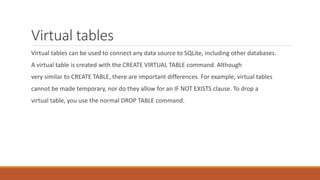
The most basic syntax for CREATE TABLE looks something like this:
CREATE TABLE table_name
(
column_name column_type,
[...]
);
A table name must be provided to identify the new table. After that, there is just a simple
list of column names and their types. Table names come from a global namespace of
all identifiers, including the names of tables, views, and indexes.

Column types
Most databases use strong, static column typing. This means that the elements of a
column can only hold values compatible with the column’s defined type. SQLite utilizes
a dynamic typing technique known as manifest typing. For each row value, manifest
typing records the value’s type along with the value data. This allows nearly any element
of any row to hold almost any type of value.

In the strictest sense, SQLite supports only five concrete datatypes. These are known
as storage classes, and represent the different ways SQLite might choose to store data
on disk. Every value has one of these five native storage classes:
NULL
A NULL is considered its own distinct type. A NULL type does not hold a value.
Literal NULLs are represented by the keyword NULL

Integer
A signed integer number. Integer values are variable length, being 1, 2, 3, 4, 6, or
8 bytes in length, depending on the minimum size required to hold the specific
value. Integer have a range of −9,223,372,036,854,775,808 to +9,223,372,
036,854,775,807, or roughly 19 digits. Literal integers are represented by any bare
series of numeric digits (without commas) that does not include a decimal point
or exponent.

Float
A floating-point number, stored as an 8-byte value in the processor’s native format.
For nearly all modern processors, this is an IEEE 754 double-precision number.
Literal floating-point numbers are represented by any bare series of numeric digits
that include a decimal point or exponent.

Text
A variable-length string, stored using the database encoding (UTF-8, UTF-16BE,
or UTF-16LE). Literal text values are represented using character strings in single
quotes.
BLOB
A length of raw bytes, copied exactly as provided. Literal BLOBs are represented
as hexadecimal text strings preceded by an x. For example, the notation
x'1234ABCD' represents a 4-byte BLOB. BLOB stands for Binary Large OBject.

Each table column must have one of five type affinities:
Text
A column with a text affinity will only store values of type NULL, text, or BLOB.
If you attempt to store a value with a numeric type (float or integer) it will be
converted into a text representation before being stored as a text value type.

Numeric
A column with a numeric affinity will store any of the five types. Values with integer
and float types, along with NULL and BLOB types, are stored without conversion.
Any time a value with a text type is stored, an attempt is made to convert the value
to a numeric type (integer or float). Assuming the conversion works, the value is
stored in an appropriate numeric type. If the conversion fails, the text value is stored
without any type of conversion.

Integer
A column with an integer affinity works essentially the same as a numeric affinity.
The only difference is that any value with a float type that lacks a fractional component
will be converted into an integer type
Float
A column with a floating-point affinity also works essentially the same as a numeric
affinity. The only difference is that most values with integer types are converted
into floating-point values and stored as a float type.

None
A column with a none affinity has no preference over storage class. Each value is
stored as the type provided, with no attempt to convert anything.

Column constraints
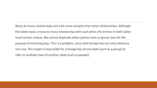
In addition to column names and types, a table definition can also impose constraints
on specific columns or sets of columns. A more complete view of the CREATE TABLE
command looks something like this:
CREATE TABLE table_name
(
column_name column_type column_constraints...,
[... ,]
table_constraints,
[...]
);

Primary keys
In addition to these other constraints, a single column (or set of columns) can be designated
as the PRIMARY KEY. Each table can have only one primary key. Primary keys
must be unique, so designating a column as PRIMARY KEY implies the UNIQUE constraint
as well, and will result in an automatic unique index being created. If a column is
marked both UNIQUE and PRIMARY KEY, only one index will be created

In SQLite, PRIMARY KEY does not imply NOT NULL. This is in contradiction to the SQL
standard and is considered a bug, but the behavior is so long-standing that there are
concerns about fixing it and breaking existing applications. As a result, it is always a
good idea to explicitly mark at least one column from each PRIMARY KEY as NOT NULL.

Table constraints
Table definitions can also include table-level constraints. In general, table constraints
and column constraints work the same way. Table-level constraints still operate on
individual rows. The main difference is that using the table constraint syntax, you can
apply the constraint to a group of columns rather than just a single column. It is perfectly
legal to define a table constraint with only one column, effectively defining a column
constraint. Multicolumn constraints are sometimes known as compound constraints

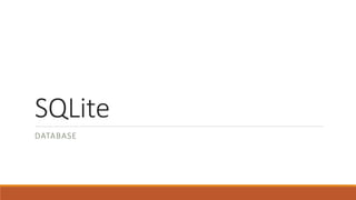
Consider a table that contains records of all the rooms in a multibuilding campus:
CREATE TABLE rooms
(
room_number INTEGER NOT NULL,
building_number INTEGER NOT NULL,
[...,]
PRIMARY KEY( room_number, building_number )
);

Tables from queries
You can also create a table from the output of a query. This is a slightly different CREATE
TABLE syntax that creates a new table and preloads it with data, all in one command:
CREATE [TEMP] TABLE table_name AS SELECT query_statement;
Using this form, you do not designate the number of columns or their names or types.
Rather, the query statement is run and the output is used to define the column names
and preload the new table with data.

Altering tables
SQLite supports a limited version of the ALTER TABLE command. Currently, there are
only two operations supported by ALTER TABLE: add column and rename. The add column
variant allows you to add new columns to an existing table. It cannot remove
them. New columns are always added to the end of the column list. Several other
restrictions apply.

Dropping tables
The CREATE TABLE command is used to create tables and DROP TABLE is used to delete
them. The DROP TABLE command deletes a table and all of the data it contains. The table
definition is also removed from the database system catalogs.
The DROP TABLE command is very simple. The only argument is the name of the table
you wish to drop:
DROP TABLE table_name;

Virtual tables
Virtual tables can be used to connect any data source to SQLite, including other databases.
A virtual table is created with the CREATE VIRTUAL TABLE command. Although
very similar to CREATE TABLE, there are important differences. For example, virtual tables
cannot be made temporary, nor do they allow for an IF NOT EXISTS clause. To drop a
virtual table, you use the normal DROP TABLE command.

Views
Views provide a way to package queries into a predefined object. Once created, views
act more or less like read-only tables. Just like tables, new views can be marked as
TEMP, with the same result. The basic syntax of the CREATE VIEW command is:
CREATE [TEMP] VIEW view_name AS SELECT query_statement

Row Modification Commands
INSERT
The INSERT command is used to create new rows in the specified table. There are two
meaningful versions of the command. The first version uses a VALUES clause to specify
a list of values to insert:
INSERT INTO table_name (column_name [, ...]) VALUES (new_value [, ...]);

UPDATE
The UPDATE command is used to assign new values to one or more columns of existing
rows in a table. The command can update more than one row, but all of the rows must
be part of the same table. The basic syntax is:
UPDATE table_name SET column_name=new_value [, ...] WHERE expression

DELETE
As you might guess, the DELETE command is used to delete or remove one or more rows
from a single table. The rows are completely deleted from the table:
DELETE FROM table_name WHERE expression;

The Query Command
The final DML command to cover is the SELECT command. SELECT is used to extract or
return values from the database. Almost any time you want to extract or return some
kind of value, you’ll need to use the SELECT command. Generally, the returned values
are derived from the contents of the database, but SELECT can also be used to return the
value of simple expressions. This is a great way to test out expressions, for example:
sqlite> SELECT 1+1, 5*32, 'abc'||'def', 1>2;
1+1 5*32 'abc' || 'def' 1>2
---------- ---------- -------------- ----------
2 160 abcdef 0

Consider this table:
sqlite> CREATE TABLE tbl ( a, b, c, id INTEGER PRIMARY KEY );
sqlite> INSERT INTO tbl ( a, b, c ) VALUES ( 10, 10, 10 );

sqlite> SELECT * FROM tbl;
a b c id
---------- ---------- ---------- ----------
10 10 10 1
11 15 20 2
12 20 30 3

sqlite> SELECT a, c FROM tbl;
a c
---------- ----------
10 10
11 20
12 30

The SELECT Command
The SELECT command is used to extract data from the database. Any time you want to
query or return user data stored in a database table, you’ll need to use the SELECT
Command

SQL Tables
The main SQL data structure is the table. Tables are used for both storage and for data
manipulation. We’ve seen how to define tables with the CREATE TABLE command, but
let’s look at some of the details.
A table consists of a heading and a body. The heading defines the name and type (in
SQLite, the affinity) of each column. Column names must be unique within the table.
The heading also defines the order of the columns, which is fixed as part of the table
definition

The SELECT Pipeline
The SELECT syntax tries to represent a generic framework that is capable of expressing
many different types of queries. To achieve this, SELECT has a large number of optional
clauses, each with its own set of options and formats.
The most general format of a standalone SQLite SELECT statement looks like this:
SELECT [DISTINCT] select_heading
FROM source_tables
WHERE filter_expression
GROUP BY grouping_expressions
HAVING filter_expression
ORDER BY ordering_expressions
LIMIT count
OFFSET count

CROSS JOIN
A CROSS JOIN matches every row of the first table with every row of the second table. If
the input tables have x and y columns, respectively, the resulting table will have x+y
columns. If the input tables have n and m rows, respectively, the resulting table will
have n·m rows. In mathematics, a CROSS JOIN is known as a Cartesian product.
The syntax for a CROSS JOIN is quite simple:
SELECT ... FROM t1 CROSS JOIN t2 ...

shows how a CROSS JOIN is calculated.
Because CROSS JOINs have the potential to generate extremely large tables, care must
be taken to only use them when appropriate.

If the input tables have C and D columns, respectively, a JOIN...ON will always result
in C+D columns.
The conditional expression can be used to test for anything, but the most common type
of expression tests for equality between similar columns in both tables. For example,
in a business employee database, there is likely to be an employee table that contains
(among other things) a name column and an eid column (employee ID number). Any
other table that needs to associate rows to a specific employee will also have an eid
column that acts as a pointer or reference to the correct employee. This relationship
makes it very common to have queries with ON expressions similar to:
SELECT ... FROM employee JOIN resource ON employee.eid = resource.eid ...

This query will result in an output table where the rows from the resource table are
correctly matched to their corresponding rows in the employee table.
This JOIN has two issues. First, that ON condition is a lot to type out for something so
common. Second, the resulting table will have two eid columns, but for any given row,
the values of those two columns will always be identical. To avoid redundancy and
keep the phrasing shorter, inner join conditions can be declared with a USING expression.
This expression specifies a list of one or more columns:
SELECT ... FROM t1 JOIN t2 USING ( col1 ,... ) ...
Queries from the employee database would now look something like this:
SELECT ... FROM employee JOIN resource USING ( eid ) ...

OUTER JOIN
The OUTER JOIN is an extension of the INNER JOIN. The SQL standard defines three types
of OUTER JOINs: LEFT, RIGHT, and FULL. Currently, SQLite only supports the LEFT OUTER
JOIN.
OUTER JOINs have a conditional that is identical to INNER JOINs, expressed using an ON,
USING, or NATURAL keyword. The initial results table is calculated the same way. Once
the primary JOIN is calculated, an OUTER join will take any unjoined rows from one or

both tables, pad them out with NULLs, and append them to the resulting table. In the
case of a LEFT OUTER JOIN, this is done with any unmatched rows from the first table
(the table that appears to the left of the word JOIN)

Table aliases
Because the JOIN operator combines the columns of different tables into one, larger
table, there may be cases when the resulting working table has multiple columns with
the same name. To avoid ambiguity, any part of the SELECT statement can qualify any
column reference with a source-table name. However, there are some cases when this
is still not enough. For example, there are some situations when you need to join a table
to itself, resulting in the working table having two instances of the same source-table.
Not only does this make every column name ambiguous, it makes it impossible to
distinguish them using the source-table name. Another problem is with subqueries, as
they don’t have concrete source-table names.

To avoid ambiguity within the SELECT statement, any instance of a source-table, view, or subquery
can be assigned an alias. This is done
with the AS keyword. For example, in the cause of a self-join, we can assign a unique alias for each
instance of the same table:
SELECT ... FROM x AS x1 JOIN x AS x2 ON x1.col1 = x2.col2 ...
Or, in the case of a subquery:
SELECT ... FROM ( SELECT ... ) AS sub ...
Technically, the AS keyword is optional, and each source-table name can simply be followed with an
alias name. This can be quite confusing, however, so it is recommended you use the AS keyword.
If any of the subquery columns conflict with a column from a standard source table, you can now use
the sub qualifier as a table name. For example, sub.col1. Once a table alias has been assigned, the
original source-table name becomes invalid and cannot be used as a column qualifier. You must use
the alias instead.

WHERE Clause
The WHERE clause is used to filter rows from the working table generated by the FROM
clause. It is very similar to the WHERE clause found in the UPDATE and DELETE commands.
An expression is provided that is evaluated for each row. Any row that causes the
expression to evaluate to false or NULL is discarded. The resulting table will have the
same number of columns as the original table

Some WHERE clauses can get quite complex, resulting in a long series of AND operators
used to join sub-expressions together. Most filter for a specific row, however, searching
for a specific key value.

GROUP BY Clause
The GROUP BY clause is used to collapse, or “flatten,” groups of rows. Groups can be
counted, averaged, or otherwise aggregated together. If you need to perform any kind
of inter-row operation that requires data from more than one row, chances are you’ll
need a GROUP BY.
The GROUP BY clause provides a list of grouping expressions and optional collations.
Very often the expressions are simple column references, but they can be arbitrary
expressions. The syntax looks like this:
GROUP BY grouping_expression [COLLATE collation_name] [,...]

SELECT Header
The SELECT header is used to define the format and content of the final result table. Any column
you want to appear in the final results table must be defined by an expression in the SELECT
header. The SELECT heading is the only required step in the SELECT command
pipeline.The format of the header is fairly simple, consisting of a list of expressions. Each
expression is evaluated in the context of each row, producing the final results table. Very often
the expressions are simple column references, but they can be any arbitrary expression involving
column references, literal values, or SQL functions. To generate the final query result, the list of
expressions is evaluated once for each row in the working table.
Additionally, you can provide a column name using the AS keyword:
SELECT expression [AS column_name] [,...]

In addition to the standard expressions, SELECT supports two wildcards. A simple asterisk
(*) will cause every user-defined column from every source table in the FROM clause
to be output. You can also target a specific table (or table alias) using the format
table_name.*. Although both of these wildcards are capable of returning more than one
column, they can be mixed along with other expressions in the expression list. Wildcards
cannot use a column alias, since they often return more than one column.
Be aware that the SELECT wildcards will not return any automatically generated ROWID
columns. To return both the ROWID and the user-defined columns, simply ask for them
both:
SELECT ROWID, * FROM table;

The SELECT header will flatten any row groups created by GROUP BY. This figure shows
how different columns from one row-group are flattened into an output row. Any value not
computed by an aggregate function comes from the last row. Because column A was used as a
GROUP BY expression, all the rows are known to have the same value, and it is safe to return.
Column B is run through an aggregate function, and is also safe to return. Column C is not safe to
return, as the order of the rows within a group is undefined.

In some cases, picking the value from a random row is not a bad thing. For example,
if a SELECT header expression is also used as a GROUP BY expression, then we know that
column has an equivalent value in every row of a group. No matter which row you
choose, you will always get the same value.

Here are some examples. In this case all of the expressions are bare column references
to help make things clear:
SELECT col1, sum( col2 ) FROM tbl GROUP BY col1; -- well formed

CREATE TABLE tbl ( t );
INSERT INTO tbl VALUES ( 'ABC' );
INSERT INTO tbl VALUES ( 'abc' );
SELECT t FROM tbl GROUP BY t COLLATE NOCASE

HAVING Clause
Functionally, the HAVING clause is identical to the WHERE clause. The HAVING clause consists
of a filter expression that is evaluated for each row of the working table. Any row
that evaluates to false or NULL is filtered out and removed. The resulting table will
have the same number of columns, but may have fewer rows.

LIMIT and OFFSET Clauses
The LIMIT and OFFSET clauses allow you to extract a specific subset of rows from the
final results table. LIMIT defines the maximum number of rows that will be returned,
while OFFSET defines the number of rows to skip before returning the first row. If no
OFFSET is provided, the LIMIT is applied to the top of the table. If a negative LIMIT is
provided, the LIMIT is removed and will return the whole table.
There are three ways to define a LIMIT and OFFSET:
LIMIT limit_count
LIMIT limit_count OFFSET offset_count
LIMIT offset_count, limit_count

Alternate JOIN Notation
There are two styles of join notation. The style shown earlier in this chapter is known
as explicit join notation. It is named such because it uses the keyword JOIN to explicitly
describe how each table is joined to the next. The explicit join notation is also known
as ANSI join notation, as it was introduced when SQL went through the standardization
process.

SELECT Examples
The SELECT command is very complex, and it can be difficult to see how these different
clauses can be fit together into something useful. Some of this will become more obvious
in the next chapter, when we look at standard database design practices, but to get you
started, we’re going to look at several examples.
All of these examples will use this data:
CREATE TABLE x ( a, b );
INSERT INTO x VALUES ( 1, 'Alice' );
INSERT INTO x VALUES ( 2, 'Bob' );
INSERT INTO x VALUES ( 3, 'Charlie' );

Simple SELECTs
Let’s start with a simple select that returns all of the columns and rows in table x. The
SELECT * syntax returns all columns by default:
sqlite> SELECT * FROM x;
a b
---------- ----------
1 Alice
2 Bob
3 Charlie
We can also return expressions, rather than just columns:
sqlite> SELECT d, d*d AS dSquared FROM y;
d dSquared
---------- ------------
3.14159 9.8695877281
2.71828 7.3890461584
1.61803 2.6180210809

Simple JOINs
Now some joins. By default, the bare keyword JOIN indicates an INNER JOIN. However,
when no additional condition is put on the JOIN, it reverts to a CROSS JOIN. As a result,
all three of these queries produce the same results. The last line uses the implicit join
notation

sqlite> SELECT * FROM x JOIN y;
sqlite> SELECT * FROM x CROSS JOIN y;
sqlite> SELECT * FROM x, y;
a b c d
---------- ---------- ---------- ----------
1 Alice 1 3.14159
1 Alice 1 2.71828
1 Alice 2 1.61803
2 Bob 1 3.14159
2 Bob 1 2.71828
2 Bob 2 1.61803
3 Charlie 1 3.14159
3 Charlie 1 2.71828
3 Charlie 2 1.61803

JOIN...ON
Next, a fairly simple inner join using a basic ON join condition:
sqlite> SELECT * FROM x JOIN y ON a = c;
a b c d
---------- ---------- ---------- ----------
1 Alice 1 3.14159
1 Alice 1 2.71828
2 Bob 2 1.61803

JOIN...USING, NATURAL JOIN
If we use a NATURAL JOIN or the USING syntax, the duplicate column will be eliminated.
Since both table x and table z have only column a in common, both of these statements
produce the same output:
sqlite> SELECT * FROM x JOIN z USING ( a );
sqlite> SELECT * FROM x NATURAL JOIN z;
a b e
---------- ---------- ----------
1 Alice 100
1 Alice 150
3 Charlie 300

OUTER JOIN
A LEFT OUTER JOIN will return the same results as an INNER JOIN, but will also include
rows from table x (the left/first table) that were not matched:
sqlite> SELECT * FROM x LEFT OUTER JOIN z USING ( a );
a b e
---------- ---------- ----------
1 Alice 100
1 Alice 150
2 Bob [NULL]
3 Charlie 300

Compound JOIN
It is also possible to JOIN multiple tables together. In this case we join table x to table
y, and then join the result to table z:
sqlite> SELECT * FROM x JOIN y ON x.a = y.c LEFT OUTER JOIN z ON y.c = z.a;
a b c d a e
---------- ---------- ---------- ---------- ---------- ----------
1 Alice 1 3.14159 1 100
1 Alice 1 3.14159 1 150
1 Alice 1 2.71828 1 100
1 Alice 1 2.71828 1 150
2 Bob 2 1.61803 [NULL] [NULL]

Self JOIN
Our last join example shows a self-join, where a table is joined against itself. This creates
two unique instances of the same table and necessitates the use of table aliases:
sqlite> SELECT * FROM x AS x1 JOIN x AS x2 ON x1.a + 1 = x2.a;
a b a b
---------- ---------- ---------- ----------
1 Alice 2 Bob
2 Bob 3 Charlie

WHERE Examples
Moving on, the WHERE clause is used to filter rows. We can pick out a specific row:
sqlite> SELECT * FROM x WHERE b = 'Alice';
a b
---------- ----------
1 Alice

GROUP BY Examples
Now let’s look at a few GROUP BY statements. Here we group table z by the a column.
Since there are three unique values in z.a, the output has three rows. Only the grouping
a=1 has more than one row, however. We can see this in the count() values returned
by the second column:
sqlite> SELECT a, count(a) AS count FROM z GROUP BY a;
a count
---------- ----------
1 2
3 1
9 1

This is a similar query, only now the second output column represents the sum of all
the z.e values in each group:
sqlite> SELECT a, sum(e) AS total FROM z GROUP BY a;
a total
--------------------
1 250
3 300
9 900
We can even compute our own average and compare that to the avg() aggregate:
sqlite> SELECT a, sum(e), count(e),
...> sum(e)/count(e) AS expr, avg(e) AS agg
...> FROM z GROUP BY a;
a sum(e) count(e) expr agg
--------------------------------------------------
1 250 2 125 125.0
3 300 1 300 300.0
9 900 1 900 900.0

Database Design
Relational databases have only one type of data container: the table. When designing
any database, the main concern is defining the tables that make up the database and
defining how those tables reference and interact with each other.
Designing tables for a database is a lot like designing classes or data structures for an
application. Simple designs are largely driven by common sense, but as things get larger
and more complex, it takes some experience and insight to keep the design clean and
on target. Understanding basic design principles and standard approaches can be a big
help.

Tables and Keys
Tables may look like simple two-dimensional grids of simple values, but a well-defined
table has a fair amount of structure. Different columns can play different roles. Some
columns act as unique identifiers that define the intent and purpose of each row. Other
columns hold supporting data. Still other columns act as external references that link
rows in one table to rows in another table. When designing a table, it is important to
understand why each column is there, and what role each column is playing.

Keys Define the Table
When designing a table, you usually start by specifying the primary key. The primary
key consists of one or more columns that uniquely identify each row of a table. In a
sense, the primary key values represent the fundamental identity of each row in the
table. The primary key columns identify what the table is all about. All the other columns
should provide supporting data that is directly relevant to the primary key.

Sometimes the primary key is an actual unique data value, such as a room number or
a hostname. Very often the primary key is simply an arbitrary identification number,
such as an employee or student ID number. The important point is that primary keys
must be unique over every possible entry in the table, not just the rows that happen to
be in there right now. This is why names are normally not used as primary keys—in a
large group of people, it is too easy to end up with duplicate (or very similar) names.

For example, this table definition defines the employee_id field to be a primary key:
CREATE TABLE employee (
employee_id INTEGER PRIMARY KEY NOT NULL,
name TEXT NOT NULL
/* ...etc... */
);

Foreign Keys
In addition to identifying each row in a table, primary keys are also central to joining
tables together. Since the primary key acts as a unique row identifier, you can create a
reference to a specific row by recording the row’s primary key. This is known as a
foreign key. A foreign key is a copy or recording of a primary key, and is used as a
reference or pointer to a different (or “foreign”) row, most often in a different table.

Like the primary key, columns that make up a foreign key can be identified within
the CREATE TABLE command. In this example, we define the format of a task assignment.
Each task gets assigned to a specific employee by referencing the employee_id field from
the employee table:
CREATE TABLE task_assignment (
task_assign_id INTEGER PRIMARY KEY,
task_name TEXT NOT NULL,
employee_id INTEGER NOT NULL REFERENCES employee( employee_id )
/* ...etc... */
)

Foreign Key Constraints
Declaring foreign keys in the table definition allows the database to enforce foreign key
constraints. Foreign key constraints are used to keep foreign key references in sync.
Among other things, foreign key constraints can prevent “dangling references” by requiring
that all foreign key values correctly match a row value from the columns of the
referenced table. Foreign keys can also be set to NULL. A NULL clearly marks the
foreign key as unassigned, which is a bit different than having an invalid value. In many
cases, unassigned foreign keys don’t fit the design of the database. In that case, the
foreign key columns should be declared with a NOT NULL constraint.

Generic ID Keys
If you look at most database designs, you’ll notice that a large number of the tables
have a generic ID column that is used as the primary key. The ID is typically an arbitrary
integer value that is automatically assigned as new rows are inserted. The number may
be incrementally assigned, or it might be assigned from a sequence mechanism that is
guaranteed to never assign the same ID number twice.

Common Structures and Relationships
Database design has a small number of design structures and relationships that act as
basic building blocks. Once you master how to use them and how to manipulate them,
you can use these building blocks to build much larger and more complex data
representations.

One-to-One Relationships
The most basic kind of inter-table relationship is the one-to-one relationship. As you
can guess, this type of relationship establishes a reference from a single row in one table
to a single row in another table.

One-to-one relationships are commonly used to create detail tables. As the name
implies, a detail table typically holds details that are linked to the records in a more
prominent table. Detail tables can be used to hold data that is only relevant to a small
subsection of the database application. Breaking the detail data apart from the main
tables allows different sections of the database design to evolve and grow much more
independently.

CREATE TABLE employee (
employee_id INTEGER NOT NULL PRIMARY KEY,
name TEXT NOT NULL
/* ...etc... */
);
CREATE TABLE employee_photo (
employee_id INTEGER NOT NULL PRIMARY KEY
REFERENCES employee,
photo_data BLOB
/* ...etc... */
);

One-to-Many Relationships
One-to-many relationships establish a link between a single row in one table to multiple rows in
another table. This is done by expanding a one-to-one relationship, allowing one side to contain
duplicate keys. One-to-many relationships are often used to associate lists or arrays of items
back to a single row. For example, multiple shipping addresses can be linked to a single account.
Unless otherwise specified, “many” usually means “zero or more.”
The only difference between a one-to-one relationship and a one-to-many relationship is that
the one-to-many relationship allows for duplicate foreign key values. This allows multiple rows in
one table (the many table) to refer back to a single row in another table (the One table). In
building a one-to-many relationship, the foreign key must always be on the many side.

One example of a one-to-many relationship is music albums, and the songs they contain.
Each album has a list of songs associated with that album. For example:
CREATE TABLE albums (
album_id INTEGER NOT NULL PRIMARY KEY,
album_name TEXT );
CREATE TABLE tracks (
track_id INTEGER NOT NULL PRIMARY KEY,
track_name TEXT,
track_number INTEGER,
track_length INTEGER, -- in seconds
album_id INTEGER NOT NULL REFERENCES albums );

INSERT INTO albums VALUES ( 1, "The Indigo Album" );
INSERT INTO tracks VALUES ( 1, "Metal Onion", 1, 137, 1 );
INSERT INTO tracks VALUES ( 2, "Smooth Snake", 2, 212, 1 );
INSERT INTO tracks VALUES ( 3, "Turn A", 3, 255, 1 );

sqlite> SELECT album_name, track_name, track_number
...> FROM albums JOIN tracks USING ( album_id )
...> ORDER BY album_name, track_number;
album_name track_name track_number
------------ ---------- ------------
Morning Jazz In the Bed 1
Morning Jazz Water All 2
Morning Jazz Time Soars 3
Morning Jazz Liquid Awa 4
The Indigo A Metal Onio 1
The Indigo A Smooth Sna 2
The Indigo A Turn A 3

Many-to-Many Relationships
The next step is the many-to-many relationship. A many-to-many relationship associates
one row in the first table to many rows in the second table while simultaneously
allowing individual rows in the second table to be linked to multiple rows in the first
table. In a sense, a many-to-many relationship is really two one-to-many relationships
built across each other.

Many-to-many relationships are a bit more complex than other relationships. Although
the tables have a many-to-many relationship with each other, the entries in both tables
must remain unique. We cannot duplicate either person rows or group rows for the
purpose of matching keys. This is a problem, since each foreign key can only reference
one row. This makes it impossible for a foreign key of one table (such as a group) to
refer to multiple rows of another table (such as people).

CREATE TABLE people ( pid INTEGER PRIMARY KEY, name TEXT, ... );
CREATE TABLE groups ( gid INTEGER PRIMARY KEY, name TEXT, ... );
CREATE TABLE p_g_bridge(
pid INTEGER NOT NULL REFERENCES people,
gid INTEGER NOT NULL REFERENCES groups,
PRIMARY KEY ( pid, gid )
)

Sqlite

Recommended

Recommended

More Related Content

What's hot

What's hot (20)

Similar to Sqlite

Similar to Sqlite (20)

More from Raghu nath

More from Raghu nath (20)

Recently uploaded

Recently uploaded (20)

Sqlite