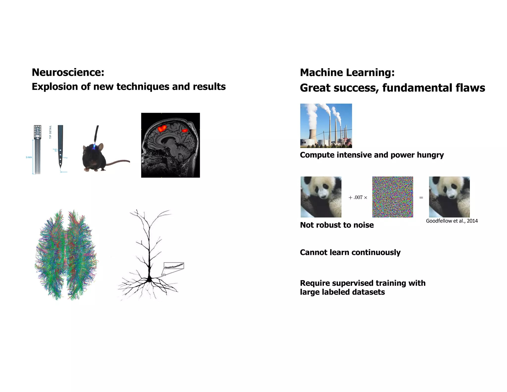
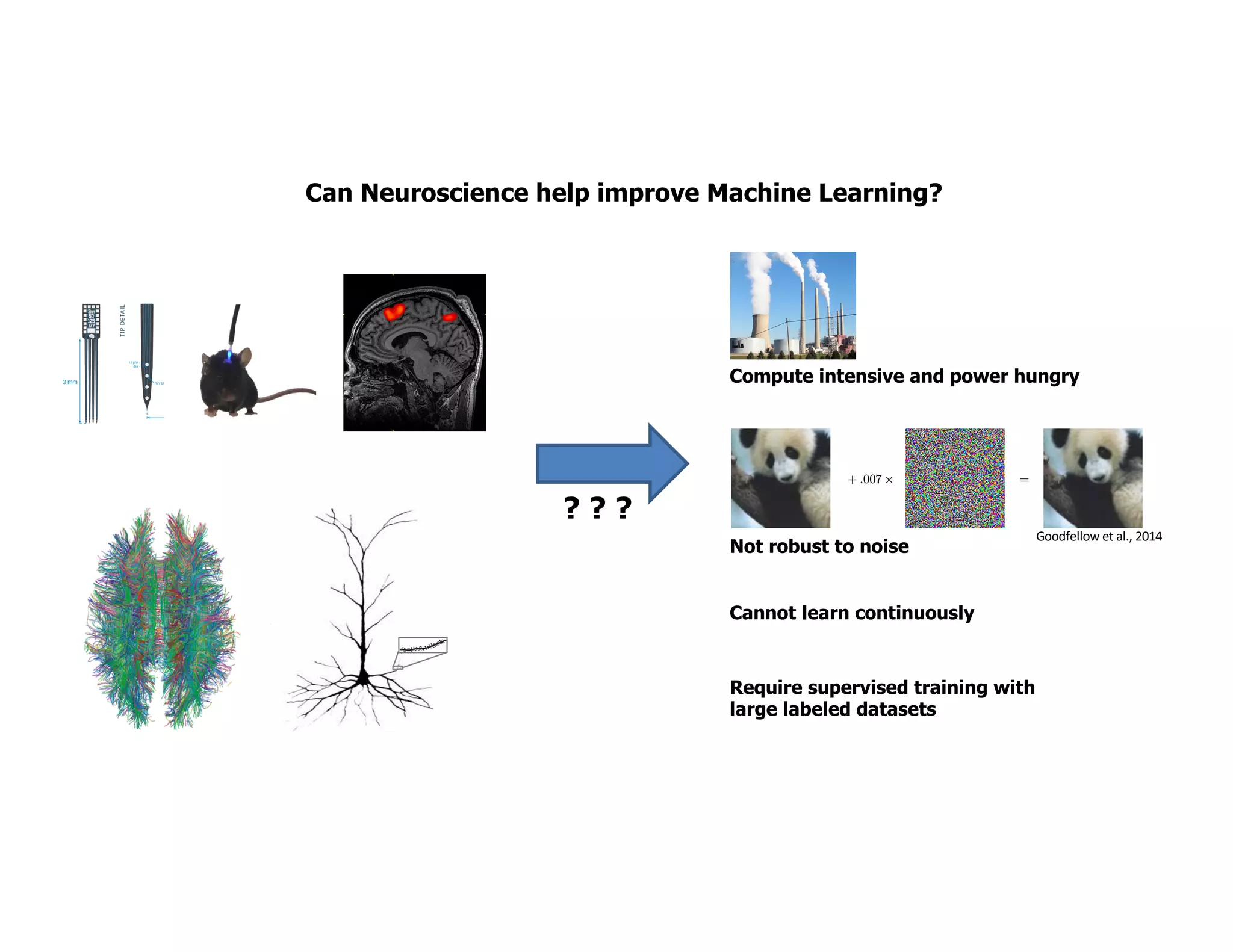
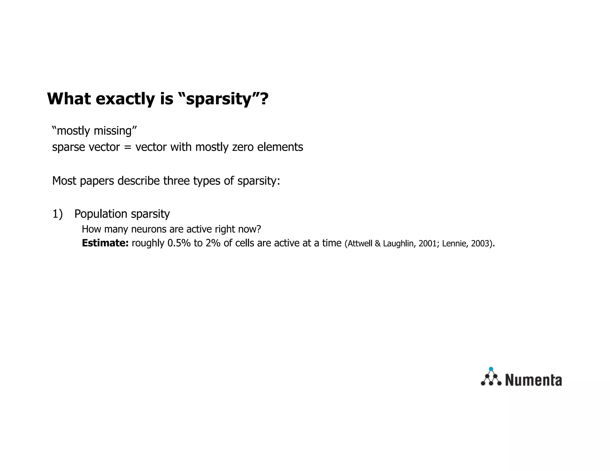
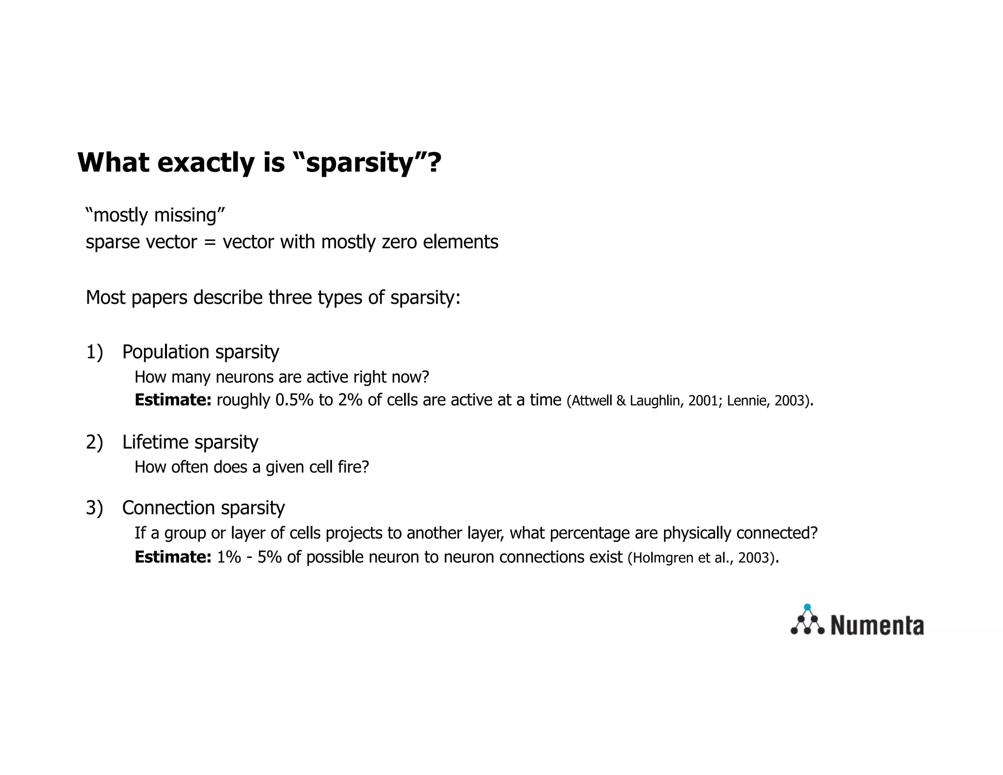
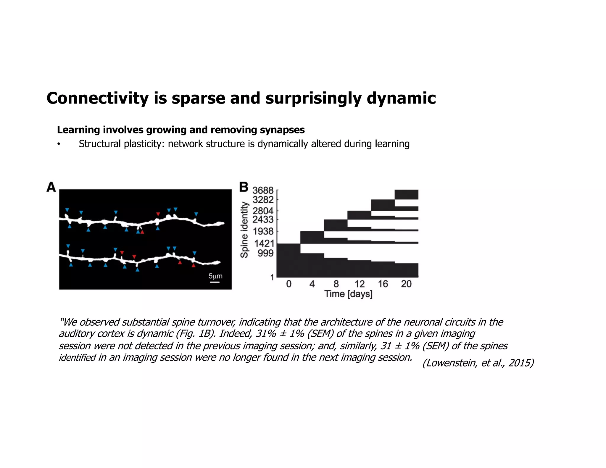
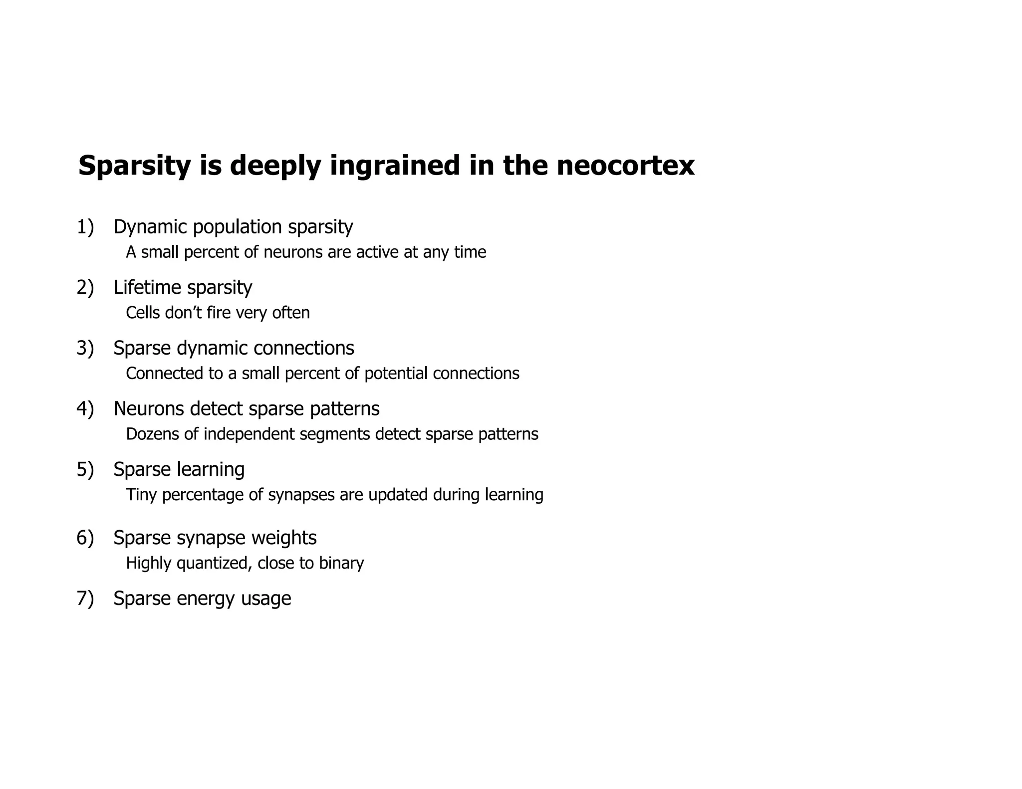
Yale University
Sparsity In The Neocortex,
And Its Implications For Machine Learning
November 18, 2019
Subutai Ahmad
sahmad@numenta.com
@SubutaiAhmad
1) Reverse engineer the neocortex
- biologically accurate theories
- open access neuroscience publications
2) Apply neocortical principles to AI
- improve current techniques
- move toward truly intelligent systems
Mission
Founded in 2005,
by Jeff Hawkins and Donna Dubinsky
Neuroscience:
Explosion of new techniques and results
Machine Learning:
Great success, fundamental flaws
Compute intensive and power hungry
Goodfellow et al., 2014
Not robust to noise
Cannot learn continuously
Require supervised training with
large labeled datasets
Compute intensive and power hungry
Goodfellow et al., 2014
Not robust to noise
Cannot learn continuously
Require supervised training with
large labeled datasets
? ? ?
Can Neuroscience help improve Machine Learning?
Source: Prof. Hasan, Max-Planck-Institute for Research
What exactly is “sparsity”?
“mostly missing”
sparse vector = vector with mostly zero elements
Most papers describe three types of sparsity:
1) Population sparsity
How many neurons are active right now?
Estimate: roughly 0.5% to 2% of cells are active at a time (Attwell & Laughlin, 2001; Lennie, 2003).
Population sparsity changes with learning
Cell Assembly Order
3 4 5 6
Numberofunique
cellassemblies
x104
0
1
2
3
4
5
6
7
Trial Number
0 5 10 15 20ActivationDensity
# 10
-3
3
4
5
6
7
8
9
10
11
12
V1
AL
Subsetindex
0
0.01
0.02
0.03
0.04
AL
D
ataShuffled
Poisson
Subsetindex
0
0.02
0.04
0.06
0.08
V1
Trial 1 Trial 20
Visual
Stimulus
Screen
A
Time (sec)
5 10 15 20 25 30
Neuron#
0
50
100
150
200
250
300
350
Time (sec)
5 10 15 20 25 30
Neuron#
0
50
100
150
200
250
300
350
Time (sec)
5 10 15 20 25 30
Neuron#
0
20
40
60
80
100
120
140
160
Time (sec)
5 10 15 20 25 30
Neuron#
0
20
40
60
80
100
120
140
160
Cell Assembly Order
3 4 5 6
0
500
1000
1500
2000
2500
3000
Data
Shuffled
Poisson
D
ataShuffled
Poisson
ALV1
ALV1
V1
AL
B
C
F
E
D
3-order cell
assembly
single cell
-1 -0.5 0 0.5 1
0
0.1
0.2
0.3
-1 -0.5 0 0.5 1
0
0.02
0.04
0.06
0.08
Time jitter (sec)
Prob.ofobserving
repeatedcellassembly
Time jitter (sec)
Prob.ofobserving
repeatedcellassembly
Spencer L.
Smith
(Stirman et al, 2016)
YiYi Yu
Activity becomes sparser with repeated presentations
Cell Assembly Order
3 4 5 6
Numberofunique
cellassemblies
x104
0
1
2
3
4
5
6
7
Trial Number
0 5 10 15 20
ActivationDensity
3
4
5
6
7
8
9
10
11 V1
AL
Subsetindex
0
0.01
0.02
0.03
0.04
D
ataShuffled
Poisson
Subsetindex
0
0.02
0.04
0.06
0.08
Trial 1 Trial 20
Visual
Stimulus
Screen
Time (sec)
5 10 15 20 25 30
Neuron#
0
50
100
150
200
250
300
350
Time (sec)
5 10 15 20 25 30
Neuron#
0
50
100
150
200
250
300
350
Time (sec)
5 10 15 20 25 30
Neuron#
0
20
40
60
80
100
120
140
160
Time (sec)
5 10 15 20 25 30
Neuron#
0
20
40
60
80
100
120
140
160
Cell Assembly Order
3 4 5 6
0
500
1000
1500
2000
2500
3000
Data
Shuffled
Poisson
D
ataShuffled
Poisson
ALV1
ALV1
V1
AL
3-order cell
assembly
single cell
-1 -0.5 0 0.5 1
0
0.1
0.2
0.3
-1 -0.5 0 0.5 1
0
0.02
0.04
0.06
0.08
Time jitter (sec)
Prob.ofobserving
repeatedcellassembly
Time jitter (sec)
Prob.ofobserving
repeatedcellassembly
Cell Assembly Order
3 4 5 6
Numberofunique
cellassemblies
x104
0
1
2
3
4
5
6
7
Trial Number
0 5 10 15 20
ActivationDensity
# 10-3
3
4
5
6
7
8
9
10
11
12
V1
AL
D
ataShuffled
Poisson
Subsetindex
0
0.02
0.04
0.06
0.08
V1
Trial 1 Trial 20
Visual
Stimulus
Screen
Time (sec)
5 10 15 20 25 30
Neuron#
0
50
100
150
200
250
300
350
Time (sec)
5 10 15 20 25 30
0
50
100
150
200
250
300
350
140
160
140
160
Cel
3
0
500
1000
1500
2000
2500
3000V1
AV1
V1
AL
0.3
0.08
ly
bly
See also (Vinje & Gallant, 2002) Simultaneous wide-field calcium imaging from area V1 and AL in awake mouse
20 presentations of a 30-second natural movie
Population responses in V1 (n=352) and AL (n=163)
Percent active cells drops: from about 1% to 0.4%
What exactly is “sparsity”?
“mostly missing”
sparse vector = vector with mostly zero elements
Most papers describe three types of sparsity:
1) Population sparsity
How many neurons are active right now?
Estimate: roughly 0.5% to 2% of cells are active at a time (Attwell & Laughlin, 2001; Lennie, 2003).
2) Lifetime sparsity
How often does a given cell fire?
3) Connection sparsity
If a group or layer of cells projects to another layer, what percentage are physically connected?
Estimate: 1% - 5% of possible neuron to neuron connections exist (Holmgren et al., 2003).
Connectivity is sparse and surprisingly dynamic
“We observed substantial spine turnover, indicating that the architecture of the neuronal circuits in the
auditory cortex is dynamic (Fig. 1B). Indeed, 31% ± 1% (SEM) of the spines in a given imaging
session were not detected in the previous imaging session; and, similarly, 31 ± 1% (SEM) of the spines
identified in an imaging session were no longer found in the next imaging session.
(Lowenstein, et al., 2015)
Learning involves growing and removing synapses
• Structural plasticity: network structure is dynamically altered during learning
What exactly is “sparsity”?
“mostly missing”
sparse vector = vector with mostly zero elements
Most papers describe three types of sparsity:
1) Population sparsity
How many neurons are active right now?
Estimate: roughly 0.5% to 2% of cells are active at a time (Attwell & Laughlin, 2001; Lennie, 2003).
2) Lifetime sparsity
How often does a given cell fire?
3) Connection sparsity
If a group or layer of cells projects to another layer, what percentage are physically connected?
Estimate: 1% - 5% of possible neuron to neuron connections exist (Holmgren et al., 2003).
…but there’s more to sparsity…
Source: Smirnakis Lab, Baylor College of Medicine
Dendrites of cortical neurons detect sparse patterns
(Mel, 1992; Branco & Häusser, 2011; Schiller et al,
2000; Losonczy, 2006; Antic et al, 2010; Major et al,
2013; Spruston, 2008; Milojkovic et al, 2005, etc.)
Major, Larkum and Schiller 2013
13
Pyramidal neuron
3K to 10K synapses
Dendrites contain dozens of independent computational segments
These segments become active with cluster of 10-20 active synapses
Neurons detect highly sparse patterns, in parallel
Pyramidal neuron
Sparse feedforward patterns
Sparse local patterns
Sparse top-down patterns
14
Learning localized to dendritic segments
“Branch specific plasticity”
If cell becomes active:
• If there was a dendritic spike, reinforce that segment
• If there were no dendritic spikes, grow connections by
subsampling cells active in the past
If cell is not active:
• If there was a dendritic spike, weaken the segments
Sparse learning: only a small part of the neuron is updated
(Gordon et al., 2006; Losonczy et al., 2008; Yang et al., 2014; Cichon & Gang, 2015; El-
Boustani et al., 2018; Weber et al., 2016; Sander et al., 2016; Holthoff et al., 2004)
Sparsity is deeply ingrained in the neocortex
1) Dynamic population sparsity
A small percent of neurons are active at any time
2) Lifetime sparsity
Cells don’t fire very often
3) Sparse dynamic connections
Connected to a small percent of potential connections
4) Neurons detect sparse patterns
Dozens of independent segments detect sparse patterns
5) Sparse learning
Tiny percentage of synapses are updated during learning
6) Sparse synapse weights
Highly quantized, close to binary
7) Sparse energy usage
On a single neuron, 8-20 synapses on tiny segments of
dendrites can recognize patterns. Thousands of other neurons
send input to it.
How can neurons recognize patterns robustly using a tiny
fraction of available connections and highly sparse activations?
Mathematics of highly sparse representations
Pyramidal neuron
3K to 10K synapses
xi<latexit sha1_base64="(null)">(null)</latexit><latexit sha1_base64="(null)">(null)</latexit><latexit sha1_base64="(null)">(null)</latexit><latexit sha1_base64="(null)">(null)</latexit>
n inputs<latexit sha1_base64="dwl2mcnPQNgv8dEIjD6vL0j60R0=">AAAB+XicbVDLSsNAFJ3UV62vqEtFBovgqiS60GXRjcsW7APaUCbTSTt0MgkzN8USuvQv3LhQxK2bfoc7v8GfcJp2oa0HLhzOuZd77/FjwTU4zpeVW1ldW9/Ibxa2tnd29+z9g7qOEkVZjUYiUk2faCa4ZDXgIFgzVoyEvmANf3A79RtDpjSP5D2MYuaFpCd5wCkBI3VsW+I2sAdIMZdxAnrcsYtOycmAl4k7J8Xy8aT6/XgyqXTsz3Y3oknIJFBBtG65TgxeShRwKti40E40iwkdkB5rGSpJyLSXZpeP8ZlRujiIlCkJOFN/T6Qk1HoU+qYzJNDXi95U/M9rJRBce2n2E5N0tihIBIYIT2PAXa4YBTEyhFDFza2Y9okiFExYBROCu/jyMqlflNzLklM1adygGfLoCJ2ic+SiK1RGd6iCaoiiIXpCL+jVSq1n6816n7XmrPnMIfoD6+MHppeXXg==</latexit>
P(xi · xj ✓)<latexit sha1_base64="(null)">(null)</latexit><latexit sha1_base64="(null)">(null)</latexit><latexit sha1_base64="(null)">(null)</latexit><latexit sha1_base64="(null)">(null)</latexit><latexit sha1_base64="(null)">(null)</latexit><latexit sha1_base64="(null)">(null)</latexit><latexit sha1_base64="(null)">(null)</latexit><latexit sha1_base64="(null)">(null)</latexit><latexit sha1_base64="(null)">(null)</latexit><latexit sha1_base64="(null)">(null)</latexit><latexit sha1_base64="(null)">(null)</latexit><latexit sha1_base64="(null)">(null)</latexit><latexit sha1_base64="(null)">(null)</latexit>
Binary sparse vector matching
= connections on dendrite
= input activity
We can get excellent stability and robustness
by reducing , at the cost of increased “false
positives” and interference.
Can compute the probability of a random
vector matching a given :
Numerator: volume around point (white)
Denominator: full volume of space (grey)
P (xi · xj ✓) =
P|xi|
b=✓ | ⌦n
(xi, b, |xj|) |
n
|xj |<latexit sha1_base64="(null)">(null)</latexit><latexit sha1_base64="(null)">(null)</latexit><latexit sha1_base64="(null)">(null)</latexit><latexit sha1_base64="(null)">(null)</latexit>
|⌦n
(xi, b, k)| =
✓
|xi|
b
◆✓
n |xi|
k b
◆
<latexit sha1_base64="(null)">(null)</latexit><latexit sha1_base64="(null)">(null)</latexit><latexit sha1_base64="(null)">(null)</latexit><latexit sha1_base64="(null)">(null)</latexit>
xi<latexit sha1_base64="(null)">(null)</latexit><latexit sha1_base64="(null)">(null)</latexit><latexit sha1_base64="(null)">(null)</latexit><latexit sha1_base64="(null)">(null)</latexit>
P(xi · xj ✓)<latexit sha1_base64="(null)">(null)</latexit><latexit sha1_base64="(null)">(null)</latexit><latexit sha1_base64="(null)">(null)</latexit><latexit sha1_base64="(null)">(null)</latexit><latexit sha1_base64="(null)">(null)</latexit><latexit sha1_base64="(null)">(null)</latexit><latexit sha1_base64="(null)">(null)</latexit><latexit sha1_base64="(null)">(null)</latexit><latexit sha1_base64="(null)">(null)</latexit><latexit sha1_base64="(null)">(null)</latexit><latexit sha1_base64="(null)">(null)</latexit><latexit sha1_base64="(null)">(null)</latexit><latexit sha1_base64="(null)">(null)</latexit>
Sparse high dimensional representations are highly robust
19
1) False positive error decreases exponentially with dimensionality with sparsity.
2) Error rates do not decrease when activity is dense (a=n/2).
3) Assume uniform random distribution of vectors.
Sparse binary vectors: probability of interference Sparse scalar vectors: probability of interference
Standard deep learning layer
A simple differentiable sparse layer
(Hawkins, Ahmad, & Dubinsky, 2011)
(Makhzani & Frey, 2015)
(Ahmad & Scheinkman, 2019)
Outputs of top-k units are maintained,
the rest are set to 0. Just like ReLU, but
with dynamic threshold.
Weight matrix is sparse (most weights
are zero).
1) An exponential boosting term favors units with low activation frequency:
This helps maximize the overall entropy of the layer.
2) Easy extension to sparse convolutional layer
Results: MNIST with sparse networks
1) Networks used CNN layers + one (sparse) linear layer + one softmax output layer.
2) State of the art test set accuracy is between 98.3% and 99.4% (without data
augmentation)
MNIST
MNIST: Accuracy vs noise
(LeCun et al., 1988)
(Ahmad & Scheinkman, 2019)
Sparse networks are significantly better on noisy data
Results: CIFAR-10
DenseNet
• DenseNet (Huang et al., 2016), implements dense level skipping in blocks.
• NotSoDenseNet: sparse transition layers and sparse linear classification layer.
VGG
• VGG19 as in (Simonyan & Zisserman, 2014), with batch norm
• Sparse CNN layers with sparse weights, no linear layer
Results: Google Speech Commands Dataset
Dataset of spoken one word commands
• Released by Google in 2017
• 65,000 utterances, thousands of individuals
• Harder than MNIST
• State of the art is around 95 - 97.5% for 10 categories
• Tested accuracy with white noise
1) Networks used two sparse CNN layers + one sparse linear layer + one softmax output layer.
2) Batchnorm used for all hidden layers
3) Audio files were converted to 32-MFCC coefficients, with data augmentation during training.
28
Continuous learning with active dendrites
Pyramidal neuron
Sparse feedforward patterns
Sparse top-down patterns
Sparse local patterns
29
(Hawkins & Ahmad, 2016)
Continuous learning with active dendrites
Model pyramidal neuron
Simple localized learning rules
When a cell becomes active:
1) If a segment detected pattern, reinforce that segment
2) If no segment detected a pattern, grow new connections
on new dendritic segment
If cell did not become active:
1) If a segment detected pattern, weaken that segment
- Learning consists of growing new connections
- Neurons learn continuously but since patterns are
sparse, new patterns don’t interfere with old ones
Sparse top-down context
Sparse local context
Sparse feedforward patterns
30
(Hawkins & Ahmad, 2016)
Recurrent layer forms an unsupervised predictive system
Model pyramidal neuron
Sparse top-down context
Sparse local context
Sparse feedforward patterns
1) Associates past activity as context for current activity
2) Automatically learns from prediction errors
3) Learns continuously without forgetting past patterns
4) Can learn complex high-Markov order sequences
Recurrent
Neural network
(ESN, LSTM)
HTM*
31
Continuous learning with streaming data sources
(Cui et al, Neural Computation, Nov 2016) HTM = Hierarchical Temporal Memory
2015-04-20
Monday
2015-04-21
Tuesday
2015-04-22
Wednesday
2015-04-23
Thursday
2015-04-24
Friday
2015-04-25
Saturday
2015-04-26
Sunday
0 k
5 k
10 k
15 k
20 k
25 k
30 k
PassengerCountin30minwindow
A
B C
Shift
ARIM
ALSTM
1000LSTM
3000LSTM
6000
TM
0.0
0.2
0.4
0.6
0.8
1.0
NRMSE
0.00
0.05
0.10
0.15
0.20
0.25
0.30
0.35
MAPE
0.0
0.5
1.0
1.5
2.0
2.5
NegativeLog-likelihood
Shift
ARIM
ALSTM
1000LSTM
3000LSTM
6000
TM
LSTM
1000LSTM
3000LSTM
6000
TM
D
NYC Taxi demand datastream
Source: http://www.nyc.gov/html/tlc/html/about/trip_record_data.shtml
?
Apr01
15
Apr08
15
Apr15
15
Apr22
15
Apr29
15
M
ay
06
15
LSTM6000
HTMMeanabsolutepercenterror
0.06
0.08
0.10
0.12
0.14
Dynamics of pattern changed
32(Cui et al, Neural Computation, 2016)
Adapts quickly to changing statistics
• Sparse connections
CNN
Implications of sparsity for machine learning
• Sparse connections
• Sparse activations
Improved robustness
no loss of accuracy
Large performance
gains on hardware
energy – speed – size
• Compartmental neurons
(aka active dendrites)
Continuous learning
quickly reacts to
changes
• Intralaminar circuits
Unsupervised learning
predictive learning
without teacher signal
CNN
Point neuron
Neuroscience principles inform each of these steps
Need to design hardware architectures that exploit these properties
Implications of sparsity for machine learning
• Sparse connections
• Sparse activations
Improved robustness
• Compartmental neurons
(aka active dendrites)
Continuous learning
• Intralaminar circuits
Unsupervised learning
• Multilaminar circuits
- Reference frames
- Sensory-motor
3D Object models
Intelligent Robotics
Point neuron
From sparsity to general intelligence
Implications for hardware architectures
1) Population sparsity
2) Lifetime sparsity
3) Sparse dynamic connections
4) Neurons detect sparse patterns
5) Sparse learning
6) Highly quantized synapse weights
7) Sparse energy usage

Sparsity In The Neocortex, And Its Implications For Machine Learning

  • 1.
    Yale University Sparsity InThe Neocortex, And Its Implications For Machine Learning November 18, 2019 Subutai Ahmad sahmad@numenta.com @SubutaiAhmad
  • 2.
    1) Reverse engineerthe neocortex - biologically accurate theories - open access neuroscience publications 2) Apply neocortical principles to AI - improve current techniques - move toward truly intelligent systems Mission Founded in 2005, by Jeff Hawkins and Donna Dubinsky
  • 3.
    Neuroscience: Explosion of newtechniques and results Machine Learning: Great success, fundamental flaws Compute intensive and power hungry Goodfellow et al., 2014 Not robust to noise Cannot learn continuously Require supervised training with large labeled datasets
  • 4.
    Compute intensive andpower hungry Goodfellow et al., 2014 Not robust to noise Cannot learn continuously Require supervised training with large labeled datasets ? ? ? Can Neuroscience help improve Machine Learning?
  • 5.
    Source: Prof. Hasan,Max-Planck-Institute for Research
  • 6.
    What exactly is“sparsity”? “mostly missing” sparse vector = vector with mostly zero elements Most papers describe three types of sparsity: 1) Population sparsity How many neurons are active right now? Estimate: roughly 0.5% to 2% of cells are active at a time (Attwell & Laughlin, 2001; Lennie, 2003).
  • 7.
    Population sparsity changeswith learning Cell Assembly Order 3 4 5 6 Numberofunique cellassemblies x104 0 1 2 3 4 5 6 7 Trial Number 0 5 10 15 20ActivationDensity # 10 -3 3 4 5 6 7 8 9 10 11 12 V1 AL Subsetindex 0 0.01 0.02 0.03 0.04 AL D ataShuffled Poisson Subsetindex 0 0.02 0.04 0.06 0.08 V1 Trial 1 Trial 20 Visual Stimulus Screen A Time (sec) 5 10 15 20 25 30 Neuron# 0 50 100 150 200 250 300 350 Time (sec) 5 10 15 20 25 30 Neuron# 0 50 100 150 200 250 300 350 Time (sec) 5 10 15 20 25 30 Neuron# 0 20 40 60 80 100 120 140 160 Time (sec) 5 10 15 20 25 30 Neuron# 0 20 40 60 80 100 120 140 160 Cell Assembly Order 3 4 5 6 0 500 1000 1500 2000 2500 3000 Data Shuffled Poisson D ataShuffled Poisson ALV1 ALV1 V1 AL B C F E D 3-order cell assembly single cell -1 -0.5 0 0.5 1 0 0.1 0.2 0.3 -1 -0.5 0 0.5 1 0 0.02 0.04 0.06 0.08 Time jitter (sec) Prob.ofobserving repeatedcellassembly Time jitter (sec) Prob.ofobserving repeatedcellassembly Spencer L. Smith (Stirman et al, 2016) YiYi Yu
  • 8.
    Activity becomes sparserwith repeated presentations Cell Assembly Order 3 4 5 6 Numberofunique cellassemblies x104 0 1 2 3 4 5 6 7 Trial Number 0 5 10 15 20 ActivationDensity 3 4 5 6 7 8 9 10 11 V1 AL Subsetindex 0 0.01 0.02 0.03 0.04 D ataShuffled Poisson Subsetindex 0 0.02 0.04 0.06 0.08 Trial 1 Trial 20 Visual Stimulus Screen Time (sec) 5 10 15 20 25 30 Neuron# 0 50 100 150 200 250 300 350 Time (sec) 5 10 15 20 25 30 Neuron# 0 50 100 150 200 250 300 350 Time (sec) 5 10 15 20 25 30 Neuron# 0 20 40 60 80 100 120 140 160 Time (sec) 5 10 15 20 25 30 Neuron# 0 20 40 60 80 100 120 140 160 Cell Assembly Order 3 4 5 6 0 500 1000 1500 2000 2500 3000 Data Shuffled Poisson D ataShuffled Poisson ALV1 ALV1 V1 AL 3-order cell assembly single cell -1 -0.5 0 0.5 1 0 0.1 0.2 0.3 -1 -0.5 0 0.5 1 0 0.02 0.04 0.06 0.08 Time jitter (sec) Prob.ofobserving repeatedcellassembly Time jitter (sec) Prob.ofobserving repeatedcellassembly Cell Assembly Order 3 4 5 6 Numberofunique cellassemblies x104 0 1 2 3 4 5 6 7 Trial Number 0 5 10 15 20 ActivationDensity # 10-3 3 4 5 6 7 8 9 10 11 12 V1 AL D ataShuffled Poisson Subsetindex 0 0.02 0.04 0.06 0.08 V1 Trial 1 Trial 20 Visual Stimulus Screen Time (sec) 5 10 15 20 25 30 Neuron# 0 50 100 150 200 250 300 350 Time (sec) 5 10 15 20 25 30 0 50 100 150 200 250 300 350 140 160 140 160 Cel 3 0 500 1000 1500 2000 2500 3000V1 AV1 V1 AL 0.3 0.08 ly bly See also (Vinje & Gallant, 2002) Simultaneous wide-field calcium imaging from area V1 and AL in awake mouse 20 presentations of a 30-second natural movie Population responses in V1 (n=352) and AL (n=163) Percent active cells drops: from about 1% to 0.4%
  • 9.
    What exactly is“sparsity”? “mostly missing” sparse vector = vector with mostly zero elements Most papers describe three types of sparsity: 1) Population sparsity How many neurons are active right now? Estimate: roughly 0.5% to 2% of cells are active at a time (Attwell & Laughlin, 2001; Lennie, 2003). 2) Lifetime sparsity How often does a given cell fire? 3) Connection sparsity If a group or layer of cells projects to another layer, what percentage are physically connected? Estimate: 1% - 5% of possible neuron to neuron connections exist (Holmgren et al., 2003).
  • 10.
    Connectivity is sparseand surprisingly dynamic “We observed substantial spine turnover, indicating that the architecture of the neuronal circuits in the auditory cortex is dynamic (Fig. 1B). Indeed, 31% ± 1% (SEM) of the spines in a given imaging session were not detected in the previous imaging session; and, similarly, 31 ± 1% (SEM) of the spines identified in an imaging session were no longer found in the next imaging session. (Lowenstein, et al., 2015) Learning involves growing and removing synapses • Structural plasticity: network structure is dynamically altered during learning
  • 11.
    What exactly is“sparsity”? “mostly missing” sparse vector = vector with mostly zero elements Most papers describe three types of sparsity: 1) Population sparsity How many neurons are active right now? Estimate: roughly 0.5% to 2% of cells are active at a time (Attwell & Laughlin, 2001; Lennie, 2003). 2) Lifetime sparsity How often does a given cell fire? 3) Connection sparsity If a group or layer of cells projects to another layer, what percentage are physically connected? Estimate: 1% - 5% of possible neuron to neuron connections exist (Holmgren et al., 2003). …but there’s more to sparsity…
  • 12.
    Source: Smirnakis Lab,Baylor College of Medicine
  • 13.
    Dendrites of corticalneurons detect sparse patterns (Mel, 1992; Branco & Häusser, 2011; Schiller et al, 2000; Losonczy, 2006; Antic et al, 2010; Major et al, 2013; Spruston, 2008; Milojkovic et al, 2005, etc.) Major, Larkum and Schiller 2013 13 Pyramidal neuron 3K to 10K synapses Dendrites contain dozens of independent computational segments These segments become active with cluster of 10-20 active synapses Neurons detect highly sparse patterns, in parallel
  • 14.
    Pyramidal neuron Sparse feedforwardpatterns Sparse local patterns Sparse top-down patterns 14 Learning localized to dendritic segments “Branch specific plasticity” If cell becomes active: • If there was a dendritic spike, reinforce that segment • If there were no dendritic spikes, grow connections by subsampling cells active in the past If cell is not active: • If there was a dendritic spike, weaken the segments Sparse learning: only a small part of the neuron is updated (Gordon et al., 2006; Losonczy et al., 2008; Yang et al., 2014; Cichon & Gang, 2015; El- Boustani et al., 2018; Weber et al., 2016; Sander et al., 2016; Holthoff et al., 2004)
  • 15.
    Sparsity is deeplyingrained in the neocortex 1) Dynamic population sparsity A small percent of neurons are active at any time 2) Lifetime sparsity Cells don’t fire very often 3) Sparse dynamic connections Connected to a small percent of potential connections 4) Neurons detect sparse patterns Dozens of independent segments detect sparse patterns 5) Sparse learning Tiny percentage of synapses are updated during learning 6) Sparse synapse weights Highly quantized, close to binary 7) Sparse energy usage
  • 17.
    On a singleneuron, 8-20 synapses on tiny segments of dendrites can recognize patterns. Thousands of other neurons send input to it. How can neurons recognize patterns robustly using a tiny fraction of available connections and highly sparse activations? Mathematics of highly sparse representations Pyramidal neuron 3K to 10K synapses xi<latexit sha1_base64="(null)">(null)</latexit><latexit sha1_base64="(null)">(null)</latexit><latexit sha1_base64="(null)">(null)</latexit><latexit sha1_base64="(null)">(null)</latexit> n inputs<latexit sha1_base64="dwl2mcnPQNgv8dEIjD6vL0j60R0=">AAAB+XicbVDLSsNAFJ3UV62vqEtFBovgqiS60GXRjcsW7APaUCbTSTt0MgkzN8USuvQv3LhQxK2bfoc7v8GfcJp2oa0HLhzOuZd77/FjwTU4zpeVW1ldW9/Ibxa2tnd29+z9g7qOEkVZjUYiUk2faCa4ZDXgIFgzVoyEvmANf3A79RtDpjSP5D2MYuaFpCd5wCkBI3VsW+I2sAdIMZdxAnrcsYtOycmAl4k7J8Xy8aT6/XgyqXTsz3Y3oknIJFBBtG65TgxeShRwKti40E40iwkdkB5rGSpJyLSXZpeP8ZlRujiIlCkJOFN/T6Qk1HoU+qYzJNDXi95U/M9rJRBce2n2E5N0tihIBIYIT2PAXa4YBTEyhFDFza2Y9okiFExYBROCu/jyMqlflNzLklM1adygGfLoCJ2ic+SiK1RGd6iCaoiiIXpCL+jVSq1n6816n7XmrPnMIfoD6+MHppeXXg==</latexit> P(xi · xj ✓)<latexit sha1_base64="(null)">(null)</latexit><latexit sha1_base64="(null)">(null)</latexit><latexit sha1_base64="(null)">(null)</latexit><latexit sha1_base64="(null)">(null)</latexit><latexit sha1_base64="(null)">(null)</latexit><latexit sha1_base64="(null)">(null)</latexit><latexit sha1_base64="(null)">(null)</latexit><latexit sha1_base64="(null)">(null)</latexit><latexit sha1_base64="(null)">(null)</latexit><latexit sha1_base64="(null)">(null)</latexit><latexit sha1_base64="(null)">(null)</latexit><latexit sha1_base64="(null)">(null)</latexit><latexit sha1_base64="(null)">(null)</latexit> Binary sparse vector matching = connections on dendrite = input activity
  • 18.
    We can getexcellent stability and robustness by reducing , at the cost of increased “false positives” and interference. Can compute the probability of a random vector matching a given : Numerator: volume around point (white) Denominator: full volume of space (grey) P (xi · xj ✓) = P|xi| b=✓ | ⌦n (xi, b, |xj|) | n |xj |<latexit sha1_base64="(null)">(null)</latexit><latexit sha1_base64="(null)">(null)</latexit><latexit sha1_base64="(null)">(null)</latexit><latexit sha1_base64="(null)">(null)</latexit> |⌦n (xi, b, k)| = ✓ |xi| b ◆✓ n |xi| k b ◆ <latexit sha1_base64="(null)">(null)</latexit><latexit sha1_base64="(null)">(null)</latexit><latexit sha1_base64="(null)">(null)</latexit><latexit sha1_base64="(null)">(null)</latexit> xi<latexit sha1_base64="(null)">(null)</latexit><latexit sha1_base64="(null)">(null)</latexit><latexit sha1_base64="(null)">(null)</latexit><latexit sha1_base64="(null)">(null)</latexit> P(xi · xj ✓)<latexit sha1_base64="(null)">(null)</latexit><latexit sha1_base64="(null)">(null)</latexit><latexit sha1_base64="(null)">(null)</latexit><latexit sha1_base64="(null)">(null)</latexit><latexit sha1_base64="(null)">(null)</latexit><latexit sha1_base64="(null)">(null)</latexit><latexit sha1_base64="(null)">(null)</latexit><latexit sha1_base64="(null)">(null)</latexit><latexit sha1_base64="(null)">(null)</latexit><latexit sha1_base64="(null)">(null)</latexit><latexit sha1_base64="(null)">(null)</latexit><latexit sha1_base64="(null)">(null)</latexit><latexit sha1_base64="(null)">(null)</latexit> Sparse high dimensional representations are highly robust
  • 19.
    Sparse high dimensionalrepresentations are highly robust 19 1) False positive error decreases exponentially with dimensionality with sparsity. 2) Error rates do not decrease when activity is dense (a=n/2). 3) Assume uniform random distribution of vectors. Sparse binary vectors: probability of interference Sparse scalar vectors: probability of interference
  • 20.
  • 21.
    A simple differentiablesparse layer (Hawkins, Ahmad, & Dubinsky, 2011) (Makhzani & Frey, 2015) (Ahmad & Scheinkman, 2019) Outputs of top-k units are maintained, the rest are set to 0. Just like ReLU, but with dynamic threshold. Weight matrix is sparse (most weights are zero). 1) An exponential boosting term favors units with low activation frequency: This helps maximize the overall entropy of the layer. 2) Easy extension to sparse convolutional layer
  • 22.
    Results: MNIST withsparse networks 1) Networks used CNN layers + one (sparse) linear layer + one softmax output layer. 2) State of the art test set accuracy is between 98.3% and 99.4% (without data augmentation) MNIST MNIST: Accuracy vs noise (LeCun et al., 1988) (Ahmad & Scheinkman, 2019)
  • 23.
    Sparse networks aresignificantly better on noisy data
  • 24.
    Sparse networks aresignificantly better on noisy data
  • 25.
    Sparse networks aresignificantly better on noisy data
  • 26.
    Results: CIFAR-10 DenseNet • DenseNet(Huang et al., 2016), implements dense level skipping in blocks. • NotSoDenseNet: sparse transition layers and sparse linear classification layer. VGG • VGG19 as in (Simonyan & Zisserman, 2014), with batch norm • Sparse CNN layers with sparse weights, no linear layer
  • 27.
    Results: Google SpeechCommands Dataset Dataset of spoken one word commands • Released by Google in 2017 • 65,000 utterances, thousands of individuals • Harder than MNIST • State of the art is around 95 - 97.5% for 10 categories • Tested accuracy with white noise 1) Networks used two sparse CNN layers + one sparse linear layer + one softmax output layer. 2) Batchnorm used for all hidden layers 3) Audio files were converted to 32-MFCC coefficients, with data augmentation during training.
  • 28.
    28 Continuous learning withactive dendrites Pyramidal neuron Sparse feedforward patterns Sparse top-down patterns Sparse local patterns
  • 29.
    29 (Hawkins & Ahmad,2016) Continuous learning with active dendrites Model pyramidal neuron Simple localized learning rules When a cell becomes active: 1) If a segment detected pattern, reinforce that segment 2) If no segment detected a pattern, grow new connections on new dendritic segment If cell did not become active: 1) If a segment detected pattern, weaken that segment - Learning consists of growing new connections - Neurons learn continuously but since patterns are sparse, new patterns don’t interfere with old ones Sparse top-down context Sparse local context Sparse feedforward patterns
  • 30.
    30 (Hawkins & Ahmad,2016) Recurrent layer forms an unsupervised predictive system Model pyramidal neuron Sparse top-down context Sparse local context Sparse feedforward patterns 1) Associates past activity as context for current activity 2) Automatically learns from prediction errors 3) Learns continuously without forgetting past patterns 4) Can learn complex high-Markov order sequences
  • 31.
    Recurrent Neural network (ESN, LSTM) HTM* 31 Continuouslearning with streaming data sources (Cui et al, Neural Computation, Nov 2016) HTM = Hierarchical Temporal Memory 2015-04-20 Monday 2015-04-21 Tuesday 2015-04-22 Wednesday 2015-04-23 Thursday 2015-04-24 Friday 2015-04-25 Saturday 2015-04-26 Sunday 0 k 5 k 10 k 15 k 20 k 25 k 30 k PassengerCountin30minwindow A B C Shift ARIM ALSTM 1000LSTM 3000LSTM 6000 TM 0.0 0.2 0.4 0.6 0.8 1.0 NRMSE 0.00 0.05 0.10 0.15 0.20 0.25 0.30 0.35 MAPE 0.0 0.5 1.0 1.5 2.0 2.5 NegativeLog-likelihood Shift ARIM ALSTM 1000LSTM 3000LSTM 6000 TM LSTM 1000LSTM 3000LSTM 6000 TM D NYC Taxi demand datastream Source: http://www.nyc.gov/html/tlc/html/about/trip_record_data.shtml ?
  • 32.
  • 33.
    • Sparse connections CNN Implicationsof sparsity for machine learning
  • 34.
    • Sparse connections •Sparse activations Improved robustness no loss of accuracy Large performance gains on hardware energy – speed – size • Compartmental neurons (aka active dendrites) Continuous learning quickly reacts to changes • Intralaminar circuits Unsupervised learning predictive learning without teacher signal CNN Point neuron Neuroscience principles inform each of these steps Need to design hardware architectures that exploit these properties Implications of sparsity for machine learning
  • 36.
    • Sparse connections •Sparse activations Improved robustness • Compartmental neurons (aka active dendrites) Continuous learning • Intralaminar circuits Unsupervised learning • Multilaminar circuits - Reference frames - Sensory-motor 3D Object models Intelligent Robotics Point neuron From sparsity to general intelligence
  • 37.
    Implications for hardwarearchitectures 1) Population sparsity 2) Lifetime sparsity 3) Sparse dynamic connections 4) Neurons detect sparse patterns 5) Sparse learning 6) Highly quantized synapse weights 7) Sparse energy usage