Sorting
Prof.Kalyani N. Neve
GHRIBM,Jalgaon
2/6/2019 Kalyani N Neve 1
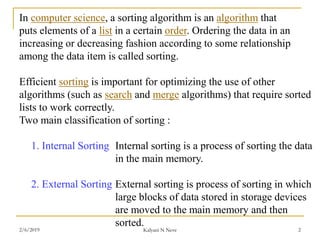
In computer science, a sorting algorithm is an algorithm that
puts elements of a list in a certain order. Ordering the data in an
increasing or decreasing fashion according to some relationship
among the data item is called sorting.
Efficient sorting is important for optimizing the use of other
algorithms (such as search and merge algorithms) that require sorted
lists to work correctly.
Two main classification of sorting :
1. Internal Sorting Internal sorting is a process of sorting the data
in the main memory.
2. External Sorting External sorting is process of sorting in which
large blocks of data stored in storage devices
are moved to the main memory and then
sorted.
2/6/2019 Kalyani N Neve 2
1.Insertion Sort :
Suppose an array A with n elements A[1], A[2],…..,A[n] is in
memory. The insertion sort algorithm. Scans A from A[1] to A[n],
inserting each element A[K] into its proper position in the
previously sorted sub array A[1], A[2], …,A[K-1]. That is:
Pass 1: A[1] by itself is trivially sorted.
Pass 2: A[2] is inserted either before or after A[1] so that A[1], A[2]
is sorted.
Pass 3: A[3] is inserted into its proper place in A[1], A[2], that is
before A[1], between A[1] and A[2], or after A[2], So that
A[1], A[2],A[3] is sorted.
2/6/2019 Kalyani N Neve 3
Pass 4: A[4] is inserted into its proper place in A[1],A[2],A[3]
so that:
A[1],A[2],A[3],A[4] is sorted.
.
.
.
.
.
Pass N : A[N] is inserted into its proper place in
A[1],A[2],…,A[N-1] so that :
A[1],A[2],……,A[N] is sorted.
2/6/2019 Kalyani N Neve 4
Algorithm :
INSERTION(A,N)
1. Set A[0] := -∞ [Initializes element]
2. Repeat Steps 3 to 5 for K = 2,3,…..,N:
3. Set TEMP := A[K] and PTR := K-1
4. Repeat while TEMP < A[PTR]:
1. Set A[PTR + 1] := A[PTR]. [Moves element
forward.]
2. Set PTR := PTR – 1
5. Set A[PTR + 1] := TEMP [Inserts element in proper
place.]
[End of Step 2 loop.]
6. Return
2/6/2019 Kalyani N Neve 5
Pass A[0] A[1] A[2] A[3] A[4] A[5] A[6] A[7] A[8]
K=1: -∞ 33 44 11 88 22 66 55
K=2: -∞ 77 33 44 11 88 22 66 55
K=3: -∞ 33 77 44 11 88 22 66 55
K=4: -∞ 33 44 77 11 88 22 66 55
K=5: -∞ 11 33 44 77 88 22 66 55
K=6: -∞ 11 33 44 77 88 22 66 55
K=7: -∞ 11 22 33 44 77 88 66 55
K=8: -∞ 11 22 33 44 66 77 88 55
Sorted: -∞ 11 22 33 44 55 66 77 88
Array A is, 77, 33, 44, 11, 88, 22, 66, 55
77
2/6/2019 Kalyani N Neve 6
2. Selection Sort :
Suppose an array A with n elements A[1], A[2],…..,A[n] is in
memory. The selection sort algo. For sorting A as follows:
Pass 1: Find the location LOC of the smallest in the list of N elements
A[1],A[2],….,A[N], and then interchange A[LOC] and A[1],
Then : A[1] is sorted.
Pass 2: Find the location LOC of the smallest in the sublist of N-1
elements A[1],A[2],….,A[N], and then interchange A[LOC]
and A[2], Then : A[1], A[2]is sorted. Since A[1] <= A[2].
Pass 3:Find the location LOC of the smallest in the sub list of N-2
elements A[1],A[2],….,A[N], and then interchange A[LOC]
and A[3], Then : A[1], A[2],A[3]is sorted. Since A[2] <= A[3].
2/6/2019 Kalyani N Neve 7
.
.
.
Pass N-1:Find the location LOC of the smaller of the elements
A[N-1],A[N], and then interchange A[LOC] and A[N-
1], Then : A[1],A[2],….A[N]is sorted.
Since A[N-1] <= A[N].
Thus A is sorted after N-1 passes.
2/6/2019 Kalyani N Neve 8
Algorithm :
SELECTION(A,N)
1. Repeat Steps 2 and 3 for K=1,2,….,N-1
2. Call Min (A,K,N,LOC)
3. [Interchange A[K] and A[LOC]]
Set TEMP := A[K], A[K] := A{LOC] and A[LOC] :=
TEMP
[End of step 1 loop]
4. Exit
MIN(A,K,N,LOC)
1. Set MIN := A[K] and LOC := K. [Initialize pointers]
2. Repeat for J=K+1,K+2,….,N
If MIN > A[J], then :
Set MIN := A[J] and LOC := A[J] and LOC := J
[End of loop]
3. Return
2/6/2019 Kalyani N Neve 9
Pass A[1] A[2] A[3] A[4] A[5] A[6] A[7] A[8]
K=1:
LOC=4
33 44 11 88 22 66 55
K=2:
LOC=6
11 33 44 77 88 22 66 55
K=3:
LOC=6
11 22 44 77 88 33 66 55
K=4:
LOC=6
11 22 33 77 88 44 66 55
K=5:
LOC=8
11 22 33 44 88 77 66 55
K=6:
LOC=7
11 22 33 44 55 77 66 88
K=7:
LOC=7
11 22 33 44 55 66 77 88
Sorted: 11 22 33 44 55 66 77 88
Array A is, 77, 33, 44, 11, 88, 22, 66, 55
77
2/6/2019 Kalyani N Neve 10
3. Bubble Sort :
Suppose an array A with n elements A[1], A[2],…..,A[n] is in
memory. The bubble sort algo. For sorting A as follows:
Step 1: Compare A[1] and A[2] and arrange them in the desired
order, so that A[1] < A[2]. Then compare A[2] and A[3] and
arrange them so that A[2] < A[3]. Continue until we compare
A[N-1] with A[N] and arrange them.
Step 2: Repeat step 1 with one less comparison, that is, now we
stop after we compare and possibly rearrange A[N-1] and A[N-1].
.
.
.
2/6/2019 Kalyani N Neve 11
Step N-1 : Compare A[1] with A[2] and arrange them so that
A[1] < A[2].
After N-1 steps, the list will be sorted in increasing order.
Suppose the following numbers are sorted in an array A :
32, 51, 27,85, 66, 23, 13, 57
We apply the bubble sort to the array A.
2/6/2019 Kalyani N Neve 12
BUBBLE(DATA, N)
Here DATA is an array with N elements. This algorithm sorts the
elements in DATA.
1. Repeat steps 2 and 3 for K = 1 to N-1.
2. Set PTR := 1. [ Initialize pass pointer PTR]
3. Repeat while PTR <= N – K: [Execute pass]
1. If DATA[PTR] > DATA[PTR + 1], then :
Interchange DATA[PTR] and DATA[PTR + 1]
[End of If structure]
2. Set PTR := PTR + 1.
[End of inner loop]
[End of step 1 outer loop]
4. Exit
2/6/2019 Kalyani N Neve 13
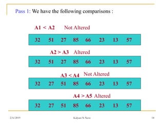
Pass 1: We have the following comparisons :
32 51 27 85 66 23 13 57
32 51 27 85 66 23 13 57
32 27 51 85 66 23 13 57
32 27 51 85 66 23 13 57
A1 A2<
>A2 A3
<A3 A4
A4 A5>
Not Altered
Altered
Not Altered
Altered
2/6/2019 Kalyani N Neve 14
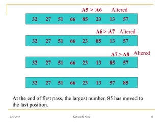
32 27 51 66 85 23 13 57
32 27 51 66 23 85 13 57
32 27 51 66 23 13 85 57
32 27 51 66 23 13 57 85
A5 A6>
>A6 A7
>A7 A8
Altered
Altered
Altered
At the end of first pass, the largest number, 85 has moved to
the last position.
2/6/2019 Kalyani N Neve 15
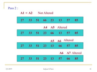
Pass 2 :
27 33 51 66 23 13 57 85
27 33 51 23 66 13 57 85
27 33 51 23 13 66 57 85
27 33 51 23 13 57 66 85
A1 A2<
A4 A5
A5 A6
A6 A7
Not Altered
Altered
Altered
Altered
2/6/2019 Kalyani N Neve 16
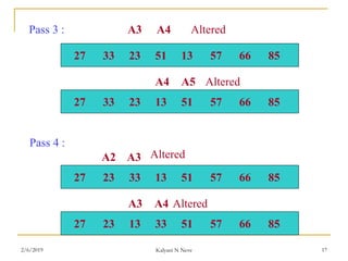
Pass 3 :
27 33 23 51 13 57 66 85
27 33 23 13 51 57 66 85
27 23 33 13 51 57 66 85
27 23 13 33 51 57 66 85
A3 A4
A4 A5
A2 A3
A3 A4
Altered
Altered
Altered
Altered
Pass 4 :
2/6/2019 Kalyani N Neve 17
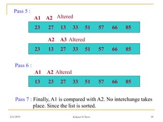
23 27 13 33 51 57 66 85
23 13 27 33 51 57 66 85
A1 A2
A2 A3
Altered
Altered
Pass 5 :
13 23 27 33 51 57 66 85
A1 A2 Altered
Pass 6 :
Pass 7 : Finally, A1 is compared with A2. No interchange takes
place. Since the list is sorted.
2/6/2019 Kalyani N Neve 18
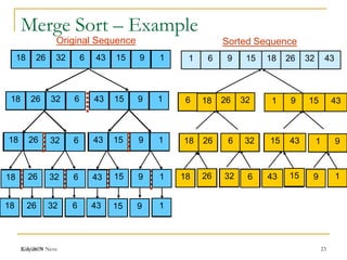
4. Merge Sort :
Suppose an array A with n elements A[1],
A[2],…..,A[n] is in memory. The merge sort algorithm
For sorting A as follows:
2/6/2019 Kalyani N Neve 19
Kalyani N Neve
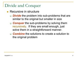
Divide and Conquer
 Recursive in structure
 Divide the problem into sub-problems that are
similar to the original but smaller in size
 Conquer the sub-problems by solving them
recursively. If they are small enough, just
solve them in a straightforward manner.
 Combine the solutions to create a solution to
the original problem
2/6/2019 20
Kalyani N Neve
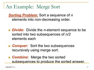
An Example: Merge Sort
Sorting Problem: Sort a sequence of n
elements into non-decreasing order.
 Divide: Divide the n-element sequence to be
sorted into two subsequences of n/2
elements each
 Conquer: Sort the two subsequences
recursively using merge sort.
 Combine: Merge the two sorted
subsequences to produce the sorted answer.
2/6/2019 21
Kalyani N Neve
Merge Sort – Example
18 26 32 6 43 15 9 1
18 26 32 6 43 15 9 1
18 26 32 6 43 15 9 1
2618 632 1543 19
18 26 32 6 43 15 9 1
18 26 32 6 43 15 9 1
18 26 326 15 43 1 9
6 18 26 32 1 9 15 43
1 6 9 15 18 26 32 43
18 26
18 26
18 26
32
32
6
6
32 6
18 26 32 6
43
43
15
15
43 15
9
9
1
1
9 1
43 15 9 1
18 26 32 6 43 15 9 1
18 26 632
626 3218
1543 19
1 915 43
16 9 1518 26 32 43
Original Sequence Sorted Sequence
2/6/2019 23
MERGESORT(LOW, HIGH)
1. Set LOW := 1.
2. If LOW < HIGH: then:
1. Set MID := (LOW + N)/2
2. Call MERGESORT(LOW, MID)
3. Call MERGESORT(MID+1, HIGH)
4. Call MERGE(LOW,MID,HIGH)
[End of step 2 loop]
7. Exit
2/6/2019 Kalyani N Neve 24
MERGE(A, LOW, MID, HIGH)
This algorithm merges two sorted sub arrays into one
array.
1. [Initialize]
h := LOW, i := LOW, j := MID + 1
2. Repeat while h <= MID && j <= HIGH:
If A[h] <= A[j] then:
Set b[i] := A[h]
Set h := h +1
ELSE:
Set b[i] := A[j]
Set j := j +1
[End of If structure]
Set i := i + 1
[End of loop]
2/6/2019 Kalyani N Neve 25
3. If h > MID then:
Set k := j
Repeat while k <= HIGH
Set h[i] := A[k]
Set i := i + 1
ELSE
Set k := h
Repeat while k <= MID
b[i] := a[k];
I := i+1;
4. Set k := LOW
Repeat while k <= HIGH
a[k] := b[k];
5. Return
2/6/2019 Kalyani N Neve 26
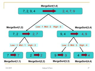
7 7 2 2 9 9 4 4
Low : 1 Mid : 2 High : 4
Low : 1 Mid : 1 High : 2 Low : 3 Mid : 3 High : 4
7, 2, 9, 4 2, 4, 7, 9
2, 77, 2 9, 4 4, 9
MergeSort(1,2)
MergeSort(1,1) MergeSort(2,2)
MergeSort(1,4)
MergeSort(3,4)
MergeSort(3,3) MergeSort(4,4)
2/6/2019 Kalyani N Neve 27
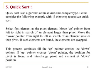
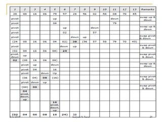
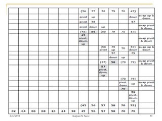
5. Quick Sort :
Quick sort is an algorithm of the divide-and-conquer type. Let us
consider the following example with 13 elements to analyze quick
sort:
Select first element as the pivot element. Move ‘up’ pointer from
left to right in search of an element larger than pivot. Move the
‘down’ pointer from right to left in search of an element smaller
than pivot. If such elements are found, the elements are swapped.
This process continues till the ‘up’ pointer crosses the ‘down’
pointer. If ‘up’ pointer crosses ‘down’ pointer, the position for
pivot is found and interchange pivot and element at ‘down’
position.
2/6/2019 Kalyani N Neve 28
2/6/2019 Kalyani N Neve 29
2/6/2019 Kalyani N Neve 30
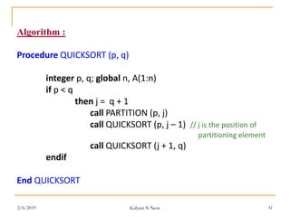
Algorithm :
Procedure QUICKSORT (p, q)
integer p, q; global n, A(1:n)
if p < q
then j = q + 1
call PARTITION (p, j)
call QUICKSORT (p, j – 1) // j is the position of
partitioning element
call QUICKSORT (j + 1, q)
endif
End QUICKSORT
2/6/2019 Kalyani N Neve 31
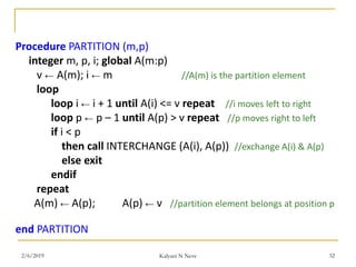
Procedure PARTITION (m,p)
integer m, p, i; global A(m:p)
v ← A(m); i ← m //A(m) is the partition element
loop
loop i ← i + 1 until A(i) <= v repeat //i moves left to right
loop p ← p – 1 until A(p) > v repeat //p moves right to left
if i < p
then call INTERCHANGE (A(i), A(p)) //exchange A(i) & A(p)
else exit
endif
repeat
A(m) ← A(p); A(p) ← v //partition element belongs at position p
end PARTITION
2/6/2019 Kalyani N Neve 32
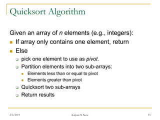
Quicksort Algorithm
Given an array of n elements (e.g., integers):
 If array only contains one element, return
 Else
 pick one element to use as pivot.
 Partition elements into two sub-arrays:
 Elements less than or equal to pivot
 Elements greater than pivot
 Quicksort two sub-arrays
 Return results
2/6/2019 Kalyani N Neve 33
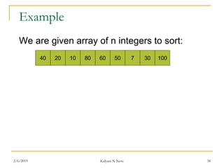
Example
We are given array of n integers to sort:
40 20 10 80 60 50 7 30 100
2/6/2019 Kalyani N Neve 34
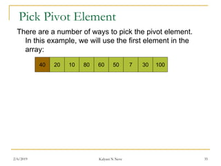
Pick Pivot Element
There are a number of ways to pick the pivot element.
In this example, we will use the first element in the
array:
40 20 10 80 60 50 7 30 100
2/6/2019 Kalyani N Neve 35
Partitioning Array
Given a pivot, partition the elements of the array
such that the resulting array consists of:
1. One sub-array that contains elements >= pivot
2. Another sub-array that contains elements < pivot
The sub-arrays are stored in the original data
array.
Partitioning loops through, swapping elements
below/above pivot.
2/6/2019 Kalyani N Neve 36
40 20 10 80 60 50 7 30 100pivot_index = 0
[0] [1] [2] [3] [4] [5] [6] [7] [8]
i j
2/6/2019 Kalyani N Neve 37
40 20 10 80 60 50 7 30 100pivot_index = 0
[0] [1] [2] [3] [4] [5] [6] [7] [8]
i j
1. While data[i] <= data[pivot]
++i
2/6/2019 Kalyani N Neve 38
40 20 10 80 60 50 7 30 100pivot_index = 0
[0] [1] [2] [3] [4] [5] [6] [7] [8]
i j
1. While data[i] <= data[pivot]
++i
2/6/2019 Kalyani N Neve 39
40 20 10 80 60 50 7 30 100pivot_index = 0
[0] [1] [2] [3] [4] [5] [6] [7] [8]
i j
1. While data[i] <= data[pivot]
++i
2. While data[j] > data[pivot]
--j
2/6/2019 Kalyani N Neve 40
40 20 10 80 60 50 7 30 100pivot_index = 0
[0] [1] [2] [3] [4] [5] [6] [7] [8]
i j
1. While data[i] <= data[pivot]
++i
2. While data[j] > data[pivot]
--j
2/6/2019 Kalyani N Neve 41
40 20 10 80 60 50 7 30 100pivot_index = 0
[0] [1] [2] [3] [4] [5] [6] [7] [8]
i j
1. While data[i] <= data[pivot]
++i
2. While data[j] > data[pivot]
--j
3. If i < j
swap data[i] and data[j]
2/6/2019 Kalyani N Neve 42
40 20 10 30 60 50 7 80 100pivot_index = 0
i j
1. While data[i] <= data[pivot]
++i
2. While data[j] > data[pivot]
--j
3. If i < j
swap data[i] and data[j]
[0] [1] [2] [3] [4] [5] [6] [7] [8]
2/6/2019 Kalyani N Neve 43
40 20 10 30 60 50 7 80 100pivot_index = 0
i j
1. While data[i] <= data[pivot]
++i
2. While data[j] > data[pivot]
--j
3. If i < j
swap data[i] and data[j]
4. While j > i, go to 1.
[0] [1] [2] [3] [4] [5] [6] [7] [8]
2/6/2019 Kalyani N Neve 44
40 20 10 30 60 50 7 80 100pivot_index = 0
i j
1. While data[i] <= data[pivot]
++i
2. While data[j] > data[pivot]
--j
3. If i < j
swap data[i] and data[j]
4. While j > i, go to 1.
[0] [1] [2] [3] [4] [5] [6] [7] [8]
2/6/2019 Kalyani N Neve 45
40 20 10 30 60 50 7 80 100pivot_index = 0
i j
1. While data[i] <= data[pivot]
++i
2. While data[j] > data[pivot]
--j
3. If i < j
swap data[i] and data[j]
4. While j > i, go to 1.
[0] [1] [2] [3] [4] [5] [6] [7] [8]
2/6/2019 Kalyani N Neve 46
40 20 10 30 60 50 7 80 100pivot_index = 0
i j
1. While data[i] <= data[pivot]
++i
2. While data[j] > data[pivot]
--j
3. If i < j
swap data[i] and data[j]
4. While j > i, go to 1.
[0] [1] [2] [3] [4] [5] [6] [7] [8]
2/6/2019 Kalyani N Neve 47
40 20 10 30 60 50 7 80 100pivot_index = 0
i j
1. While data[i] <= data[pivot]
++i
2. While data[j] > data[pivot]
--j
3. If i < j
swap data[i] and data[j]
4. While j > i, go to 1.
[0] [1] [2] [3] [4] [5] [6] [7] [8]
2/6/2019 Kalyani N Neve 48
40 20 10 30 60 50 7 80 100pivot_index = 0
i j
1. While data[i] <= data[pivot]
++i
2. While data[j] > data[pivot]
--j
3. If i < j
swap data[i] and data[j]
4. While j > i, go to 1.
[0] [1] [2] [3] [4] [5] [6] [7] [8]
2/6/2019 Kalyani N Neve 49
1. While data[i] <= data[pivot]
++i
2. While data[j] > data[pivot]
--j
3. If i < j
swap data[i] and data[j]
4. While j > i, go to 1.
40 20 10 30 7 50 60 80 100pivot_index = 0
i j
[0] [1] [2] [3] [4] [5] [6] [7] [8]
2/6/2019 Kalyani N Neve 50
1. While data[i] <= data[pivot]
++i
2. While data[j] > data[pivot]
--j
3. If i < j
swap data[i] and data[j]
4. While j > i, go to 1.
40 20 10 30 7 50 60 80 100pivot_index = 0
i j
[0] [1] [2] [3] [4] [5] [6] [7] [8]
2/6/2019 Kalyani N Neve 51
1. While data[i] <= data[pivot]
++i
2. While data[j] > data[pivot]
--j
3. If i < j
swap data[i] and data[j]
4. While j > i, go to 1.
40 20 10 30 7 50 60 80 100pivot_index = 0
i j
[0] [1] [2] [3] [4] [5] [6] [7] [8]
2/6/2019 Kalyani N Neve 52
1. While data[i] <= data[pivot]
++i
2. While data[j] > data[pivot]
--j
3. If i < j
swap data[i] and data[j]
4. While j > i, go to 1.
40 20 10 30 7 50 60 80 100pivot_index = 0
i j
[0] [1] [2] [3] [4] [5] [6] [7] [8]
2/6/2019 Kalyani N Neve 53
1. While data[i] <= data[pivot]
++i
2. While data[j] > data[pivot]
--j
3. If i < j
swap data[i] and data[j]
4. While j > i, go to 1.
40 20 10 30 7 50 60 80 100pivot_index = 0
i j
[0] [1] [2] [3] [4] [5] [6] [7] [8]
2/6/2019 Kalyani N Neve 54
1. While data[i] <= data[pivot]
++i
2. While data[j] > data[pivot]
--j
3. If i < j
swap data[i] and data[j]
4. While j > i, go to 1.
40 20 10 30 7 50 60 80 100pivot_index = 0
i j
[0] [1] [2] [3] [4] [5] [6] [7] [8]
2/6/2019 Kalyani N Neve 55
1. While data[i] <= data[pivot]
++i
2. While data[j] > data[pivot]
--j
3. If i < j
swap data[i] and data[j]
4. While j > i, go to 1.
40 20 10 30 7 50 60 80 100pivot_index = 0
i j
[0] [1] [2] [3] [4] [5] [6] [7] [8]
2/6/2019 Kalyani N Neve 56
1. While data[i] <= data[pivot]
++i
2. While data[j] > data[pivot]
--j
3. If i < j
swap data[i] and data[j]
4. While j > i, go to 1.
40 20 10 30 7 50 60 80 100pivot_index = 0
i j
[0] [1] [2] [3] [4] [5] [6] [7] [8]
2/6/2019 Kalyani N Neve 57
1. While data[i] <= data[pivot]
++i
2. While data[j] > data[pivot]
--j
3. If i < j
swap data[i] and data[j]
4. While j > i, go to 1.
40 20 10 30 7 50 60 80 100pivot_index = 0
i j
[0] [1] [2] [3] [4] [5] [6] [7] [8]
2/6/2019 Kalyani N Neve 58
1. While data[i] <= data[pivot]
++i
2. While data[j] > data[pivot]
--j
3. If i < j
swap data[i] and data[j]
4. While j > i, go to 1.
5. Swap data[j] and data[pivot_index]
40 20 10 30 7 50 60 80 100pivot_index = 0
i j
[0] [1] [2] [3] [4] [5] [6] [7] [8]
2/6/2019 Kalyani N Neve 59
1. While data[i] <= data[pivot]
++i
2. While data[j] > data[pivot]
--j
3. If i < j
swap data[i] and data[j]
4. While j > i, go to 1.
5. Swap data[j] and data[pivot_index]
7 20 10 30 40 50 60 80 100pivot_index = 4
i j
[0] [1] [2] [3] [4] [5] [6] [7] [8]
2/6/2019 Kalyani N Neve 60
Partition Result
7 20 10 30 40 50 60 80 100
<= data[pivot] > data[pivot]
[0] [1] [2] [3] [4] [5] [6] [7] [8]
2/6/2019 Kalyani N Neve 61
Recursion: Quicksort Sub-arrays
7 20 10 30 40 50 60 80 100
<= data[pivot] > data[pivot]
[0] [1] [2] [3] [4] [5] [6] [7] [8]
2/6/2019 Kalyani N Neve 62
6. Radix Sort :
Radix sort is a method can be used to sort a list of names
alphabetically. To sort alphabetically radix is 26, the 26 letters of
the alphabet.
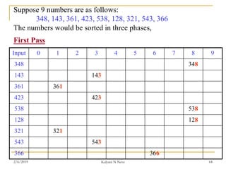
In radix sort, if numbers are present then,
In first pass, the numbers are sorted according to the units digits.
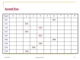
In second pass, the numbers are sorted according to the tens digit.
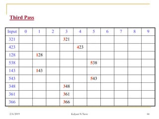
In third pass, the numbers are sorted according to the hundreds
digits. & so on.
2/6/2019 Kalyani N Neve 63
Suppose 9 numbers are as follows:
348, 143, 361, 423, 538, 128, 321, 543, 366
The numbers would be sorted in three phases,
First Pass
Input 0 1 2 3 4 5 6 7 8 9
348 348
143 143
361 361
423 423
538 538
128 128
321 321
543 543
366 366
2/6/2019 Kalyani N Neve 64
Second Pass
Input 0 1 2 3 4 5 6 7 8 9
361 361
321 321
143 143
423 423
543 543
366 366
348 348
538 538
128 128
2/6/2019 Kalyani N Neve 65
Third Pass
Input 0 1 2 3 4 5 6 7 8 9
321 321
423 423
128 128
538 538
143 143
543 543
348 348
361 361
366 366
2/6/2019 Kalyani N Neve 66
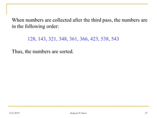
When numbers are collected after the third pass, the numbers are
in the following order:
128, 143, 321, 348, 361, 366, 423, 538, 543
Thus, the numbers are sorted.
2/6/2019 Kalyani N Neve 67
radix_sort(int arr[], int n)
{
int bucket[10][5],buck[10],b[10];
int i,j,k,l,num,div,large,passes;
div=1;
num=0;
large=arr[0];
for(i=0 ; i< n ; i++)
{
if(arr[i] > large)
{
large = arr[i];
}
while(large > 0)
{
num++;
large = large/10;
}
for(passes=0 ; passes < num ;
passes++)
{
for(k=0 ; k< 10 ; k++)
{
buck[k] = 0;
}
for(i=0 ; i< n ;i++)
{
l = ((arr[i]/div)%10);
bucket[l][buck[l]++] = arr[i];
}
i=0;
for(k=0 ; k < 10 ; k++)
{
for(j=0 ; j < buck[k] ; j++)
{
arr[i++] = bucket[k][j];
}
}
div*=10;
}}}
2/6/2019 Kalyani N Neve 68
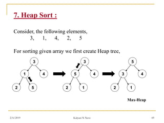
7. Heap Sort :
Consider, the following elements,
3, 1, 4, 2, 5
For sorting given array we first create Heap tree,
3
1 4
2 5
3
5 4
2 1
5
3 4
2 1
Max-Heap
2/6/2019 Kalyani N Neve 69
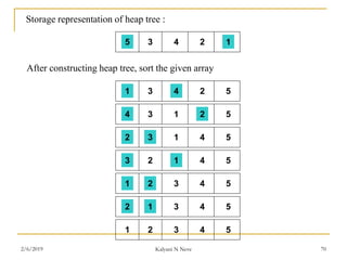
5 3 4 2 1
Storage representation of heap tree :
After constructing heap tree, sort the given array
1 3 4 2 5
4 3 1 2 5
2 3 1 4 5
3 2 1 4 5
1 2 3 4 5
2 1 3 4 5
1 2 3 4 5
2/6/2019 Kalyani N Neve 70
Searching:
Searching is used to find the location where an element is
available. There are two types of search techniques. They are:
1. Linear or sequential search
This is the simplest of all searching techniques.
In this technique, an ordered or unordered list will be
searched one by one from the beginning until the
desired element is found.
If the desired element is found in the list then the search
is successful otherwise unsuccessful.
2/6/2019 Kalyani N Neve 71
Suppose there are ‘n’ elements organized sequentially on a
List.
The number of comparisons required to retrieve an element
from the list, purely depends on where the element is stored in
the list.
If it is the first element, one comparison will do; if it is second
element two comparisons are necessary and so on.
On an average you need [(n+1)/2] comparison’s to search an
element.
If search is not successful, you would need ’n’ comparisons.
2/6/2019 Kalyani N Neve 72
Algorithm
Linear Search ( Array A, Value x)
Step 1: Set i to 1
Step 2: if i > n then go to step 7
Step 3: if A[i] = x then go to step 6
Step 4: Set i to i + 1
Step 5: Go to Step 2
Step 6: Print Element x Found at index i and go to step 8
Step 7: Print element not found
Step 8: Exit
2/6/2019 Kalyani N Neve 73
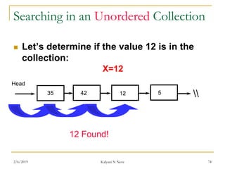
Searching in an Unordered Collection
 Let’s determine if the value 12 is in the
collection:
35 42 12 5 
12 Found!
Head
X=12
2/6/2019 Kalyani N Neve 74
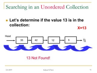
Searching in an Unordered Collection
 Let’s determine if the value 13 is in the
collection:
35 42 12 5 
13 Not Found!
Head
X=13
2/6/2019 Kalyani N Neve 75
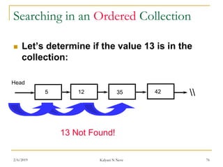
Searching in an Ordered Collection
 Let’s determine if the value 13 is in the
collection:
5 12 35 42 
13 Not Found!
Head
2/6/2019 Kalyani N Neve 76
2. BINARY SEARCH
If we have ‘n’ records which have been ordered by keys so that
x1 < x2 < … < xn .
When we are given a element ‘x’, binary search is used to find
the corresponding element from the list.
In case ‘x’ is present, we have to determine a value ‘j’ such that
a[j] = x(successful search).
If ‘x’ is not in the list then j is to set to zero (un successful
search).
2/6/2019 Kalyani N Neve 77
In Binary search we jump into the middle of the file, where we
find key a[mid], and compare ‘x’ with a[mid]. If x = a[mid] then
the desired record has been found.
If x < a[mid] then ‘x’ must be in that portion of the file that
precedes a[mid].
Similarly, if a[mid] > x, then further search is only necessary in
that part of the file which follows a[mid].
2/6/2019 Kalyani N Neve 78
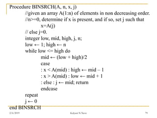
Procedure BINSRCH(A, n, x, j)
//given an array A(1:n) of elements in non decreasing order.
//n>=0, determine if x is present, and if so, set j such that
x=A(j)
// else j=0.
integer low, mid, high, j, n;
low ← 1; high ← n
while low <= high do
mid ← (low + high)/2
case
: x < A(mid) : high ← mid – 1
: x > A(mid) : low ← mid + 1
: else : j ← mid; return
endcase
repeat
j ← 0
end BINSRCH
2/6/2019 Kalyani N Neve 79
Binary search (Example)
 Example: Searching the array below for the value 42:
index 0 1 2 3 4 5 6 7 8 9 10 11 12 13 14 15 16
value -4 2 7 10 15 20 22 25 30 36 42 50 56 68 85 92 103
min mid max
Check A[mid]== number If yes PRINT
Check number<A[mid]
Check number>A[mid]
If yes min=mid+1
and repeat
If yes max=mid-1
and repeat
2/6/2019 Kalyani N Neve 80

Sorting and searching

  • 1.
  • 2.
    In computer science,a sorting algorithm is an algorithm that puts elements of a list in a certain order. Ordering the data in an increasing or decreasing fashion according to some relationship among the data item is called sorting. Efficient sorting is important for optimizing the use of other algorithms (such as search and merge algorithms) that require sorted lists to work correctly. Two main classification of sorting : 1. Internal Sorting Internal sorting is a process of sorting the data in the main memory. 2. External Sorting External sorting is process of sorting in which large blocks of data stored in storage devices are moved to the main memory and then sorted. 2/6/2019 Kalyani N Neve 2
  • 3.
    1.Insertion Sort : Supposean array A with n elements A[1], A[2],…..,A[n] is in memory. The insertion sort algorithm. Scans A from A[1] to A[n], inserting each element A[K] into its proper position in the previously sorted sub array A[1], A[2], …,A[K-1]. That is: Pass 1: A[1] by itself is trivially sorted. Pass 2: A[2] is inserted either before or after A[1] so that A[1], A[2] is sorted. Pass 3: A[3] is inserted into its proper place in A[1], A[2], that is before A[1], between A[1] and A[2], or after A[2], So that A[1], A[2],A[3] is sorted. 2/6/2019 Kalyani N Neve 3
  • 4.
    Pass 4: A[4]is inserted into its proper place in A[1],A[2],A[3] so that: A[1],A[2],A[3],A[4] is sorted. . . . . . Pass N : A[N] is inserted into its proper place in A[1],A[2],…,A[N-1] so that : A[1],A[2],……,A[N] is sorted. 2/6/2019 Kalyani N Neve 4
  • 5.
    Algorithm : INSERTION(A,N) 1. SetA[0] := -∞ [Initializes element] 2. Repeat Steps 3 to 5 for K = 2,3,…..,N: 3. Set TEMP := A[K] and PTR := K-1 4. Repeat while TEMP < A[PTR]: 1. Set A[PTR + 1] := A[PTR]. [Moves element forward.] 2. Set PTR := PTR – 1 5. Set A[PTR + 1] := TEMP [Inserts element in proper place.] [End of Step 2 loop.] 6. Return 2/6/2019 Kalyani N Neve 5
  • 6.
    Pass A[0] A[1]A[2] A[3] A[4] A[5] A[6] A[7] A[8] K=1: -∞ 33 44 11 88 22 66 55 K=2: -∞ 77 33 44 11 88 22 66 55 K=3: -∞ 33 77 44 11 88 22 66 55 K=4: -∞ 33 44 77 11 88 22 66 55 K=5: -∞ 11 33 44 77 88 22 66 55 K=6: -∞ 11 33 44 77 88 22 66 55 K=7: -∞ 11 22 33 44 77 88 66 55 K=8: -∞ 11 22 33 44 66 77 88 55 Sorted: -∞ 11 22 33 44 55 66 77 88 Array A is, 77, 33, 44, 11, 88, 22, 66, 55 77 2/6/2019 Kalyani N Neve 6
  • 7.
    2. Selection Sort: Suppose an array A with n elements A[1], A[2],…..,A[n] is in memory. The selection sort algo. For sorting A as follows: Pass 1: Find the location LOC of the smallest in the list of N elements A[1],A[2],….,A[N], and then interchange A[LOC] and A[1], Then : A[1] is sorted. Pass 2: Find the location LOC of the smallest in the sublist of N-1 elements A[1],A[2],….,A[N], and then interchange A[LOC] and A[2], Then : A[1], A[2]is sorted. Since A[1] <= A[2]. Pass 3:Find the location LOC of the smallest in the sub list of N-2 elements A[1],A[2],….,A[N], and then interchange A[LOC] and A[3], Then : A[1], A[2],A[3]is sorted. Since A[2] <= A[3]. 2/6/2019 Kalyani N Neve 7
  • 8.
    . . . Pass N-1:Find thelocation LOC of the smaller of the elements A[N-1],A[N], and then interchange A[LOC] and A[N- 1], Then : A[1],A[2],….A[N]is sorted. Since A[N-1] <= A[N]. Thus A is sorted after N-1 passes. 2/6/2019 Kalyani N Neve 8
  • 9.
    Algorithm : SELECTION(A,N) 1. RepeatSteps 2 and 3 for K=1,2,….,N-1 2. Call Min (A,K,N,LOC) 3. [Interchange A[K] and A[LOC]] Set TEMP := A[K], A[K] := A{LOC] and A[LOC] := TEMP [End of step 1 loop] 4. Exit MIN(A,K,N,LOC) 1. Set MIN := A[K] and LOC := K. [Initialize pointers] 2. Repeat for J=K+1,K+2,….,N If MIN > A[J], then : Set MIN := A[J] and LOC := A[J] and LOC := J [End of loop] 3. Return 2/6/2019 Kalyani N Neve 9
  • 10.
    Pass A[1] A[2]A[3] A[4] A[5] A[6] A[7] A[8] K=1: LOC=4 33 44 11 88 22 66 55 K=2: LOC=6 11 33 44 77 88 22 66 55 K=3: LOC=6 11 22 44 77 88 33 66 55 K=4: LOC=6 11 22 33 77 88 44 66 55 K=5: LOC=8 11 22 33 44 88 77 66 55 K=6: LOC=7 11 22 33 44 55 77 66 88 K=7: LOC=7 11 22 33 44 55 66 77 88 Sorted: 11 22 33 44 55 66 77 88 Array A is, 77, 33, 44, 11, 88, 22, 66, 55 77 2/6/2019 Kalyani N Neve 10
  • 11.
    3. Bubble Sort: Suppose an array A with n elements A[1], A[2],…..,A[n] is in memory. The bubble sort algo. For sorting A as follows: Step 1: Compare A[1] and A[2] and arrange them in the desired order, so that A[1] < A[2]. Then compare A[2] and A[3] and arrange them so that A[2] < A[3]. Continue until we compare A[N-1] with A[N] and arrange them. Step 2: Repeat step 1 with one less comparison, that is, now we stop after we compare and possibly rearrange A[N-1] and A[N-1]. . . . 2/6/2019 Kalyani N Neve 11
  • 12.
    Step N-1 :Compare A[1] with A[2] and arrange them so that A[1] < A[2]. After N-1 steps, the list will be sorted in increasing order. Suppose the following numbers are sorted in an array A : 32, 51, 27,85, 66, 23, 13, 57 We apply the bubble sort to the array A. 2/6/2019 Kalyani N Neve 12
  • 13.
    BUBBLE(DATA, N) Here DATAis an array with N elements. This algorithm sorts the elements in DATA. 1. Repeat steps 2 and 3 for K = 1 to N-1. 2. Set PTR := 1. [ Initialize pass pointer PTR] 3. Repeat while PTR <= N – K: [Execute pass] 1. If DATA[PTR] > DATA[PTR + 1], then : Interchange DATA[PTR] and DATA[PTR + 1] [End of If structure] 2. Set PTR := PTR + 1. [End of inner loop] [End of step 1 outer loop] 4. Exit 2/6/2019 Kalyani N Neve 13
  • 14.
    Pass 1: Wehave the following comparisons : 32 51 27 85 66 23 13 57 32 51 27 85 66 23 13 57 32 27 51 85 66 23 13 57 32 27 51 85 66 23 13 57 A1 A2< >A2 A3 <A3 A4 A4 A5> Not Altered Altered Not Altered Altered 2/6/2019 Kalyani N Neve 14
  • 15.
    32 27 5166 85 23 13 57 32 27 51 66 23 85 13 57 32 27 51 66 23 13 85 57 32 27 51 66 23 13 57 85 A5 A6> >A6 A7 >A7 A8 Altered Altered Altered At the end of first pass, the largest number, 85 has moved to the last position. 2/6/2019 Kalyani N Neve 15
  • 16.
    Pass 2 : 2733 51 66 23 13 57 85 27 33 51 23 66 13 57 85 27 33 51 23 13 66 57 85 27 33 51 23 13 57 66 85 A1 A2< A4 A5 A5 A6 A6 A7 Not Altered Altered Altered Altered 2/6/2019 Kalyani N Neve 16
  • 17.
    Pass 3 : 2733 23 51 13 57 66 85 27 33 23 13 51 57 66 85 27 23 33 13 51 57 66 85 27 23 13 33 51 57 66 85 A3 A4 A4 A5 A2 A3 A3 A4 Altered Altered Altered Altered Pass 4 : 2/6/2019 Kalyani N Neve 17
  • 18.
    23 27 1333 51 57 66 85 23 13 27 33 51 57 66 85 A1 A2 A2 A3 Altered Altered Pass 5 : 13 23 27 33 51 57 66 85 A1 A2 Altered Pass 6 : Pass 7 : Finally, A1 is compared with A2. No interchange takes place. Since the list is sorted. 2/6/2019 Kalyani N Neve 18
  • 19.
    4. Merge Sort: Suppose an array A with n elements A[1], A[2],…..,A[n] is in memory. The merge sort algorithm For sorting A as follows: 2/6/2019 Kalyani N Neve 19
  • 20.
    Kalyani N Neve Divideand Conquer  Recursive in structure  Divide the problem into sub-problems that are similar to the original but smaller in size  Conquer the sub-problems by solving them recursively. If they are small enough, just solve them in a straightforward manner.  Combine the solutions to create a solution to the original problem 2/6/2019 20
  • 21.
    Kalyani N Neve AnExample: Merge Sort Sorting Problem: Sort a sequence of n elements into non-decreasing order.  Divide: Divide the n-element sequence to be sorted into two subsequences of n/2 elements each  Conquer: Sort the two subsequences recursively using merge sort.  Combine: Merge the two sorted subsequences to produce the sorted answer. 2/6/2019 21
  • 22.
    Kalyani N Neve MergeSort – Example 18 26 32 6 43 15 9 1 18 26 32 6 43 15 9 1 18 26 32 6 43 15 9 1 2618 632 1543 19 18 26 32 6 43 15 9 1 18 26 32 6 43 15 9 1 18 26 326 15 43 1 9 6 18 26 32 1 9 15 43 1 6 9 15 18 26 32 43 18 26 18 26 18 26 32 32 6 6 32 6 18 26 32 6 43 43 15 15 43 15 9 9 1 1 9 1 43 15 9 1 18 26 32 6 43 15 9 1 18 26 632 626 3218 1543 19 1 915 43 16 9 1518 26 32 43 Original Sequence Sorted Sequence 2/6/2019 23
  • 23.
    MERGESORT(LOW, HIGH) 1. SetLOW := 1. 2. If LOW < HIGH: then: 1. Set MID := (LOW + N)/2 2. Call MERGESORT(LOW, MID) 3. Call MERGESORT(MID+1, HIGH) 4. Call MERGE(LOW,MID,HIGH) [End of step 2 loop] 7. Exit 2/6/2019 Kalyani N Neve 24
  • 24.
    MERGE(A, LOW, MID,HIGH) This algorithm merges two sorted sub arrays into one array. 1. [Initialize] h := LOW, i := LOW, j := MID + 1 2. Repeat while h <= MID && j <= HIGH: If A[h] <= A[j] then: Set b[i] := A[h] Set h := h +1 ELSE: Set b[i] := A[j] Set j := j +1 [End of If structure] Set i := i + 1 [End of loop] 2/6/2019 Kalyani N Neve 25
  • 25.
    3. If h> MID then: Set k := j Repeat while k <= HIGH Set h[i] := A[k] Set i := i + 1 ELSE Set k := h Repeat while k <= MID b[i] := a[k]; I := i+1; 4. Set k := LOW Repeat while k <= HIGH a[k] := b[k]; 5. Return 2/6/2019 Kalyani N Neve 26
  • 26.
    7 7 22 9 9 4 4 Low : 1 Mid : 2 High : 4 Low : 1 Mid : 1 High : 2 Low : 3 Mid : 3 High : 4 7, 2, 9, 4 2, 4, 7, 9 2, 77, 2 9, 4 4, 9 MergeSort(1,2) MergeSort(1,1) MergeSort(2,2) MergeSort(1,4) MergeSort(3,4) MergeSort(3,3) MergeSort(4,4) 2/6/2019 Kalyani N Neve 27
  • 27.
    5. Quick Sort: Quick sort is an algorithm of the divide-and-conquer type. Let us consider the following example with 13 elements to analyze quick sort: Select first element as the pivot element. Move ‘up’ pointer from left to right in search of an element larger than pivot. Move the ‘down’ pointer from right to left in search of an element smaller than pivot. If such elements are found, the elements are swapped. This process continues till the ‘up’ pointer crosses the ‘down’ pointer. If ‘up’ pointer crosses ‘down’ pointer, the position for pivot is found and interchange pivot and element at ‘down’ position. 2/6/2019 Kalyani N Neve 28
  • 28.
  • 29.
  • 30.
    Algorithm : Procedure QUICKSORT(p, q) integer p, q; global n, A(1:n) if p < q then j = q + 1 call PARTITION (p, j) call QUICKSORT (p, j – 1) // j is the position of partitioning element call QUICKSORT (j + 1, q) endif End QUICKSORT 2/6/2019 Kalyani N Neve 31
  • 31.
    Procedure PARTITION (m,p) integerm, p, i; global A(m:p) v ← A(m); i ← m //A(m) is the partition element loop loop i ← i + 1 until A(i) <= v repeat //i moves left to right loop p ← p – 1 until A(p) > v repeat //p moves right to left if i < p then call INTERCHANGE (A(i), A(p)) //exchange A(i) & A(p) else exit endif repeat A(m) ← A(p); A(p) ← v //partition element belongs at position p end PARTITION 2/6/2019 Kalyani N Neve 32
  • 32.
    Quicksort Algorithm Given anarray of n elements (e.g., integers):  If array only contains one element, return  Else  pick one element to use as pivot.  Partition elements into two sub-arrays:  Elements less than or equal to pivot  Elements greater than pivot  Quicksort two sub-arrays  Return results 2/6/2019 Kalyani N Neve 33
  • 33.
    Example We are givenarray of n integers to sort: 40 20 10 80 60 50 7 30 100 2/6/2019 Kalyani N Neve 34
  • 34.
    Pick Pivot Element Thereare a number of ways to pick the pivot element. In this example, we will use the first element in the array: 40 20 10 80 60 50 7 30 100 2/6/2019 Kalyani N Neve 35
  • 35.
    Partitioning Array Given apivot, partition the elements of the array such that the resulting array consists of: 1. One sub-array that contains elements >= pivot 2. Another sub-array that contains elements < pivot The sub-arrays are stored in the original data array. Partitioning loops through, swapping elements below/above pivot. 2/6/2019 Kalyani N Neve 36
  • 36.
    40 20 1080 60 50 7 30 100pivot_index = 0 [0] [1] [2] [3] [4] [5] [6] [7] [8] i j 2/6/2019 Kalyani N Neve 37
  • 37.
    40 20 1080 60 50 7 30 100pivot_index = 0 [0] [1] [2] [3] [4] [5] [6] [7] [8] i j 1. While data[i] <= data[pivot] ++i 2/6/2019 Kalyani N Neve 38
  • 38.
    40 20 1080 60 50 7 30 100pivot_index = 0 [0] [1] [2] [3] [4] [5] [6] [7] [8] i j 1. While data[i] <= data[pivot] ++i 2/6/2019 Kalyani N Neve 39
  • 39.
    40 20 1080 60 50 7 30 100pivot_index = 0 [0] [1] [2] [3] [4] [5] [6] [7] [8] i j 1. While data[i] <= data[pivot] ++i 2. While data[j] > data[pivot] --j 2/6/2019 Kalyani N Neve 40
  • 40.
    40 20 1080 60 50 7 30 100pivot_index = 0 [0] [1] [2] [3] [4] [5] [6] [7] [8] i j 1. While data[i] <= data[pivot] ++i 2. While data[j] > data[pivot] --j 2/6/2019 Kalyani N Neve 41
  • 41.
    40 20 1080 60 50 7 30 100pivot_index = 0 [0] [1] [2] [3] [4] [5] [6] [7] [8] i j 1. While data[i] <= data[pivot] ++i 2. While data[j] > data[pivot] --j 3. If i < j swap data[i] and data[j] 2/6/2019 Kalyani N Neve 42
  • 42.
    40 20 1030 60 50 7 80 100pivot_index = 0 i j 1. While data[i] <= data[pivot] ++i 2. While data[j] > data[pivot] --j 3. If i < j swap data[i] and data[j] [0] [1] [2] [3] [4] [5] [6] [7] [8] 2/6/2019 Kalyani N Neve 43
  • 43.
    40 20 1030 60 50 7 80 100pivot_index = 0 i j 1. While data[i] <= data[pivot] ++i 2. While data[j] > data[pivot] --j 3. If i < j swap data[i] and data[j] 4. While j > i, go to 1. [0] [1] [2] [3] [4] [5] [6] [7] [8] 2/6/2019 Kalyani N Neve 44
  • 44.
    40 20 1030 60 50 7 80 100pivot_index = 0 i j 1. While data[i] <= data[pivot] ++i 2. While data[j] > data[pivot] --j 3. If i < j swap data[i] and data[j] 4. While j > i, go to 1. [0] [1] [2] [3] [4] [5] [6] [7] [8] 2/6/2019 Kalyani N Neve 45
  • 45.
    40 20 1030 60 50 7 80 100pivot_index = 0 i j 1. While data[i] <= data[pivot] ++i 2. While data[j] > data[pivot] --j 3. If i < j swap data[i] and data[j] 4. While j > i, go to 1. [0] [1] [2] [3] [4] [5] [6] [7] [8] 2/6/2019 Kalyani N Neve 46
  • 46.
    40 20 1030 60 50 7 80 100pivot_index = 0 i j 1. While data[i] <= data[pivot] ++i 2. While data[j] > data[pivot] --j 3. If i < j swap data[i] and data[j] 4. While j > i, go to 1. [0] [1] [2] [3] [4] [5] [6] [7] [8] 2/6/2019 Kalyani N Neve 47
  • 47.
    40 20 1030 60 50 7 80 100pivot_index = 0 i j 1. While data[i] <= data[pivot] ++i 2. While data[j] > data[pivot] --j 3. If i < j swap data[i] and data[j] 4. While j > i, go to 1. [0] [1] [2] [3] [4] [5] [6] [7] [8] 2/6/2019 Kalyani N Neve 48
  • 48.
    40 20 1030 60 50 7 80 100pivot_index = 0 i j 1. While data[i] <= data[pivot] ++i 2. While data[j] > data[pivot] --j 3. If i < j swap data[i] and data[j] 4. While j > i, go to 1. [0] [1] [2] [3] [4] [5] [6] [7] [8] 2/6/2019 Kalyani N Neve 49
  • 49.
    1. While data[i]<= data[pivot] ++i 2. While data[j] > data[pivot] --j 3. If i < j swap data[i] and data[j] 4. While j > i, go to 1. 40 20 10 30 7 50 60 80 100pivot_index = 0 i j [0] [1] [2] [3] [4] [5] [6] [7] [8] 2/6/2019 Kalyani N Neve 50
  • 50.
    1. While data[i]<= data[pivot] ++i 2. While data[j] > data[pivot] --j 3. If i < j swap data[i] and data[j] 4. While j > i, go to 1. 40 20 10 30 7 50 60 80 100pivot_index = 0 i j [0] [1] [2] [3] [4] [5] [6] [7] [8] 2/6/2019 Kalyani N Neve 51
  • 51.
    1. While data[i]<= data[pivot] ++i 2. While data[j] > data[pivot] --j 3. If i < j swap data[i] and data[j] 4. While j > i, go to 1. 40 20 10 30 7 50 60 80 100pivot_index = 0 i j [0] [1] [2] [3] [4] [5] [6] [7] [8] 2/6/2019 Kalyani N Neve 52
  • 52.
    1. While data[i]<= data[pivot] ++i 2. While data[j] > data[pivot] --j 3. If i < j swap data[i] and data[j] 4. While j > i, go to 1. 40 20 10 30 7 50 60 80 100pivot_index = 0 i j [0] [1] [2] [3] [4] [5] [6] [7] [8] 2/6/2019 Kalyani N Neve 53
  • 53.
    1. While data[i]<= data[pivot] ++i 2. While data[j] > data[pivot] --j 3. If i < j swap data[i] and data[j] 4. While j > i, go to 1. 40 20 10 30 7 50 60 80 100pivot_index = 0 i j [0] [1] [2] [3] [4] [5] [6] [7] [8] 2/6/2019 Kalyani N Neve 54
  • 54.
    1. While data[i]<= data[pivot] ++i 2. While data[j] > data[pivot] --j 3. If i < j swap data[i] and data[j] 4. While j > i, go to 1. 40 20 10 30 7 50 60 80 100pivot_index = 0 i j [0] [1] [2] [3] [4] [5] [6] [7] [8] 2/6/2019 Kalyani N Neve 55
  • 55.
    1. While data[i]<= data[pivot] ++i 2. While data[j] > data[pivot] --j 3. If i < j swap data[i] and data[j] 4. While j > i, go to 1. 40 20 10 30 7 50 60 80 100pivot_index = 0 i j [0] [1] [2] [3] [4] [5] [6] [7] [8] 2/6/2019 Kalyani N Neve 56
  • 56.
    1. While data[i]<= data[pivot] ++i 2. While data[j] > data[pivot] --j 3. If i < j swap data[i] and data[j] 4. While j > i, go to 1. 40 20 10 30 7 50 60 80 100pivot_index = 0 i j [0] [1] [2] [3] [4] [5] [6] [7] [8] 2/6/2019 Kalyani N Neve 57
  • 57.
    1. While data[i]<= data[pivot] ++i 2. While data[j] > data[pivot] --j 3. If i < j swap data[i] and data[j] 4. While j > i, go to 1. 40 20 10 30 7 50 60 80 100pivot_index = 0 i j [0] [1] [2] [3] [4] [5] [6] [7] [8] 2/6/2019 Kalyani N Neve 58
  • 58.
    1. While data[i]<= data[pivot] ++i 2. While data[j] > data[pivot] --j 3. If i < j swap data[i] and data[j] 4. While j > i, go to 1. 5. Swap data[j] and data[pivot_index] 40 20 10 30 7 50 60 80 100pivot_index = 0 i j [0] [1] [2] [3] [4] [5] [6] [7] [8] 2/6/2019 Kalyani N Neve 59
  • 59.
    1. While data[i]<= data[pivot] ++i 2. While data[j] > data[pivot] --j 3. If i < j swap data[i] and data[j] 4. While j > i, go to 1. 5. Swap data[j] and data[pivot_index] 7 20 10 30 40 50 60 80 100pivot_index = 4 i j [0] [1] [2] [3] [4] [5] [6] [7] [8] 2/6/2019 Kalyani N Neve 60
  • 60.
    Partition Result 7 2010 30 40 50 60 80 100 <= data[pivot] > data[pivot] [0] [1] [2] [3] [4] [5] [6] [7] [8] 2/6/2019 Kalyani N Neve 61
  • 61.
    Recursion: Quicksort Sub-arrays 720 10 30 40 50 60 80 100 <= data[pivot] > data[pivot] [0] [1] [2] [3] [4] [5] [6] [7] [8] 2/6/2019 Kalyani N Neve 62
  • 62.
    6. Radix Sort: Radix sort is a method can be used to sort a list of names alphabetically. To sort alphabetically radix is 26, the 26 letters of the alphabet. In radix sort, if numbers are present then, In first pass, the numbers are sorted according to the units digits. In second pass, the numbers are sorted according to the tens digit. In third pass, the numbers are sorted according to the hundreds digits. & so on. 2/6/2019 Kalyani N Neve 63
  • 63.
    Suppose 9 numbersare as follows: 348, 143, 361, 423, 538, 128, 321, 543, 366 The numbers would be sorted in three phases, First Pass Input 0 1 2 3 4 5 6 7 8 9 348 348 143 143 361 361 423 423 538 538 128 128 321 321 543 543 366 366 2/6/2019 Kalyani N Neve 64
  • 64.
    Second Pass Input 01 2 3 4 5 6 7 8 9 361 361 321 321 143 143 423 423 543 543 366 366 348 348 538 538 128 128 2/6/2019 Kalyani N Neve 65
  • 65.
    Third Pass Input 01 2 3 4 5 6 7 8 9 321 321 423 423 128 128 538 538 143 143 543 543 348 348 361 361 366 366 2/6/2019 Kalyani N Neve 66
  • 66.
    When numbers arecollected after the third pass, the numbers are in the following order: 128, 143, 321, 348, 361, 366, 423, 538, 543 Thus, the numbers are sorted. 2/6/2019 Kalyani N Neve 67
  • 67.
    radix_sort(int arr[], intn) { int bucket[10][5],buck[10],b[10]; int i,j,k,l,num,div,large,passes; div=1; num=0; large=arr[0]; for(i=0 ; i< n ; i++) { if(arr[i] > large) { large = arr[i]; } while(large > 0) { num++; large = large/10; } for(passes=0 ; passes < num ; passes++) { for(k=0 ; k< 10 ; k++) { buck[k] = 0; } for(i=0 ; i< n ;i++) { l = ((arr[i]/div)%10); bucket[l][buck[l]++] = arr[i]; } i=0; for(k=0 ; k < 10 ; k++) { for(j=0 ; j < buck[k] ; j++) { arr[i++] = bucket[k][j]; } } div*=10; }}} 2/6/2019 Kalyani N Neve 68
  • 68.
    7. Heap Sort: Consider, the following elements, 3, 1, 4, 2, 5 For sorting given array we first create Heap tree, 3 1 4 2 5 3 5 4 2 1 5 3 4 2 1 Max-Heap 2/6/2019 Kalyani N Neve 69
  • 69.
    5 3 42 1 Storage representation of heap tree : After constructing heap tree, sort the given array 1 3 4 2 5 4 3 1 2 5 2 3 1 4 5 3 2 1 4 5 1 2 3 4 5 2 1 3 4 5 1 2 3 4 5 2/6/2019 Kalyani N Neve 70
  • 70.
    Searching: Searching is usedto find the location where an element is available. There are two types of search techniques. They are: 1. Linear or sequential search This is the simplest of all searching techniques. In this technique, an ordered or unordered list will be searched one by one from the beginning until the desired element is found. If the desired element is found in the list then the search is successful otherwise unsuccessful. 2/6/2019 Kalyani N Neve 71
  • 71.
    Suppose there are‘n’ elements organized sequentially on a List. The number of comparisons required to retrieve an element from the list, purely depends on where the element is stored in the list. If it is the first element, one comparison will do; if it is second element two comparisons are necessary and so on. On an average you need [(n+1)/2] comparison’s to search an element. If search is not successful, you would need ’n’ comparisons. 2/6/2019 Kalyani N Neve 72
  • 72.
    Algorithm Linear Search (Array A, Value x) Step 1: Set i to 1 Step 2: if i > n then go to step 7 Step 3: if A[i] = x then go to step 6 Step 4: Set i to i + 1 Step 5: Go to Step 2 Step 6: Print Element x Found at index i and go to step 8 Step 7: Print element not found Step 8: Exit 2/6/2019 Kalyani N Neve 73
  • 73.
    Searching in anUnordered Collection  Let’s determine if the value 12 is in the collection: 35 42 12 5 12 Found! Head X=12 2/6/2019 Kalyani N Neve 74
  • 74.
    Searching in anUnordered Collection  Let’s determine if the value 13 is in the collection: 35 42 12 5 13 Not Found! Head X=13 2/6/2019 Kalyani N Neve 75
  • 75.
    Searching in anOrdered Collection  Let’s determine if the value 13 is in the collection: 5 12 35 42 13 Not Found! Head 2/6/2019 Kalyani N Neve 76
  • 76.
    2. BINARY SEARCH Ifwe have ‘n’ records which have been ordered by keys so that x1 < x2 < … < xn . When we are given a element ‘x’, binary search is used to find the corresponding element from the list. In case ‘x’ is present, we have to determine a value ‘j’ such that a[j] = x(successful search). If ‘x’ is not in the list then j is to set to zero (un successful search). 2/6/2019 Kalyani N Neve 77
  • 77.
    In Binary searchwe jump into the middle of the file, where we find key a[mid], and compare ‘x’ with a[mid]. If x = a[mid] then the desired record has been found. If x < a[mid] then ‘x’ must be in that portion of the file that precedes a[mid]. Similarly, if a[mid] > x, then further search is only necessary in that part of the file which follows a[mid]. 2/6/2019 Kalyani N Neve 78
  • 78.
    Procedure BINSRCH(A, n,x, j) //given an array A(1:n) of elements in non decreasing order. //n>=0, determine if x is present, and if so, set j such that x=A(j) // else j=0. integer low, mid, high, j, n; low ← 1; high ← n while low <= high do mid ← (low + high)/2 case : x < A(mid) : high ← mid – 1 : x > A(mid) : low ← mid + 1 : else : j ← mid; return endcase repeat j ← 0 end BINSRCH 2/6/2019 Kalyani N Neve 79
  • 79.
    Binary search (Example) Example: Searching the array below for the value 42: index 0 1 2 3 4 5 6 7 8 9 10 11 12 13 14 15 16 value -4 2 7 10 15 20 22 25 30 36 42 50 56 68 85 92 103 min mid max Check A[mid]== number If yes PRINT Check number<A[mid] Check number>A[mid] If yes min=mid+1 and repeat If yes max=mid-1 and repeat 2/6/2019 Kalyani N Neve 80