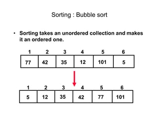
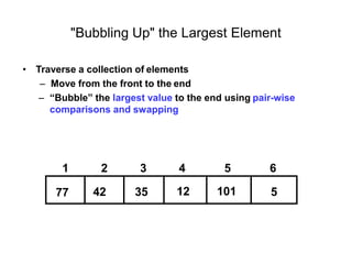
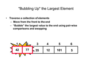
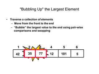
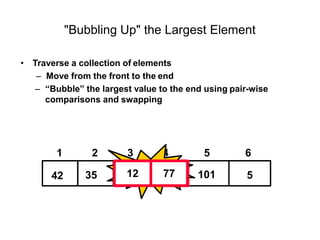
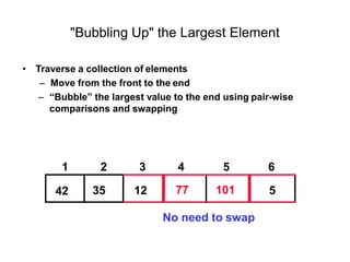
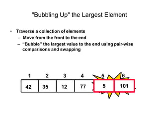
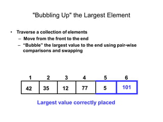
The document discusses the array data structure and the bubble sort algorithm. Key points: - An array is a linear data structure that stores elements in contiguous memory locations. It is defined by its size and elements can be accessed via indices. - Bubble sort works by repeatedly "bubbling up" the largest value to its sorted position. It compares adjacent elements and swaps them if out of order. 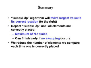- The bubble sort algorithm takes O(n^2) time since in the worst case, each of the n passes could involve n-1 swaps. It is one of the simplest sorting algorithms but has poor time complexity.

1. CSE225: Data Structures and Algorithms
Lecture 3:Array

2. Array
Data structures are classified as either linear or nonlinear.
A data structure is said to be linear if its elements form a sequence or a linear
list.
There are two basic ways of representing such linear structures in memory.
One way is to have the linear relationship between the elements represented
by means of sequential memory locations. These linear structures are called
arrays.
The other way is to have the linear relationship between the elements
represented by means of pointers or links. These linear structures are called
linked lists.
Nonlinear structures are trees and graphs.

3. Linear Arrays
A linear array is a list of finite number n of homogeneous data elements such that :
a) The elements of the array are referenced respectively by an index set
consisting of n consecutive numbers.
b) The elements of the array are stored respectively in successive memory
locations.
The number n of elements is called the length or size of the array.
Three numbers define an array : lower bound, upper bound, size.
a. The lower bound is the smallest subscript you can use in the array (usually 0)
b. The upper bound is the largest subscript you can use in the array
c. The size / length of the array refers to the number of elements in the array , It
can be computed as upper bound - lower bound + 1
Let, Array name is A then the elements of A is : a1,a2….. an
Or by the bracket notation A[1], A[2], A[3],…………., A[n]
The number k in A[k] is called a subscript and A[k] is called a subscripted variable.

4. Linear Arrays
Example :
A six element linear array DATAconsisting of the integers.
247
56
429
135
87
156
DATA[1] = 247
DATA[2] = 56
DATA[3] = 429
DATA[4] = 135
DATA[5] = 87
DATA[6] = 156
1
2
3
4
5
6
DATA

5. Linear Arrays
Example :
An automobile company uses an array AUTO to record the number of auto mobile
sold each year from 1932 through 1984.
AUTO[k] = Number of auto mobiles sold in the year K
LB = 1932
UB = 1984
Length = UB – LB+1 = 1984 – 1930+1 =55

6. Representation of linear array in memory
Let LA be a linear array in the memory of the computer. The memory of the
computer is a sequence of addressed locations.
LA
1000
1001
1002
1003
1004
1005
Fig : Computer memory
The computer does not need to keep track of the
address of every element of LA, but needs to keep
track only of the first element of LA, denoted by
Base(LA)
Called the base address of LA. Using this address
Base(LA), the computer calculates the address of
any element of LA by the following formula :
LOC(LA[k]) = Base(LA) + w(K – lower bound)
Where w is the number of words per memory cell for
the array LA

7. Representation of linear array in memory
Example :
An automobile company uses an array AUTO to record
the number of auto mobile sold each year from 1932
through 1984. Suppose AUTO appears in memory as
pictured in fig A . That is Base(AUTO) = 200, and w =4
words per memory cell for AUTO. Then,
LOC(AUTO[1932]) = 200, LOC(AUTO[1933]) =204
LOC(AUTO[1934]) = 208
the address of the array element for the year K = 1965
can be obtained by using :
LOC(AUTO[1965]) = Base(AUTO) + w(1965 – lower
bound)
=200+4(1965-1932)=332
200
201
202
203
204
205
206
207
208
209
210
211
212
Fig :A
AUTO[1932]
AUTO[1933]
AUTO[1934]

8. Traversing linear arrays
Print the contents of each element of DATA or Count the number of elements
of DATA with a given property. This can be accomplished by traversing DATA,
That is, by accessing and processing (visiting) each element of DATA exactly
once.
Algorithm 2.3: Given DATAis a linear array with lower bound LB and
upper bound UB . This algorithm traverses DATAapplying an operation
PROCESS to each element of DATA.
1. Set K : = LB.
2. Repeat steps 3 and 4 while K<=UB:
3. Apply PROCESS to DATA[k]
4. Set K : = K+1.
5. Exit.

9. Example :
An automobile company uses an array AUTO to record the number of auto
mobile sold each year from 1932 through 1984.
a)Find the number NUM of years during which more than 300 automobiles
were sold.
b) Print each year and the number of automobiles sold in that year
Traversing linear arrays
1. Set NUM : = 0.
2. Repeat for K = 1932 to 1984:
if AUTO[K]> 300, then : set NUM : = NUM+1
3. Exit.
1.Repeat for K = 1932 to 1984:
Write : K,AUTO[K]
2. Exit.

10. Inserting and Deleting
Inserting refers to the operation of adding another element to the Array
Deleting refers to the operation of removing one element from the Array
Inserting an element somewhere in the middle of the array require that each
subsequent element be moved downward to new locations to accommodate the
new element and keep the order of the other elements.
Deleting an element somewhere in the middle of the array require that each
subsequent element be moved one location upward in order to “fill up” the
array. Fig shows Milon Inserted, Sumona deleted.
Dalia Rahaman
Sumona
Mubtasim Fuad
Anamul Haque
1
2
3
4
5
6
STUDENT
Dalia Rahaman
Sumona
Milon
Mubtasim Fuad
Anamul Haque
1
2
3
4
5
6
STUDENT
Dalia Rahaman
Milon
Mubtasim Fuad
Anamul Haque
1
2
3
4
5
6
STUDENT

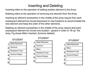
11. INSERTING AN ELEMENT INTO AN ARRAY:
Insert (LA, N, K, ITEM)
Here LA is linear array with N elements and K is a positive integer such that
K<=N.This algorithm inserts an element ITEM into the Kth position in LA.
ALGORITHM
Step 1.
Step 2.
Step 3.
Step 4.
[Initialize counter] Set J:=N
Repeat Steps 3 and 4] while J>=K
[Move Jth element downward] Set LA [J+1]: =LA[J]
[Decrease counter] Set J:=J-1
[End of step 2 loop]
Step 5
Step 6.
Step 7.
[Insert element] Set LA [K]: =ITEM
[Reset N] Set N:=N+1
Exit
Insertion

12. DELETING AN ELEMENT FROM A LINEAR ARRAY
Delete (LA, N, K, ITEM)
ALGORITHM
Step 1.
Step 2.
Set ITEM: = LA[K]
Repeat for J=K to N-1
[Move J+1st element upward] Set LA [J]: =LA[J+1]
[End of loop]
Step 3
Step 4.
[Reset the number N of elements in LA] Set N:=N-1
Exit
Deletion

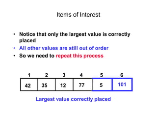
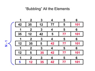
14. Bubble sort
Bubble sort is one of the easiest sort algorithms. It is called bubble sort because
it will 'bubble' values in your list to the top.
Algorithm Bubble_Sort (DATA, N):
1. Repeat steps 2 and 3 for K = 1 to N-1.
2. Set PTR: =1.[Initializes pass pointer PTR]
3. Repeat while PTR<=N-K: [Executes pass]
a) If DATA[PTR]>DATA[PTR+1],then:
TEMP := A[PTR], A[PTR] := A[PTR+1], A[PTR+1] := temp
[End of if structure]
b) Set PTR: =PTR+1
[End of inner loop]
[End of step 1 Outer loop]
4. Exit

15. • Sorting takes an unordered collection and makes
it an ordered one.
1 2 3 4 5 6
77 42 35 12 101 5
1 2 3 4 5 6
5 12 35 42 77 101
Sorting : Bubble sort

16. "Bubbling Up" the Largest Element
• Traverse a collection of elements
– Move from the front to the end
– “Bubble” the largest value to the end using pair-wise
comparisons and swapping
77 42 35 12 101 5
1 2 3 4 5 6

17. "Bubbling Up" the Largest Element
• Traverse a collection of elements
– Move from the front to the end
– “Bubble” the largest value to the end using pair-wise
comparisons and swapping
5
12
35 101
1 2 3 4 5 6
77Swap
42
42 77

18. "Bubbling Up" the Largest Element
• Traverse a collection of elements
– Move from the front to the end
– “Bubble” the largest value to the end using pair-wise
comparisons and swapping
5
12
42 101
1 2 3 4 5 6
77 Swap
35
35 77

19. "Bubbling Up" the Largest Element
• Traverse a collection of elements
– Move from the front to the end
– “Bubble” the largest value to the end using pair-wise
comparisons and swapping
5
35
42 101
1 2 3 4 5 6
77Swap
12
12 77

20. "Bubbling Up" the Largest Element
• Traverse a collection of elements
– Move from the front to the end
– “Bubble” the largest value to the end using pair-wise
comparisons and swapping
42 35 12 77 101 5
1 2 3 4 5 6
No need to swap

21. "Bubbling Up" the Largest Element
• Traverse a collection of elements
– Move from the front to the end
– “Bubble” the largest value to the end using pair-wise
comparisons and swapping
77
12
35
42
1 2 3 4 5 6
101S
w
ap 5
5 101

22. "Bubbling Up" the Largest Element
• Traverse a collection of elements
– Move from the front to the end
– “Bubble” the largest value to the end using pair-wise
comparisons and swapping
42 35 12 77 5 101
1 2 3 4 5 6
Largest value correctly placed

23. Putting It All Together

24. Items of Interest
• Notice that only the largest value is correctly
placed
• All other values are still out of order
• So we need to repeat this process
42 35 12 77 5 101
1 2 3 4 5 6
Largest value correctly placed

25. Repeat “Bubble Up” How Many Times?
• If we have N elements…
• And if each time we bubble an element, we
place it in its correct location…
• Then we repeat the “bubble up” process N – 1
times.
• This guarantees we’ll correctly
place all N elements.

26. “Bubbling” All the Elements
1 2 3 4 5 6
42 35 12 77 5 101
1 2 3 4 5 6
35 12 42 5 77 101
1 2 3 4 5 6
12 35 5 42 77 101
1 2 3 4 5 6
12 5 35 42 77 101
1 2 3 4 5 6
5 12 35 42 77 101
N
-
1

27. Summary
• “Bubble Up” algorithm will move largest value to
its correct location (to the right)
• Repeat “Bubble Up” until all elements are
correctly placed:
– Maximum of N-1 times
– Can finish early if no swapping occurs
• We reduce the number of elements we compare
each time one is correctly placed

28. Complexity of the bubble sort algorithm
The time for a sorting algorithm is measured in terms of the number of
comparisons. The number f(n) of comparisons in the bubble sort is easily
computed. Specifically there are n -1 comparisons during first pass, which places
the largest element in the last position, there are n -2 comparisons in the second
step, which places the second largest element in the next – to - last position, and
so on. Thus
f(n) = (n-1)+(n-2)+. . . +2+1 =n(n-1)/2=n2/2+O(n)
In other words, The time required to execute bubble sort algorithm is proportional
to n2, where n is the number of input items.