This master's thesis addresses the problem of loop closure detection in visual SLAM. Two approaches using binary features are presented: 1) A probabilistic approach called FAB-MAP is adjusted to use binary features for reliable loop closure detection. 2) A novel approach measures similarity between VLAD representations of image frames combined with pre-filtering to improve detection rate and speed. Both approaches are implemented and evaluated in the ORB-SLAM2 framework on the KITTI dataset, showing they achieve similar trajectory accuracy as ORB-SLAM2 while saving considerable time in loop detection compared to the original method.


![Chapter 1
Introduction
1.1 Motivation
For several decades, the autonomous mobile robots have been developed and applied in
various areas of daily life, like scientific research, industry production and personal service.
Modern robotic applications require robots not only to respond to human’s instructions but
also to observe and understand the world. With the advent of cheap and well-performing
camera sensors, it is easy and realistic to integrate a visual system in robots. As a result,
applications based on visual information become the priority of development.
In particular, autonomous navigation, which is the concern of my thesis, increasingly de-
pends on visual information. The robots must have the ability to identify its location and
create a map of its environment. In order to satisfy these requirements, some robots make
use of external infrastructure such as the Global Positioning System (GPS), which makes
the navigation process very efficient [CN08]. But in many cases, as the external infrastruc-
ture is unreachable in some environment like indoor, underwater or outer space, robots
must navigate based on their internal sensors. In this situation, autonomous navigation
based on visual information becomes a reliable and efficient solution. This kind of navi-
gation problem without any external assistant is referred to as Simultaneous Localization
and Mapping (SLAM).
Simultaneous Localization and Mapping (SLAM)
SLAM is a general concept rather than an algorithm, which becomes a core field of re-
search in today’s robotic applications development. SLAM consists of many different com-
ponents, each component realizes a specific function and supported by many different
algorithms, Figure 1.1 shows a simple example of SLAM structure. Basic theories are the
support of SLAM system, like Extended Kalman Filter (EKF) [SSC90] and Particle Filter](https://image.slidesharecdn.com/c23b7113-893c-4f39-bb28-73befa7b3431-161213205645/85/Master_Thesis_Jiaqi_Liu-6-320.jpg)
![CHAPTER 1. INTRODUCTION 2
(PF) [MTK+
02] were the popular approximate methods for traditional solutions. SLAM
problem can be classified into different directions based on the choice of input sensor, and
in this thesis we focus on the solutions for the problem with camera as input sensor, which
is called visual SLAM. In the modern visual SLAM concept, three main tasks should be
accomplished simultaneously. The first one is local mapping and there are different kinds
of maps generated as a result, the choice of map depends strongly on the basic theory.
Second one is local tracking which realizes functions like initial pose estimation, global
relocalization, local map tracking and so on, each function can be implemented by differ-
ent algorithms. The last one is loop closure, which is the main concern in this thesis and
introduced in the following section.
Fab-Map
SLAM
Mapping
Sensor Advanced Topic
Basic Theory
Camera Laser Sonar
Sparse(Semi-) Dense
Relocal-
ization
Pose
Estimation
Dynamic Coordinate Sensor Fusion
Bayesian Optimization
PF
EKF
G2O
Bag of Words
Tracking Loop Closure
Figure 1.1: Example of SLAM structure. The Loop Closure block is the concern of this
thesis.](https://image.slidesharecdn.com/c23b7113-893c-4f39-bb28-73befa7b3431-161213205645/85/Master_Thesis_Jiaqi_Liu-7-320.jpg)
![CHAPTER 1. INTRODUCTION 3
Loop Closure Detection
In order to accomplish real world tasks, robots must be able to recognize re-visited loca-
tions which already exist in the map, and at the same time correct the accumulated error
of previous processes to avoid a noticeable drift in the map. To solve these problems,
a research field called loop closure detection was introduced, which is also an important
component of SLAM. Loop closure detection problem can be interpreted as a place recog-
nition problem. To solve this problem, the simplest way is to compare the similarity of
images. There are several approaches for that, among them one typical way is to compare
descriptors of feature points. However, it is not suitable for modern applications because of
high computation complexity. Thus a compact image representation was proposed which
is called Bag of Words (BoW) [SZ03, BMM07] representation. It is efficient for image
matching, but because of perceptual aliasing and perceptual repetition it does not pro-
vide a reliable performance. In order to increase the degree of precision, an algorithm
called FAB-MAP [CN08] was proposed. It was proven to work well both for small-scale
and large-scale environment. However, its efficiency can’t satisfy nowadays real-time tasks
gradually. Therefore, a high-efficient and reliable loop closure detection method is needed.
Our approaches in this thesis allow robots to identify current location as previous visited
locations correctly and speed-up the loop detection process as much as possible.
1.2 Problem Formulation and Challenges
The problem which we aim to solve in this thesis can be described as following: Are
the observations derived from two different sequences or images collected from the same
location [Cum09] and if so, can the robot realize this fact fast enough to accomplish a
real-time task?
To solve this problem, we may encounter several difficulties like following in the real world:
1. The environment is always changing. Although the robot stays in the same location,
the observations still vary due to changes of weather, season, lighting, viewpoint or
movement of objects, etc. This kind of fact results in huge variation of appearance
information, especially brings difficulties for feature points extraction and match-
ing. Figure 1.2 shows two images which were taken at the same location, but because
of the objects’ movement, 40% less feature points were detected in the right image. If
we define the state that images are matched as positive, then this situation produces
more false negatives.](https://image.slidesharecdn.com/c23b7113-893c-4f39-bb28-73befa7b3431-161213205645/85/Master_Thesis_Jiaqi_Liu-8-320.jpg)
![CHAPTER 1. INTRODUCTION 4
Figure 1.2: Different observations from the same location at different time points. The
feature points are extracted by FAST detector.
2. The objects in the environment are visually repetitive [Cum09]. In contrast to the
first problem, sometimes we may get similar observations in different locations. Fig-
ure 1.3 shows two images from two locations with distance 100m. Although the
locations are different, similar appearance information is extracted. It is hard for
robots to distinguish different locations based on these kind of observations, which
contributes to more false positives.
Figure 1.3: Observations from two different locations with distance 100m. The feature
points are extracted by FAST detector.
3. For large-scale scenarios, as the number of locations in the map increasing, it is time-
consuming to compare the similarity of image pairs. And for real-time SLAM, several
threads are required to run in parallel and each thread has its specific functions. In
this case, time control becomes the prior task in this kind of system. Usually loop
closure detection and loop correction are treated as one thread as in [MAMT15], so
if loop detection consumes too much time, it would slow down and sometimes even
break down the whole system.
4. In most modern systems, in order to perform place recognition or image matching,
feature point descriptions or compact image representations should be stored in the
local memory. However, for large-scale scenarios which contain more than 1000 im-
ages, the systems would suffer from the lack of memory. In this case, loop closure
detection is limited by the allocation of memory. Thus a method based on low di-
mensional image representations is needed.](https://image.slidesharecdn.com/c23b7113-893c-4f39-bb28-73befa7b3431-161213205645/85/Master_Thesis_Jiaqi_Liu-9-320.jpg)
![CHAPTER 1. INTRODUCTION 5
1.3 Contributions and Outline
In order to overcome above difficulties, our approaches in this thesis make following con-
tributions:
1. To the best of our knowledge, it is the first time to combine the well-known FAB-
MAP algorithm with binary features to perform reliable loop closure detection. For
many robotic applications, binary features are more suitable to be extracted than
traditional floating point features (SURF, SIFT, etc.), and it is also efficient for image
matching. Our experimental results from evaluation in ORB-SLAM2 framework on
KITTI dataset [GLU12] prove that FAB-MAP performs also well in a SLAM system
based on binary features.
2. Three novel algorithms by using VLAD [JDSP10] representation with binary features
instead of BoW are proposed to achieve faster loop closure detection rate.
(a) Comparing similarity between VLAD signatures of image pairs without any
pre-filter mechanism.
(b) Increasing the loop closure detection rate by using hierarchical multi-VLAD
signatures to pre-filter the most likely loop candidates and verify the true one.
(c) Further accelerate loop closure detection process by applying a product quan-
tization scheme combined with inverted index search to realize early unlikely-
candidates rejection and extract the true loop candidates.
All three algorithms above have been implemented in ORB-SLAM2 framework and
evaluated on the KITTI dataset, the experimental results show that all loops are
detected and the average detection time reduces significantly compared to the build-
in algorithm of ORB-SLAM2.
The remainder of this thesis is structured as follows. In Chapter 2, we discuss about
the related work in robot navigation and the development of solutions for visual SLAM.
Moreover, we also introduce the basic principle of ORB-SLAM2 framework in detail, which
is used for evaluation of our approaches. Chapter 3 describes a probabilistic model called
FAB-MAP and introduces the implementation in ORB-SLAM2 to detect loops by using
binary features. In addition, the experimental results from evaluation performed on KITTI
dataset are presented and discussed. Chapter 4 presents a novel approach to accomplish
loop closure detection by using VLAD representations. And three different algorithms for
this approach are introduced separately. The evaluation results for all three algorithms are
shown at the end of this chapter. Conclusions are presented in Chapter 5.](https://image.slidesharecdn.com/c23b7113-893c-4f39-bb28-73befa7b3431-161213205645/85/Master_Thesis_Jiaqi_Liu-10-320.jpg)
![Chapter 2
Related Work
2.1 SLAM Overview
Simultaneous localization and mapping (SLAM) is the problem of describing the surround-
ing world and generating the map based on observations perceived by sensors in real time,
while simultaneously locating itself in the environment. SLAM involves a moving agent
(for example a robot), which is equipped at least one sensor (a camera, a laser, a sonar)
and able to gather information about its surroundings. One goal of a SLAM system is
to generate a probability distribution of the robot’s location and estimate the spatial re-
lationship between observations from different locations. Depending on the choice how
to represent the observations and how to estimate the locations’ probability distribution,
there are various SLAM approaches. In this section, we first introduce two prominent
SLAM concepts generally, then introduce more specific the development of visual SLAM
systems with camera as sensor.
2.1.1 Solutions to the SLAM Problem: Filters in SLAM
Extended Kalman Filter SLAM
The first approach is Extended Kalman Filter SLAM (EKF-SLAM) which was introduced
by Smith, Self and Cheeseman [SSC90] in 1990. In this work, the authors define a spatial
representation which is called the stochastic map, where the objects at these locations
are represented by a set of landmarks. The map contains the spatial relationship among
objects, which also includes the landmarks’ uncertainties and covariances. These param-
eters are approximated by Gaussian distributions. Although the EKF-SLAM provides
a significant improvement and are widely used, it still suffers from the issues like high
computational complexity, linearization and the Gaussian well-approximation assumption.](https://image.slidesharecdn.com/c23b7113-893c-4f39-bb28-73befa7b3431-161213205645/85/Master_Thesis_Jiaqi_Liu-11-320.jpg)
![CHAPTER 2. RELATED WORK 7
For the computational complexity, the sensor updating time has a quadratic relationship
with the number of landmarks h. For h landmarks which are preserved by the Kalman
filters, the covariance matrix has h2
size, and if only one single landmark is updated, the
whole covariance matrix has to be recomputed. So the complexity O(h2
) limits the usage
of EKF-SLAM for large-scale environment with more than hundred landmarks.
Another issue is the incorrect usage of Kalman filter for non-linear process. Kalman filter
[Kal60] is designed for only linear processes. However, in order to apply Kalman filter,
EKF-SLAM linearizes all estimation functions which are non-linear. This approximation
will result in huge errors in practice if the function lies far away of linear. To make an
improvement, the Iterated Extended Kalman Filter (IEKF) [BSLK04] and the Unscented
Kalman Filter (UKF) [JU97] were proposed. But still linearization error can’t be avoided
within the EKF framework.
Finally, the assumption that all the means and covariances of landmarks can be well
approximated by Gaussian distributions is not the real case in the world. Treating the
dynamical world environment as a single distribution would lead to wrong estimations of
the map. To deal with this, another concept called Particle Filter SLAM was proposed.
Particle Filter SLAM
In order to apply SLAM in large-scale environment, Montemerlo, Thrun, Koller and Weg-
breit in 2002 introduced an efficient SLAM algorithm based on Rao-Blackwellized particle
filter, called FastSLAM [MTK+
02] and later improved in [MSDB03]. FastSLAM simplifies
the SLAM as a problem of identifying the robot’s location and the estimation of landmarks.
This algorithm estimates the posterior probability over robot trajectory by using particle
filters, where each particle possesses h EKFs to estimate h landmark positions. Compare
to EKF-SLAM, this algorithm does not have the linearization issue and the complexity
reduces to O(ph), where p is the number of particles and h is the number of landmarks.
Additionally, the authors also developed a tree-based data structure, which further re-
duces the complexity to O(p log h). Based on that, FastSLAM is much faster than the
EKF-SLAM, which makes it optimal for applications in large-scale environment. More-
over, this algorithm can also be used for situations with unknown number of landmarks,
this property enables it to provide solutions for all the SLAM problems.
This algorithm indeed reduces the complexity for estimation significantly, however, to
generate the particle filters itself is time-consuming. Additionally, particle filters are non-
deterministic. Particles will become non-diversity over long trajectory, because at a re-
sampling step during filter updates, one state already occupied more particles will gain
even more particles than other states. Over time, the particles will converge to one state.
So this algorithm only suits system that does not preserve its history trajectory, which
means the current state is independent from previous ones. This property results in that
FastSLAM can’t create a high-quality consistency map of long trajectory with loops.](https://image.slidesharecdn.com/c23b7113-893c-4f39-bb28-73befa7b3431-161213205645/85/Master_Thesis_Jiaqi_Liu-12-320.jpg)
![CHAPTER 2. RELATED WORK 8
2.1.2 Visual SLAM
Based on the choice of the input sensor, SLAM can be classified into laser-based, sonar-
based and camera-based systems. With the advent of high-quality and low-cost camera
sensors, it is intuitive to integrate visual systems in robots, which provide visual information
to help robots understand the world. So several approaches to solve the SLAM problem by
using appearance information has been developed in the recent past, often referred visual
SLAM. Here the so-called appearance information refers to the feature point descriptions
or the pixel intensity values of images. Based on these two different representations of
appearance information, the approaches of SLAM can be classified into two sets. One set
of approaches create a dense or semi-dense map for SLAM by directly using pixel intensity
values and minimizing the photometric error, called direct SLAM. This set of approaches
can describe the environment more concretely. However, this kind of approaches have
higher computation complexity, which are not suitable for real-time SLAM.
The most representative dense approach was proposed by Newcombe et al., called DTAM
[NLD11]. DTAM is a system which relies on every pixel methods and accelerated by
GPU hardware for real-time performance. However, it is not invariant to the change of
illumination and easily affected by dynamic elements. Later, a semi-dense approach LSD-
SLAM was proposed by Engel et al. [ESC14]. In addition to dense tracking and mapping
by using pixel intensity values directly, it also extracts feature points from key-frames to
detect loops by using FAB-MAP algorithm.
The other set of approaches use descriptors of feature points extracted from key-frames
as appearance information, which are called featured-based approaches. Although these
approaches can only describe the surrounding environment with sparse representations,
SLAM system can benefit from their efficiency and invariance towards change of viewpoints,
scale and intensity values. So the featured-based approach is more suited for real-time
applications, which is also the concern of this thesis.
The most representative featured-based approach is PTAM [KM07], which was the first
work to propose the idea of splitting tracking and mapping into two separate tasks, running
in parallel threads. This innovation makes the real-time SLAM system come true. However,
PTAM can’t detect large loops because the map points are only used for tracking but not
for place recognition.
Strasdat et al. [SMD10] proposed a large-scale monocular SLAM system by using a new
image processing method front-end combined with a sliding-window Bundle Adjustment
(BA) [TMHF99], which can track hundreds of features per frame. For loop closure detec-
tion, it uses SURF features as appearance information to find the loop candidates, then
followed by a 7DoF pose graph optimization to correct the loop. Subsequently, a double
window optimization framework was proposed in 2011 by Strasdat et al. [SDMK11]. It
performs BA in the inner window and pose graph optimization in the outer window of a
limited-size. The point-pose constraints in an outer window support the constraints in an](https://image.slidesharecdn.com/c23b7113-893c-4f39-bb28-73befa7b3431-161213205645/85/Master_Thesis_Jiaqi_Liu-13-320.jpg)
![CHAPTER 2. RELATED WORK 9
inner window. And the pose constraints are based on covisibility graph, which is also used
in ORB-SLAM [MAMT15].
Another relative complete system, which includes loop closing, relocalization and the work
to deal with dynamic environment, was proposed by Pirker et al. [PRB11], called CD-
SLAM. This system is also a feature-based SLAM and it defines a specific rule to select
key-frames, which prevents from an unbounded increasing map size. To handle the long-
term dynamics of environment, it uses the Histogram of Oriented Cameras (HoC) descriptor
[PRB10] to represent a map point. However, the authors of this system haven’t published
a public implementation, so it is difficult to make a comparison.
Based on the main theory of PTAM, another approach was proposed in 2015 by Mur-
Artal et al., which is called ORB-SLAM [MAMT15]. This approach uses ORB to detect
and describe feature points as visual cues, and combines the place recognition technology
in [GLT12] and the work of Strasdat et al. [SMD10] to detect loops. ORB-SLAM cre-
ates three threads to run in parallel: tracking, local mapping and loop closure detection.
Moreover, this algorithm is extended to create a semi-dense map [MAT15], which provides
more information about the environment. The details of ORB-SLAM are introduced in
section 2.4.
2.2 Place Recognition
2.2.1 Feature Point Detectors
As mentioned previously, visual SLAM is an appearance-based concept, which means we
need to collect enough useful appearance information from the observations at the begin-
ning of the whole process. Usually the appearance information refers to feature points in
images or videos. To accomplish this goal, a reliable, robust and effective detection method
is needed.
In the past half century, a large number of feature points detectors have been proposed.
Among them, SIFT [Low99] and SURF [BETVG08] have been testified as the suitable
detectors and implemented in many different robotic applications. Although these two
detection methods can offer good performance, they are unable to meet the growing real-
time requirements gradually. So some other time-effective algorithms are developed for use
in real-time or low-power applications on a mobile robot, which have limited computational
resources. The most typical one is FAST corner detector [RD05]. FAST is an efficient
method to find feature points in real-time systems, but for performance, unlike SURF and
SIFT, FAST doesn’t include an orientation operator. For this reason, it has been adjusted
to Oriented-FAST [RRKB11] by using the centroid technique derived from the reference
paper by Rosin [Ros99] to offer better performance, which can satisfy the requirements of
nowadays applications.](https://image.slidesharecdn.com/c23b7113-893c-4f39-bb28-73befa7b3431-161213205645/85/Master_Thesis_Jiaqi_Liu-14-320.jpg)
![CHAPTER 2. RELATED WORK 10
2.2.2 Feature Point Descriptors
Image local feature descriptors are descriptions derived from the feature contents of im-
ages and videos, which describe elementary characteristics of objects in frames such as
shape, color, texture or motion. As a result, visual descriptors are produced by feature
points detectors. With the development of detection methods, a wide variety of image
local feature descriptors have also been proposed. Similar to SIFT detector, the SIFT
descriptor [Low99] also plays a very important role in the field of computer vision. Based
on the concept of SIFT descriptor, SURF descriptor [BETVG08] was proposed to acceler-
ate computation process. However, both SIFT and SURF descriptors are stored by using
floating point numbers, for SIFT 128 dimensional vector, it takes 512 bytes to store one
descriptor. Similarly, a 64 dimensional SURF vector also requires 256 bytes. This kind
of vectors representing thousands features needs a lot of memory, which also increases
the matching time and the computation time of the following process in visual SLAM. So
binary descriptor becomes the first choice for most real-time systems.
As a typical binary feature descriptor, BRIEF (Binary Robust Independent Elementary
Features) [CLSF10] was introduced in 2010 as an alternative of SIFT and SURF descriptors.
BRIEF uses small smooth image patches, in each patch it selects a set of location pairs
with prior fixed pattern, and compares the intensity value for each pair, then produces the
result 1 or 0. For matching, Hamming Distance is used to match these descriptors. This
realizes a fast matching speed because the Hamming distance is the sum of the bitwise XOR
operation, which is more efficient than the Euclidean distance computation. So BRIEF is
a faster method for feature description computing and matching in comparison with SIFT
and SURF descriptors. However, BRIEF is sensitive to in-plane rotation. Thus it has
been adjusted as Rotation-Aware BRIEF [RRKB11], which uses less-correlated intensity
comparisons to provide better performance.
2.2.3 Detector and Descriptor used in this Thesis
As discussed above, the traditional SIFT and SURF are not optimal for nowadays robotic
applications. Considering the computation cost, matching performance and memory
limitation, fast detection method and binary description of feature points become the
prior technology for real-time systems. So ORB (Oriented FAST and Rotated BRIEF)
[RRKB11] was introduced in 2011, which combines FAST feature detector and BRIEF
descriptor with modifications to achieve good performance.
oFAST (Oriented FAST)
FAST is an efficient method to find key-points, and after filtering by Harris corner mea-
surement, several top quality points among the original key-points are extracted, still it](https://image.slidesharecdn.com/c23b7113-893c-4f39-bb28-73befa7b3431-161213205645/85/Master_Thesis_Jiaqi_Liu-15-320.jpg)
![CHAPTER 2. RELATED WORK 11
must use pyramid schemes for scale to produce multiscale-features [KM08]. Moreover, it
was modified to oFAST by authors to compute the orientation.
oFAST defines image patch around corner with radius r, and in this patch it computes
an intensity centroid [Ros99] and the direction of vector from corner to centroid produces
the orientation. And to compute the centroid, two gradient-based measures BIN and
MAX are used. For both case, horizontal and vertical gradients are calculated first, then
MAX chooses the largest gradient in the corner patch. Similar to SIFT, BIN generates a
10-degree-interval histogram of gradient directions and among them the maximum bin is
chosen [RRKB11].
rBRIEF (Rotated BRIEF)
BRIEF is a binary local feature descriptor, which has an efficient performance in terms
of computation and matching. However, it is very sensible to in-plane rotation, with a
rotation of a few degrees, the matching performance falls off sharply. To solve this problem,
a steered BRIEF according to the orientation of key-points has been proposed [RRKB11].
For a location (xi,yi), assuming s binary tests are made, then a 2×s matrix M are defined,
which stores the coordinates of these tested pixels. The corresponding rotation matrix Rθ
derived from the orientation of patch θ with M produces the steered version Mθ. The
authors also discretize the angle into 12 degrees, and a lookup table is constructed to pre-
compute BRIEF patterns. Then ORB applies a greedy search among all binary tests to
find the most uncorrelated ones, which have high variance and whose mean values are close
to 0.5, to get the rBRIEF result.
In the paper [RRKB11], the authors have made several experiments to verify that ORB
outperforms SIFT and SURF in both matching performance and computation time. For
example, Table 2.1 is collected from the experiment by running a single thread code on an
Intel i7 2.8GHz processor, which shows that ORB is 13 times faster than SURF, and more
than 300 times faster than SIFT. Therefore, based on the superiority of ORB and inspired
by the work of ORB-SLAM [MAMT15], we decide to use ORB to detect and describe
feature points, which offers visual cues for our approaches.
Table 2.1: Average computation time over 24 640 × 480 images from the Pascal dataset
[RRKB11,EVGW+
10]
Detector ORB SURF SIFT
Time per frame (ms) 15.3 217.3 5228.7](https://image.slidesharecdn.com/c23b7113-893c-4f39-bb28-73befa7b3431-161213205645/85/Master_Thesis_Jiaqi_Liu-16-320.jpg)
![CHAPTER 2. RELATED WORK 12
2.2.4 Compact Image Representation
For place recognition, matching feature descriptors of observations from different loca-
tions is the simplest way. However, it becomes computationally difficult for real-time task
with large-scale scenarios. So the concept of compact image representation has been pro-
posed in recent years considering the efficiency of matching and less memory consuming.
Nowadays, two compact image representations are well used, one is BoW (Bag of Words)
representation and the other is VLAD (Vector of Locally Aggregated Descriptors) repre-
sentation [JDSP10].
Bag of Words (BoW)
BoW is computed from local descriptors, so it preserves the most part of visual information.
Moreover, it is a single high dimensional vector for one image, which can be compared with
standard distances.
The BoW model groups all local descriptors as a training dataset, and a visual vocabulary
of size k is learned based on this dataset by using clustering algorithms. Each visual word
in the vocabulary is a local descriptor, which represents the centroid of one cluster. All
descriptors are compared with the centroids by using standard distances to find the nearest
neighbor of each descriptor, then are labelled by cluster indices. The BoW representation
is a k bins histogram, which shows the frequencies of visual words (clusters) existing in
one image. The whole process is illustrated by Figure 2.1.
Bag of Words has a very effective and reliable image matching performance, so it is usually
directly used for loop detection by measuring similarity in visual SLAM. However, due to
the problems of perceptual aliasing and perceptual repetition, it is always not the best
choice. In another perspective, because of its efficiency and accuracy, it is usually con-
sidered as the basis of advanced loop closure algorithms, such as FAB-MAP [CN08] and
DBoW2 [GLT12].
Until now, the most BoW representations are calculated from floating point local descrip-
tors like SURF or SIFT. As one main motivation of this thesis, we want to use binary
features for generating BoW representations, and based on them verify if FAB-MAP algo-
rithm still performs well with binary features.
Vector of Locally Aggregated Descriptor (VLAD)
Although BoW provides higher efficiency in terms of matching compared to local descrip-
tors, it still has limitations. The performance of BoW depends on the size of vocabulary,
from observation of experiments, the bigger the vocabulary size is, the better the perfor-
mance is, until a certain saturation, where the clustering is too fine grained. However,](https://image.slidesharecdn.com/c23b7113-893c-4f39-bb28-73befa7b3431-161213205645/85/Master_Thesis_Jiaqi_Liu-17-320.jpg)
![CHAPTER 2. RELATED WORK 13
(a) Extract features
(b) Learn visual vocabulary
(c) Represent images by frequencies of visual words
Figure 2.1: Bag of Words for image clustering [Li11].
bigger vocabulary size brings two problems: high computation cost and more memory con-
sumption. So a more effective representation was proposed in 2010, which is called Vector
of Locally Aggregated Descriptors (VLAD) [JDSP10].
Similar to BoW, VLAD is also a single high dimensional vector which describes one image.
In addition, VLAD includes the difference information between descriptors and cluster
centroids, which provides higher accuracy. VLAD requires far less dimensions than BoW
to obtain the same performance [JDSP10], which reduces memory consumption and also
computation time significantly. So VLAD representation is more suitable for large-scale
environment than BoW.
The VLAD model also needs to train a visual vocabulary, and the training process is
similar to BoW model. After arranging all descriptors to the vocabulary, the differences
between descriptor and centroid in each cluster are computed. At last, all differences in
each cluster are accumulated as one vector, these vectors are then normalized to generate
VLAD signature. The general idea is illustrated by Figure 2.2 and described in Chapter 4
in more detail.
Because of high accuracy and fast matching speed, it is effective to detect loops by simply
measuring similarity between VLAD signatures with pre-filter technique. Based on that,
another main goal of this thesis is to evaluate the performance of VLAD representation for
loop closure detection in visual SLAM.](https://image.slidesharecdn.com/c23b7113-893c-4f39-bb28-73befa7b3431-161213205645/85/Master_Thesis_Jiaqi_Liu-18-320.jpg)
![CHAPTER 2. RELATED WORK 14
(a) Learn visual vocabulary and cluster descriptors
(b) Compute differences
(c) Accumulate differences in each cluster
Figure 2.2: VLAD signature generation. Here, c represents the cluster centroid, x is a new
local descriptor and v is one residual vector which is one component of the final VLAD
signature [Li15].
2.3 Recent Work for Loop Closure Detection
To solve the loop closing problem in visual SLAM, a place recognition system should
be used, which recognizes the previous map area. In this section, we talk about the
development of loop closing algorithms by using different place recognition systems in the
recent work.
In 2011, Williams et al. [WKR11] proposed a relocalization module based on the work
[LF06], which is used for loop closing and relocalization in a filter-based monocular SLAM.
This module makes binary tests randomly for image patches and classifies them with binary
score lists to find the correspondences between local image features and map features. The
score lists are trained off-line from thousands of patches which are generated by warping or
obtained from live videos. However, it requires 1.25Mb memory to store one map feature](https://image.slidesharecdn.com/c23b7113-893c-4f39-bb28-73befa7b3431-161213205645/85/Master_Thesis_Jiaqi_Liu-19-320.jpg)
![CHAPTER 2. RELATED WORK 15
class, which may suffer from the lack of memory for a large-scale environment [MAT14].
Eade et al. [ED08] proposed a work, which unifies loop closing and relocalization in a graph
SLAM system based on the BoW appearance model. Unlike the typical training process for
visual vocabulary, the authors build it incrementally during operation based on 16-SIFT
descriptors. Strasdat et al. [SDMK11] and Lim et al. [LFP11] use tree-structured BoW
appearance model to identify loop candidates with covisibility graph. The hierarchical vo-
cabulary tree is trained from SURF descriptors. In 2012, G´alvez-L´opez et al. proposed the
work DBoW2 [GLT12] to detect loops by using a binary tree-structured BoW appearance
model. DBoW2 trains the visual vocabulary off-line from a large set of binary descrip-
tors like BRIEF or ORB. Each BoW vector contains the term frequency-inverse document
frequency (tf-idf) score, and use the L1-score as the similarity measurement for one BoW
vector pair.
In 2008, Cummins et al. [CN08] proposed a fast appearance-based place recognition algo-
rithm based on BoW representation, which is called FAB-MAP. They generate a location
distribution based on the correlation information between visual words in one BoW vector.
The visual vocabulary is trained from SURF descriptors. Pirker et al. [PRB11] integrate
the FAB-MAP algorithm in a monocular SLAM thought for dynamic world, called CD
SLAM. As a result, the loop closing process realized by FAB-MAP with pose optimization
requires 5ms on average.
2.4 ORB-SLAM System
ORB-SLAM is a relative complete SLAM system which uses ORB to detect and describe
feature points. It uses this kind of features to offer appearance information for all tasks.
Because of fast computing and matching speed, ORB features make the whole system
more efficient and more suitable for real-time applications. To satisfy real-time require-
ments, ORB-SLAM has three threads running in parallel: tracking, local mapping and
loop closing.
To generate the map, ORB-SLAM uses key-frames to represent camera locations with
matched map points. Based on the relationship of each key-frame, the covisibility graph,
the spanning tree and the essential graph are defined. For loop closure detection, a place
recognition module is integrated in the system, which is provided by DBoW2 [GLT12]. All
components in ORB-SLAM are shown in Figure 2.3.
2.4.1 Map and Place Recognition Module
Similar to PTAM [KM07], ORB-SLAM defines a policy (section 2.4.2) to select key-frames
instead of all frames to reduce computational cost, which makes bundle adjustment (BA)
[TMHF99] more suitable for real-time SLAM. Each key-frame is generated in tracking](https://image.slidesharecdn.com/c23b7113-893c-4f39-bb28-73befa7b3431-161213205645/85/Master_Thesis_Jiaqi_Liu-20-320.jpg)
![CHAPTER 2. RELATED WORK 16
Extract
ORB
Initial Pose Estima-
tion from last frame
or Relocation
Track Local
Map
New Key-frame
Decision
Pose
Optimization
Frame
Key-frame
Key-frame
Inseration
Recent Map-
Points Culling
New Map
Points Creation
Local BA
Local Key-
frames Culling
Optimize
Essential
Graph
Loop
Fusion
Compute
Sim3
Candidates
Dtection
Loop Closing
Tracking
Local Mapping
MAP
MapPoints
Key-frame
Covisibilty
Graph
Essential
Graph
Spanning
Tree
Visual
Vocabulary
Recognition
Database
Place Recongition
Figure 2.3: ORB-SLAM system overview, showing the tracking, local mapping and loop
closing threads. The place recognition module and the map are also illustrated. Adapted
from [MAMT15].
thread and should contain the camera pose, the camera intrinsics, ORB features and the
selected compact image representation. Moreover, for long-life operation, some redundant
key-frames are discarded as time goes by.
Each map point, which is successfully tracked based on the key-frames, contains the 3D
position, the viewing direction, the corresponding ORB descriptor and the invariance region
in which it can be observed. In the local mapping thread, some untracked map points are
culled based on a strict mechanism (section 2.4.3).
Based on the relationships of key-frames, the covisibility graph, the spanning tree and the
essential graph were proposed in ORB-SLAM. Covisibility graph is an undirected weighted
graph [SDMK11] with each key-frame as a node. If two key-frames share observations of](https://image.slidesharecdn.com/c23b7113-893c-4f39-bb28-73befa7b3431-161213205645/85/Master_Thesis_Jiaqi_Liu-21-320.jpg)
![CHAPTER 2. RELATED WORK 17
at least 15 common map points, an edge between these two key-frames are created and
weighted by the number of common points. Spanning tree is a subgraph of covisibility graph
with the same number of nodes and minimal edges. Essential graph is also a subgraph of
covisibility graph, which includes the spanning tree, the edges with relative larger weight
and also the loop closure edges. It generates a strong network of cameras, and distributes
the loop closing errors along the network. This property helps the pose graph optimization
[SMD10] for loop correction to get effective and accurate results.
To identify the loop candidates, a place recognition module is integrated in the system,
which contains a general visual vocabulary and a recognition database. The visual vo-
cabulary is trained off-line with ORB descriptors obtained from a large dataset. To make
searching more efficient, the system builds an invert index database for every visual word of
the vocabulary. In this database, corresponds to the index of a visual word, all key-frames
are stored in which this visual word can be observed. When a key-frame is inserted or
culled, the system updates database instantaneously.
2.4.2 Tracking Thread
The first task of tracking thread is to extract ORB features of the current frame. Then an
estimation for initial pose of camera is made. However, for the camera pose estimation,
two cases should be considered, one is if tracking was not successful for last frame, the
estimation should be made via global relocalization [MAMT15] by using the PnP algorithm
[LMNF09]. For the other case, if tracking was successful, a constant velocity motion model
is used to predict initial pose of camera. For both cases, the camera pose of current frame
is optimized.
After initial camera pose estimation, two sets of frames are defined, one is a set of all
previous key-frames which share map points with the current frame, and the other is a
group with all neighbor frames in covisibility graph of the first set. All map points which
are seen in these two sets are filtered by following criteria [MAMT15]:
1. The projection of the map point in the current frame should not beyond the image
bounds.
2. The angle between the current viewing direction v and the mean viewing ray r of the
map point should fulfil the relationship v · r ≥ cos(60◦
).
3. The distance between the map point and camera center should be limited within the
scale invariance region.
Based on the map points in the current frame, the camera pose is optimized.
Another function of tracking thread is to decide if the current frame is a new key-frame.
Unlike PTAM [KM07], ORB-SLAM defines five conditions [MAMT15] to test the current
frame. The conditions are defined as following:](https://image.slidesharecdn.com/c23b7113-893c-4f39-bb28-73befa7b3431-161213205645/85/Master_Thesis_Jiaqi_Liu-22-320.jpg)

![CHAPTER 2. RELATED WORK 19
are two requirements should be fulfilled. First, the map point should be found in at least
25% of the frames in which it is expected to be observed. Second, the map point must
be observed in at least three key-frames, if there are more than one key-frame has passed
from the map point creation. This test can guarantee the map points are retained in the
map, and prevents from the wrong triangulation.
Another function of local mapping thread is to create new map points. These points are
created by triangulating ORB features from connected key-frames in the covisibility graph.
If ORB features in current frame are not matched, then matches are searched with other
unmatched points in other key-frames. In addition, this thread also discards matches which
do not meet the epipolar equation.
One important task of local mapping thread is to apply the local bundle adjustment. This
adjustment optimizes the current key-frame, its neighbors in covisibility graph and all the
map points from these key-frames, which provides accurate estimations of camera locations.
In order to keep the efficiency of the whole system, this thread also realizes a function
to filter out the redundant key-frames. Inspired by the work [TLD+
13], it deletes all the
neighbor key-frames of current frame in covisibility graph, whose 90% map points have
been observed in other three or more key-frames within the same or finer scale [MAMT15].
The process of local mapping thread is shown in Figure 2.5.
Key-frame exists in the queue ?
Map Points Culling
Create New Map Points
Local Bundle Adjustment
Insert Key-frame
Local Key-frames Culling
Yes
No
Figure 2.5: Local Mapping Thread in ORB-SLAM2.](https://image.slidesharecdn.com/c23b7113-893c-4f39-bb28-73befa7b3431-161213205645/85/Master_Thesis_Jiaqi_Liu-24-320.jpg)
![CHAPTER 2. RELATED WORK 20
2.4.4 Loop Closing Thread
The main goal of loop closing thread is to treat the last key-frame as the observation of
the current location, and apply an algorithm to detect and close loops.
For loop candidates detection, ORB-SLAM computes the similarity of BoW representations
between current key-frame and its all neighbors in the covisibility graph, and defines the
L1-score of image pairs as the similarity score, in between a maximal score Smax is found.
This operation is realized by a binary Bag of Words implementation DBoW2 [GLT12]. If
any previous key-frame, which does not connect to the current key-frame, obtain a score
larger than Smax, then it is treated as a loop candidate. However, there may be several loop
candidates for the current frame because of similar BoW representations, so the similarity
transformation computation is needed, which can check if the loop candidate is true.
The similarity transformation computation serves as geometrical validation of the loop. At
first, 3D to 3D correspondences are found by using correspondences of ORB descriptors
between the current frame and one loop candidate. Then ORB-SLAM uses the method
of Horn [Hor87] to compute a similarity sim, and if sim has enough inliers, the loop with
this loop candidate is identified as a true one.
Based on sim and the correction of camera pose corresponding to the current key-frame,
loop can be fused and new edges in the covisibility graph are inserted. This step serves as
the first step of loop correction. Moreover, in order to correct the scale drift [SMD10] and
close the loop efficiently, a pose graph optimization over the essential graph is performed.
Functions of loop closing thread are presented in Figure 2.6.
Key-frame exists in the queue ?
Loop Candidates Detection
Compute Similarity Transformation
Loop Correction
Yes
Yes
Yes
No
No
No
Figure 2.6: Loop Closing Thread in ORB-SLAM2.](https://image.slidesharecdn.com/c23b7113-893c-4f39-bb28-73befa7b3431-161213205645/85/Master_Thesis_Jiaqi_Liu-25-320.jpg)
![Chapter 3
FAB-MAP Model with Binary
Features
This chapter introduces a probabilistic model for loop closure detection using appearance
information, which is called Fast Appearance Based Mapping (FAB-MAP) [CN08]. The
basic theory of this model is to compute a probability distribution over camera locations
and to decide whether the current observations derived from a new place or the previous
existing places in the map. This approach is inspired by the Bag of Words (BoW) im-
age retrieval system, but unlike the previous solutions by simply measuring appearance
similarity, FAB-MAP uses a generative model to find the dependence relationship between
visual words and use this information to compute the probability that the new observations
obtained from old places.
FAB-MAP has been proved that it performs well for on-line loop closure in real-time tasks.
However, as the application of ORB in nowadays SLAM systems becomes popular, it has
not been tested if it still can provide good performance with binary features. So the focus
in this chapter will be on the validation of the binary FAB-MAP. For evaluation purpose,
we implement FAB-MAP in the ORB-SLAM2 framework to replace original loop closure
detection algorithm, and the experiment details are introduced in section 3.4.
3.1 Appearance Representation and Location Repre-
sentation
FAB-MAP treats the world as a set of discrete locations and each location is described
by appearance observations like image or video. Incoming appearance information is con-
verted into a BoW representation, more specific each visual word represents the presence
or absence of one cluster in the current observation instead of representing frequencies. As-
suming we have trained a vocabulary with size k. A BoW representation of an observation](https://image.slidesharecdn.com/c23b7113-893c-4f39-bb28-73befa7b3431-161213205645/85/Master_Thesis_Jiaqi_Liu-26-320.jpg)
![CHAPTER 3. FAB-MAP MODEL WITH BINARY FEATURES 22
captured at time t is denoted as Zt = {z1, ..., zk}, where zi is a binary variable indicating
the presence or absence of the i-th word of the vocabulary. Furthermore, Zt
is defined for
representing a set of all BoW representations originated from observations up to time t.
Similar to the appearance representation, Lt
= {L1, ..., Lnt } represents the map at time t,
which is a set of nt discrete and disjoint locations. So the appearance model of a location
is the probability about the existence of visual word zi:
Lq : {p(z1 = 1|Lq), ..., p(zk = 1|Lq)}. (3.1)
This simple appearance and location model serve as the basis of FAB-MAP algorithm.
3.2 Approximating Discrete Probability Distribu-
tions with Dependence Trees
From the previous section, the probability that the specific observation is collected at
one location can be defined as a distribution P(Z). This distribution is generated on k
discrete variables Z = {z1, z2, ..., zk}, whose parameters need to be learned from previous
observations. However, this kind of k-th order discrete probability distribution will become
intractable when k increases significantly. So Lewis [Lew59] and Brown [Bro59] proposed a
solution to approximate a k-th order distribution by a product of its lower order component
distributions. Still it is very difficult to find a method for choosing the best set of component
distributions to obtain a proper approximation. In 1968, Chow and Liu [CL68] provided
a solution to approximate a k-th order distribution by a product of k − 1 second-order
component distributions with dependence trees, which is called Chow-Liu-Tree.
3.2.1 Chow-Liu-Tree
For a k-th order discrete probability distribution, there are k(k − 1)/2 second-order dis-
tributions. If we treat every variable as a node in an undirected graph G, then there are
k(k − 1)/2 edges connecting each node, shown in Figure 3.1 left. Among them, at most
k − 1 component distributions can be used for distribution approximation, in other words,
only k − 1 edges are preserved to generate the dependence tree, shown in Figure 3.1 right.
Then the distribution is approximated as following:
P(Z) =
k
i=1
p(Zmi
|Zmj(i)
), 0 ≤ j(i) < i, (3.2)
where (m1, ..., mk) is an unknown permutation of integers 1, 2, ..., k, and each variable can
be conditioned upon at most one other variable.](https://image.slidesharecdn.com/c23b7113-893c-4f39-bb28-73befa7b3431-161213205645/85/Master_Thesis_Jiaqi_Liu-27-320.jpg)
![CHAPTER 3. FAB-MAP MODEL WITH BINARY FEATURES 23
Z1
Z2
Z3 Z4
Z5
Z1
Z2
Z3 Z4
Z5
Z1
Z2
Z3 Z4
Z5
Figure 3.1: Left: Graph of the underlying distribution P(Z). The edges are weighted by
mutual information between variables. The edges that contribute to the maximal sum of
branch weights are shown by the solid lines. Middle: Naive Bayes approximation. Right:
Chow-Liu-Tree [CN08].
In order to measure the goodness of approximation, a notion for closeness of approximation
has been defined. At first, we assume P(Z) and Pa(Z) be two probability distributions on
k discrete variables Z = {z1, z2, ..., zk}. The Kullback-Leibler divergence I(P(Z), Pa(Z))
[KL51] is defined as following:
I(P(Z), Pa(Z)) =
Z
P(Z)log
P(Z)
Pa(Z)
. (3.3)
From Equation 3.3, it is easily observed that I(P(Z), Pa(Z)) ≥ 0. The KL divergence
equals to zero if and only if two distributions are identical, otherwise strictly larger. This
measurement is a criterion for finding the optimal dependence tree to make the best ap-
proximation. The best dependence tree will minimize the KL divergence.
To minimize the KL divergence, every branch of the dependence tree is weighted by mutual
information I(zi, zi ), which is defined as following:
I(zi, zi ) =
zi,z
i
P(zi, zi )log(
P(zi, zi )
P(zi)P(zi )
). (3.4)
Chow and Liu [CL68] has proven that a probability distribution based on a maximum-
weight dependence tree of the mutual information graph is an optimal approximation to
P(Z) (see Figure 3.1). And the maximum-weight dependence tree is defined as following:
k
i=1
I(zi, zj(i)) ≥
k
i=1
I(zi, zj (i)), (3.5)
where zj(i) denotes the j-th connected node of zi. Based on this theory, the problem of
estimating a k-dimensional probability distribution on a finite number of samples can be
approximated for practical use by component distributions of an optimum dependence tree.](https://image.slidesharecdn.com/c23b7113-893c-4f39-bb28-73befa7b3431-161213205645/85/Master_Thesis_Jiaqi_Liu-28-320.jpg)
![CHAPTER 3. FAB-MAP MODEL WITH BINARY FEATURES 24
3.2.2 Application in FAB-MAP
FAB-MAP is designed for both indoor small-scale environment and also outdoor large-
scale one. So a huge size vocabulary is trained, which contributes to a large number
of visual words (∼ 10, 000) in one BoW representation. Learning a distribution P(Z)
on such a huge number of variables is intractable. To solve this problem, Chow-Liu-
Tree is an effective algorithm for FAB-MAP. Not only because Chow-Liu-Tree provides an
optimal approximation for high-dimensional distributions, but also it needs only first-order
conditional probabilities, which can be learned from the existing samples. Moreover, in the
real world, it is the fact that one visual element of objects is more likely correlated with
others. Based on the correlation information, a similarity function can be approximated to
generate a prediction model, which reduces the false negatives produced by the perceptual
aliasing problem (section 1.2). Figure 1.2 can be treated as an example, these two images
were obtained at the same location, because of the change of objects in the environment,
they lie far apart in visual word space. If we make a simple assumption that every visual
element is independent and simply measure the similarity of BoW representations, the
place can be wrongly recognized. On the contrary, by using the predictive model based
on Chow-Liu-Tree, we still can get a high probability that these two images are from the
same location.
However, for such distributions with a large number of variables, it is time-consuming to
generate the mutual information graph, which itself is also too large to be stored in RAM.
In order to deal with this, Cummins and Newman [CN08] who are authors of FAB-MAP
decide to use a semi-external spanning tree algorithm [DSSS04]. The mutual information
between each pair of visual words is only required during the training process, once the
best dependence tree is found, it is cleared from RAM immediately. Although the training
process of Chow-Liu-Tree does not affect the FAB-MAP performance, the huge amount of
memory usage still makes computing and storing mutual information not intractable. To
deal with this, in 1999 Meila [Mei99] proposed an accelerated algorithm to learn Chow-Liu-
Tree with sparse data structure, which can speed-up the training process and also reduces
the memory usage. So for the case of large number variables, this algorithm becomes more
effective.
3.3 Probabilistic Navigation using Appearance
3.3.1 FAB-MAP Theory
The FAB-MAP algorithm can be approximated as a recursive Bayes estimation. Now we
assume at time point t, a map of the environment has been already created, and the robot
captures the newest observation Zt. Based on this newest observation and all previous
observations, we want to estimate the probability of being at each location in the map,](https://image.slidesharecdn.com/c23b7113-893c-4f39-bb28-73befa7b3431-161213205645/85/Master_Thesis_Jiaqi_Liu-29-320.jpg)
![CHAPTER 3. FAB-MAP MODEL WITH BINARY FEATURES 25
which is p(Lq|Zt
). This problem can be described as following [CN08]:
p(Lq|Zt
) =
p(Zt|Lq, Zt−1
)p(Lq|Zt−1
)
p(Zt|Zt−1)
, (3.6)
where p(Lq|Zt−1
) represents the prior probability about the current location of robot,
p(Zt|Lq, Zt−1
) is the observation likelihood, and p(Zt|Zt−1
) is the observation evidence,
which serves as a normalizing term. Each term is described in the following sections.
3.3.2 Observation Likelihood
At first we assume that the current location is independent of previous locations. Then
the observation likelihood p(Zt|Lq, Zt−1
) is simplified as p(Zt|Lq) which can be expanded
as following:
p(Zt|Lq) =p(zk|z1, z2, ..., zk−1, Lq)
p(zk−1|z1, z2, ..., zk−2, Lq)
p(z2|z1, Lq)p(z1|Lq).
(3.7)
However, this expression can not be calculated directly, because it is intractable to obtain
high order condition probability between visual words. For simplification, there are four
models (Naive Bayes Model, Chow Liu Model, Intuitive Model and FAB-MAP Model),
which can be selected.
Lq
z1 z2 z3 zk
Figure 3.2: Naive Bayes Model. Adapted from [CN08].
Naive Bayes Model
This model is the simplest approximation based on naive Bayes assumption, which neglects
the correlation between visual words, illustrated in Figure 3.2. So Equation 3.7 can be
simplified as
p(Zt|Lq) ≈ p(zk|Lq)...p(z2|Lq)p(z1|Lq). (3.8)
However, as discussed previously, this model treats each visual element independently,
which most time is not the fact in the real world. So using this model yields poor perfor-
mance for loop closure detection.](https://image.slidesharecdn.com/c23b7113-893c-4f39-bb28-73befa7b3431-161213205645/85/Master_Thesis_Jiaqi_Liu-30-320.jpg)
![CHAPTER 3. FAB-MAP MODEL WITH BINARY FEATURES 26
Chow Liu Model
This model extends the naive Bayes model by adding correlation information derived from
Chow-Liu-Tree (Figure 3.3). So Equation 3.7 in this model can be simplified as
p(Zt|Lq) ≈ p(zr|Lq)
k
i=2
p(zi|zpi
, Lq), (3.9)
where zr is the root of Chow-Liu-Tree and zpi
is the parent of zi in the tree.
Lq
z1 z2 z3 zk
Figure 3.3: Chow Liu Model. Adapted from [CN08].
However, this model doesn’t consider the reliability of feature point detection. Since detec-
tion method is always suffered by noise in the environment and FAB-MAP totally depends
on the extracted appearance information, the feature detection error will affect the perfor-
mance of the whole algorithm.
Intuitive Model
This model defines a hidden variable ei to represent the true scene elements at the location,
and zi is the visual word extracted from the true scene element ei by a detection method.
So the location representation in Equation 3.1 is modified as
Lq : {p(e1 = 1|Lq), ..., p(ek = 1|Lq)}. (3.10)
The detector is specified as
D :
p(zi = 1|ei = 0), false positive probability
p(zi = 0|ei = 1), false negative probability
(3.11)
This model imposes tree-structure dependences to scene element ei and assumes each ob-
servation from detection zi is independent, shown in Figure 3.4. Although this assumption](https://image.slidesharecdn.com/c23b7113-893c-4f39-bb28-73befa7b3431-161213205645/85/Master_Thesis_Jiaqi_Liu-31-320.jpg)
![CHAPTER 3. FAB-MAP MODEL WITH BINARY FEATURES 27
based on the intuitive knowledge, it is difficult to learn dependencies between hidden vari-
ables. So this model is not optimal for practical applications.
Lq
e1 e2 e3 ek
z1 z2 z3 zk
Figure 3.4: Intuitive Model. Adapted from [CN08].
FAB-MAP Model
This model is actually the one which is used in FAB-MAP algorithm, so it is called FAB-
MAP model. Similar to the intuitive model, it also uses a hidden variable ei to characterize
the detection error, and the detector is specified by Equation 3.11. The only difference is
that the dependencies are learned on word observation zi rather than word existence ei,
illustrated by Figure 3.5. So the term p(zi|zpi
, Lq) in Equation 3.9 can be further expanded
as [CN08]
p(zi|zpi
, Lq) =
sei ∈{0,1}
p(zi|ei = sei
, zpi
, Lq)p(ei = sei
|zpi
, Lq). (3.12)
Assume the detector errors are independent of locations and the word existence ei is also
independent of the corresponding observation’s parent zpi
, then the expression is simplified
as
p(zi|zpi
, Lq) =
sei ∈{0,1}
p(zi|ei = sei
, zpi
)p(ei = sei
|Lq). (3.13)
The term p(zi|ei, zpi
) is expanded as
p(zi = szi
|ei = sei
, zp = szp ) = 1 +
α
β
−1
, (3.14)
where szi
, sei
, szp ∈ {0, 1} and
α = p(zi = szi
)p(zi = szi
|ei = sei
)p(zi = szi
|zp = szp ), (3.15)](https://image.slidesharecdn.com/c23b7113-893c-4f39-bb28-73befa7b3431-161213205645/85/Master_Thesis_Jiaqi_Liu-32-320.jpg)
![CHAPTER 3. FAB-MAP MODEL WITH BINARY FEATURES 28
β = p(zi = szi
)p(zi = szi
|ei = sei
)p(zi = szi
|zp = szp ), (3.16)
where sz denotes the opposite state to sz, and the first term is location prior belief, the
second term is the detection model, the last term is condition probability based on Chow-
Liu-Tree. Now the observation likelihood p(Zt|Lq) can be computed from the training
data.
Lq
e1 e2 e3 ek
z1 z2 z3 zk
Figure 3.5: FAB-MAP Model. Adapted from [CN08].
3.3.3 Observation Evidence
Now we are talking about the term p(Zt|Zt−1
), which serves as a normalizing term. Unlike
the term p(Zt|Lq), it describes the probability that the new observation derived from the
already existing locations in the map. To compute this term, the world should be divided
into two sets of locations: one is already in the map Lt
, the other is still not explored Lt,
so the term p(Zt|Zt−1
) can be expressed as [CN08]
p(Zt|Zt−1
) =
a∈Lt
p(Zt|La)p(La|Zt−1
) +
b∈Lt
p(Zt|Lb)p(Lb|Zt−1
), (3.17)
where La is the map location and Lb is a location which is unmapped. However, the
second summation is difficult to be computed, because it needs information from unknown
locations. To deal with this, two approximations are proposed.
The first approximation is a mean field approximation [JGJS99], which defines a new term
Lavg to represent the ”average place” and adjusts the Equation 3.17 as following:
p(Zt|Zt−1
) =
a∈Lt
p(Zk|La)p(La|Zt−1
) + p(Zt|Lavg)
b∈Lt
p(Lb|Zt−1
), (3.18)
where b∈Lt p(Lb|Zt−1
) is the prior probability that the robot in a new location and this
term can be predicted using a motion model based on the previous observations.](https://image.slidesharecdn.com/c23b7113-893c-4f39-bb28-73befa7b3431-161213205645/85/Master_Thesis_Jiaqi_Liu-33-320.jpg)

![CHAPTER 3. FAB-MAP MODEL WITH BINARY FEATURES 30
where σ is the smoothing parameter and nt is the number of locations in the map. This
operation ensures that the system claims the loop closure based on a sequence of match
observations rather than only one image pair.
3.4 Experiment
To evaluate the performance of binary FAB-MAP, we implement it to replace the original
loop closure detection algorithm in ORB-SLAM2 framework. Other techniques are still
preserved like checking consistency, computing similarity, correcting loops and so on. The
ORB-SLAM2 with binary FAB-MAP is tested in stereo mode on a computer with 8GB
RAM and an Intel Core i5-3600HQ running at 2.30GHZ. As test datasets, the sequences
00 with 4541 frames, 05 with 2761 frames, 06 with 1101 frames and 07 with 1101 frames
from the KITTI dataset [GLU12] are chosen, because they consist of at least one loop.
The results are accepted if at least 5 continuous runs are successful. The KITTI dataset
and implementation details are introduced in the following sections.
3.4.1 KITTI Dataset
KITTI dataset [GLU12,GLSU13] has been collected to push forward the development of
autonomous driving technology in terms of computer vision and robotic algorithms. This
dataset was recorded from a VW Passat station wagon which is equipped with two grayscale
high resolution cameras, two color high resolution cameras, a rotating 3D laser scanner and
a state-of-art localization system which includes GPS and an IMU. All these equipments
are calibrated and synchronized, which together generate accurate ground truth.
The sensor setup is described as follows:
1. Four PointGrey Flea2 video cameras (two color and two grayscale) with the resolution
1392 × 512, 10Hz, opening: 90◦
× 35◦
, 1/2 Sony ICX267 CCD, global shutter
2. A Velodyne HDL-64E 3D laser scanner, 10Hz, 64 laser beams, range: 120m, view
region: 360◦
horizontal and 26.8◦
vertical
3. A GPS/IMU location system, 100Hz, 6 axis, open sky localization errors: < 5cm,
resolution: 0.02m/0.1◦
The scenarios in KITTI dataset shows the real traffic situation and street views with a
variety of dynamic and static objects in the city Karlsruhe of Germany, which range from
free ways to inner-city. In our experiments, we choose the subset Visual Odometry / SLAM
Evaluation 2012 as our training and test datasets. This odometry benchmark consists of
22 stereo sequences with the rate 10 frames per second. All images are loss-less compressed
and stored as 8-bit PNG files in grayscale. In addition, the resolution of images is rectified](https://image.slidesharecdn.com/c23b7113-893c-4f39-bb28-73befa7b3431-161213205645/85/Master_Thesis_Jiaqi_Liu-35-320.jpg)


![CHAPTER 3. FAB-MAP MODEL WITH BINARY FEATURES 34
Time Comparison
Another metric which we focus on is the average loop detection time. However, we should
first concern the average computation time of image representations like BoW, because
this factor also affects the efficiency of a real-time SLAM system.
The ORB-SLAM2 system use DBoW2 [GLT12] to calculate BoW representation for place
recognition, but unlike the normal BoW which is used in FAB-MAP, the representation
vector produced by DBoW2 is tree-structured hierarchical BoW. So for the convenient
comparison, we use HBoW to denote the BoW representation in original ORB-SLAM2
framework.
Table 3.1: Average time for representation creation
HBoW BoW
Avg. Computation Time 7.242 ms 43.339 ms
From Table 3.1, we can see that it needs 6 times creation time for BoW which has a size
of 10000 and is calculated from the binary-expanded ORB descriptors by OpenCV.
In Table 3.2 we compare the average loop detection time per key-frame. As sequence 00 and
05 have more frames which result in larger number of key-frames, so it takes longer time to
detect loops compared to sequence 06 and 07. This tendency applies to both algorithms.
However, ORB-SLAM2 uses an inverted index system as a pre-filter technology, which is
more efficient for large-scale environment compared to the L2 distance computation in the
binary FAB-MAP implementation. Moreover, to verify the true loop candidate, ORB-
SLAM2 just measures the similarity of HBoW representations [GLT12], which is faster
than the probability model generation of FAB-MAP algorithm. As a result, the method
for loop detection by using HBoW is more than 10 times faster than binary FAB-MAP.
Table 3.2: Average loop candidate detection time per key-frame
HBoW Binary FAB-MAP
Kitti 00 9.634 ms 169.971 ms
Kitti 05 8.042 ms 133.790 ms
Kitti 06 6.771 ms 63.744 ms
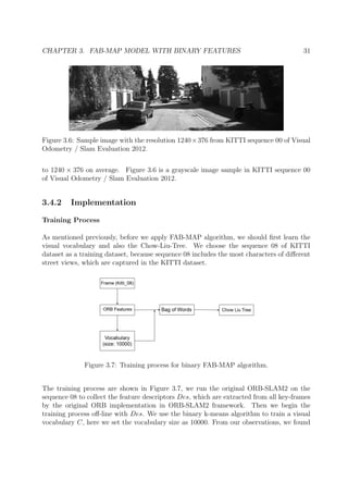
Kitti 07 4.994 ms 50.820 ms](https://image.slidesharecdn.com/c23b7113-893c-4f39-bb28-73befa7b3431-161213205645/85/Master_Thesis_Jiaqi_Liu-39-320.jpg)
![CHAPTER 3. FAB-MAP MODEL WITH BINARY FEATURES 35
0
100
200
300
400
500
-300 -200 -100 0 100 200 300
z[m]
x [m]
Ground Truth
Visual Odometry
Sequence Start
Loops
(a) ORB-SLAM2
0
100
200
300
400
500
-300 -200 -100 0 100 200 300
z[m]
x [m]
Ground Truth
Visual Odometry
Sequence Start
Loops
(b) Binary FAB-MAP
Figure 3.10: Comparison of robot trajectory in KITTI 00 between ORB-SLAM2 and Bi-
nary FAB-MAP
-100
0
100
200
300
400
-200 -100 0 100 200
z[m]
x [m]
Ground Truth
Visual Odometry
Sequence Start
Loops
(a) ORB-SLAM2
-100
0
100
200
300
400
-200 -100 0 100 200
z[m]
x [m]
Ground Truth
Visual Odometry
Sequence Start
Loops
(b) Binary FAB-MAP
Figure 3.11: Comparison of robot trajectory in KITTI 05 between ORB-SLAM2 and Bi-
nary FAB-MAP](https://image.slidesharecdn.com/c23b7113-893c-4f39-bb28-73befa7b3431-161213205645/85/Master_Thesis_Jiaqi_Liu-40-320.jpg)
![CHAPTER 3. FAB-MAP MODEL WITH BINARY FEATURES 36
-100
0
100
200
300
-200 -100 0 100 200
z[m]
x [m]
Ground Truth
Visual Odometry
Sequence Start
Loops
(a) ORB-SLAM2
-100
0
100
200
300
-200 -100 0 100 200
z[m]
x [m]
Ground Truth
Visual Odometry
Sequence Start
Loops
(b) Binary FAB-MAP
Figure 3.12: Comparison of robot trajectory in KITTI 06 between ORB-SLAM2 and Bi-
nary FAB-MAP
-50
0
50
100
-200 -150 -100 -50 0
z[m]
x [m]
Ground Truth
Visual Odometry
Sequence Start
Loops
(a) ORB-SLAM2
-50
0
50
100
-200 -150 -100 -50 0
z[m]
x [m]
Ground Truth
Visual Odometry
Sequence Start
Loops
(b) Binary FAB-MAP
Figure 3.13: Comparison of robot trajectory in KITTI 07 between ORB-SLAM2 and Bi-
nary FAB-MAP](https://image.slidesharecdn.com/c23b7113-893c-4f39-bb28-73befa7b3431-161213205645/85/Master_Thesis_Jiaqi_Liu-41-320.jpg)
![Chapter 4
VLAD Model with Binary Features
This chapter introduces an alternative compact image representation VLAD to replace
BoW. Similar to BoW, it is also a high dimensional vector generated from local descrip-
tors. However, each visual word in VLAD vector not only identifies the existence of one
cluster, but also contains the difference information between real descriptors and the clus-
ter centroids. According to the work [JDSP10], VLAD can achieve the same performance
as BoW with a smaller size. Moreover, to further reduce dimension of VLAD vector,
principal component analysis (PCA) [Bis06] can be applied in different stages of signature
generation. In the following sections, we will introduce the basic theory of different type
VLAD representations and the implementation for loop closure detection.
4.1 VLAD
4.1.1 VLAD Computation
Similar to BoW, before computing VLAD signature, a vocabulary C = {c1, ..., ck} based
on a collection of local descriptors is learned by a clustering algorithm (normally k-means),
where ci is a visual word which represents a cluster and k is the number of visual words.
For the local descriptor x, a nearest neighbor search is applied to find its visual word
ci = NN(x) and label it with the corresponding cluster index. Next, in each cluster
the differences x − ci between every descriptor with cluster label i and ci are computed,
subsequently accumulated to generate a residual vector.
Assume vi denotes one element of the VLAD signature, the computation process can be
expressed as following [JDSP10]:
vi =
x:NN(x)=ci
x − ci. (4.1)](https://image.slidesharecdn.com/c23b7113-893c-4f39-bb28-73befa7b3431-161213205645/85/Master_Thesis_Jiaqi_Liu-43-320.jpg)
![CHAPTER 4. VLAD MODEL WITH BINARY FEATURES 39
However, each individual local descriptor in one cluster does not provide the same contribu-
tion to the generation of a VLAD visual word. Therefore, in order to make all descriptors
contribute equally to the summation, the Equation 4.1 is adjusted as following [DGJP13]:
vi =
x:NN(x)=ci
x − ci
x − ci
. (4.2)
Subsequently, two normalizations are applied on the VLAD signature to make an improve-
ment. The first one is power normalization [PSM10] which is a non-linear process applied
on each visual word vi.
vi = |vi|α
× sign(vi), (4.3)
where 0 ≤ α < 1 is a normalization parameter. At last the whole VLAD vector is L2-
normalized:
v :=
v
v
. (4.4)
4.1.2 Local Coordinate System (LCS) PCA
In practical applications, there may be limitations of memory usage. It is therefore neces-
sary to reduce the dimension of VLAD signature while preserving the reliable performance.
To deal with this, Delhumeau, et al. [DGJP13] proposed a PCA scheme in a local coor-
dinate, which is called LCS-PCA. Usually, PCA is applied for the whole descriptor space.
However, in this case the first eigenvectors can’t capture various bursty patterns. Thus,
in order to obtain a better handling of burstiness, PCA is applied for each residual vector
corresponds to the visual word ci before aggregation and the rotation matrix Ri should be
learned off-line based on a training dataset. So the Equation 4.2 is adjusted as
vi =
x:NN(x)=ci
Ri
x − ci
x − ci
. (4.5)
However, in a real-time SLAM system, the average number of local descriptors ranges
from 1000 to 3000 per image. To deal with this number of descriptors, LCS-PCA has a
relative high computation complexity. In addition, the power normalization mentioned
in the section 4.1.1 is applied to the vector after aggregation. It is therefore better to
employ PCA on the aggregated residual vectors [ERL14]. So we apply the LCS-PCA to
the residual vectors after aggregation instead, which is more efficient than original design
and also performs well. Moreover, we also employ a whitening process on the rotation
matrices to average energy among the selected eigenvectors, which results in a better
performance [JC12]. Now Equation 4.5 is replaced by
vi = Rwi
x:NN(x)=ci
x − ci
x − ci
, (4.6)](https://image.slidesharecdn.com/c23b7113-893c-4f39-bb28-73befa7b3431-161213205645/85/Master_Thesis_Jiaqi_Liu-44-320.jpg)
![CHAPTER 4. VLAD MODEL WITH BINARY FEATURES 40
where Rwi is the rotation matrix for i-th cluster after whitening.
The vector v of size k × d is the VLAD signature, here k denotes the size of vocabulary
and d denotes the feature descriptor dimension after the adjusted LCS-PCA. If Rwi = I,
then no LCS-PCA is applied, and v is a k×d vector which is the original VLAD signature.
4.1.3 Signature Matching
In our approach, we need a matching score between two VLAD signatures to justify if the
compared two frames are extracted from a same location. The direct way is to measure
the similarity of different VLAD signatures. Assuming v and v are two VLAD signatures,
the similarity is defined as below:
Sim(v, v ) =
k
i=1 σ(vi, vi)
k
, (4.7)
where σ(vi, vi) is a match kernel. For the original VLAD signature, we set this kernel as
L2 distance between two representations.
4.2 Hierarchical Multi-VLAD
In a SLAM system for large-scale environment, it is time-consuming to detect loop closure
as the number of map points increases. So developing an efficient pre-filtering scheme is
necessary. Based on the work [WDL+
15] by Wang, et al. we realize an early rejection of
unlikely loop candidates by using short VLAD signature and verify the true loop candidates
with long one. In this section, the mathematical principle of hierarchical multi-VLAD is
introduced.
4.2.1 Multi-VLAD Representation
Similar to VLAD signature, in order to compute the multi-VLAD signatures, a tree-
structured hierarchical vocabulary is needed, which is illustrated in Figure 4.1. We assume
Tn
denotes the hierarchical vocabulary tree, where n is the depth of the tree. This vocabu-
lary tree also need to be learned off-line by hierarchical clustering algorithms (hierarchical
k-means). The nodes at j-th level is denoted as Cj
= {cj
1, ..., cj
kj } and kj
is the number
of nodes at j-th level, each node cj
i is the cluster centroid. In the computation process, a
local descriptor x moves from the root of Tn
to one node at next level, and at j-th level
the nearest neighbor cj
i of x is found, subsequently x is passed down to a child node of cj
i ,
and at the level j + 1 the same process is repeated until x reaches one leaf node of Tn
. At](https://image.slidesharecdn.com/c23b7113-893c-4f39-bb28-73befa7b3431-161213205645/85/Master_Thesis_Jiaqi_Liu-45-320.jpg)
![CHAPTER 4. VLAD MODEL WITH BINARY FEATURES 41
short vocabulary
long vocabulary
Figure 4.1: Tree-Structured Hierarchical Vocabulary
last, the residual vectors are calculated based on the compared nodes at each level, then
concatenated as a VLAD signature.
As mentioned previously, we need different sizes of VLAD signatures to realize loop closure
detection, which means at each level of Tn
a VLAD signature is generated independently.
So for the tree Tn
with depth n, there are n VLAD signatures vm = {vj
|j = 1, 2, ..., n},
where vj
= vj
1, ..., vj
kj is the signature generated at j-th level with the process described
above. So the algorithm can be expressed by
vj
i =
x:NNj(x)=cj
i
x − cj
i . (4.8)
4.2.2 Signature Matching
In the work [WDL+
15], the original design is to accumulate the weighted similarity of
the whole multi-VLAD signatures. Assume vm = {vj
|j = 1, 2, ..., n} and vm = {v j
|j =
1, 2, ..., n} are two multi-VLAD signatures, the similarity is defined as:
Simm(vm, vm) =
n
j=1
Sim(vj
, v j
)αj
, (4.9)
where Sim() is the similarity function defined in Equation 4.7 and αj is a weighting factor
for j-th level.
However, in our approach we need to compute the similarity score for each level indepen-
dently, which realizes different functions. For example, we want to use the similarity score
for short signatures to reject the most unlikely loop candidates, and use the similarity
score for long signatures to verify the true loop candidates. Thus, our similarity equation
is defined as following:
Sims∈{short,long}(v, v ) = Sim(vs
, v s
), (4.10)
where s identifies short or long signature we want to use.](https://image.slidesharecdn.com/c23b7113-893c-4f39-bb28-73befa7b3431-161213205645/85/Master_Thesis_Jiaqi_Liu-46-320.jpg)
![CHAPTER 4. VLAD MODEL WITH BINARY FEATURES 42
4.3 Product Quantization
4.3.1 Product Quantization Theory
The place recognition problem can be simplified as an image matching problem. It is
therefore necessary to find a fast image matching algorithm to accelerate the loop closure
detection process. J´egou et al. [JDS11] proposed a so-called product quantization scheme
combined with inverted index searching method to make image matching more efficient.
The basic idea of the product quantization is to group a fixed number of components in
one vector as subvectors, then each subvector is quantized separately.
Assuming v denotes the input vector, and it is divided as k subvectors ui with 1 ≤ i ≤ k.
We define the original dimension of v is d∗
and the dimension of one subvector is d which has
the relationship d = d∗
/k. Subsequently, these subvectors are quantized by k independent
quantizers. The vector is then mapped as following:
v1, ..., vd
u1
, ..., vd∗−d+1, ..., vd∗
uk
→ qz1(u1), ..., qzk(uk), (4.11)
where qzi is the quantizer for the i-th subvector, which possesses a codebook Qi and an
index set Ii.
So the final representation after product quantization is an index set of Cartesian product:
I = I1 × ... × Ik, (4.12)
which corresponds to a codebook set:
Q = Q1 × ... × Qk. (4.13)
In our case, k is the number of clusters for generating VLAD representation and the
subvector ui = vi, which is one residual vector of the VLAD signature. The size d is the
dimension of one residual vector.
4.3.2 Distance Computation
There are two different similarity measurements for the vector after product quantiza-
tion, SDC and ADC [JDS11]. Both measure the similarity by computing an approximate
distance between vectors.
Symmetric Distance Computation (SDC)
Given two VLAD signatures v and v , after product quantization they are represented
by the cluster centroids qz(v) and qz(v ). Now the distance d(v, v ) is approximated by](https://image.slidesharecdn.com/c23b7113-893c-4f39-bb28-73befa7b3431-161213205645/85/Master_Thesis_Jiaqi_Liu-47-320.jpg)
![CHAPTER 4. VLAD MODEL WITH BINARY FEATURES 43
d(qz(v), qz(v )), which can be expressed as follows:
d(v, v ) ≈ d(qz(v), qz(v )) =
k
i=1
d(qzi(vi), qzi(vi))2, (4.14)
where d(qzi(vi), qzi(vi))2
is computed by the difference of corresponding centroid pair
d(qil, qil )2
in the i-th quantizer, where l and l identify the index of the used represent
descriptor in Qi.
Asymmetric Distance Computation (ADC)
In this case, one VLAD signature v is quantized as qz(v ) and the other one v preserves
the original form. Now the distance d(v, v ) is approximated by d(v, qz(v )), which is
computed as following:
d(v, v ) ≈ d(v, qz(v )) =
k
i=1
d(vi, qzi(vi))2, (4.15)
where d(vi, qzi(vi))2
is calculated by d(vi, qil)2
and vi is i-th residual vector in v.
4.3.3 Inverted Index Searching
For image matching, it is very efficient to apply an inverted file system [SZ03] in real-time
applications. Thus, based on the work [JDS11], we also apply an inverted file system with
asymmetric distance computation (IVFADC) to accelerate the VLAD matching process.
The computation of the inverted index vector based on VLAD signature can be divided
into two parts: training and searching. Figure 4.2 can be treated as an example.
Training
Similar to VLAD computation, at first we need to train a vocabulary C of size k. Then we
repeat the same computation process for VLAD to get the signatures for all images of the
training dataset. In addition, for each visual word vi a product quantization codebook Qi
of size m based on i-th residual vectors is also trained, as shown in Figure 4.2.](https://image.slidesharecdn.com/c23b7113-893c-4f39-bb28-73befa7b3431-161213205645/85/Master_Thesis_Jiaqi_Liu-48-320.jpg)
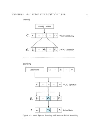
![CHAPTER 4. VLAD MODEL WITH BINARY FEATURES 45
Searching
For a new image imported into the system, we first extract the local descriptors Des.
Then a VLAD signature v is generated from Des with the vocabulary C. Subsequently,
a nearest neighbor search in the codebook Qi is applied. If NN(vi) = qil, then the i-th
element Ii in the final index vector is assigned as an integer index l. We repeat this process
until all k visual words are represented by the index of its nearest neighbor, then the final
index vector is generated. Because this vector only contains k integer values range from
1 to m, it is very efficient for image matching, which is suitable for loop closure detection
combined with the VLAD signature in a real-time SLAM.
4.4 Experiment
Similar to the experiment for binary FAB-MAP, in order to evaluate the performance of
different algorithms based on the VLAD representations, we implement the corresponding
loop closure detection method to replace the original one in ORB-SLAM2 framework. The
ORB-SLAM2 with new loop closure detection algorithms is tested in stereo mode on a
computer with 8GB RAM and an Intel Core i5-3600HQ running at 2.30GHZ. The KITTI
sequences 00, 05, 06 and 07 [GLU12] are still treated as our test datasets. The detail
information of KITTI dataset is introduced in section 3.4.1. The results are accepted if at
least 5 continuous runs are successful. In the following sections, we use VLAD to denote
the original VLAD signature, HMVLAD to denote hierarchical multi-VLAD signatures
and VLAD+PQ to denote the VLAD signature with the product quantization scheme.
Moreover, in order to make the image matching more efficient, we binarized the VLAD and
HMVLAD signatures. Thus, for similarity measurement, Hamming distance is calculated.
All the implementation details are introduced in the following section.
4.4.1 Implementation
Training Process
Similar to BoW, before we compute VLAD representations, we should first learn the visual
vocabulary. We still choose the sequence 08 of KITTI as a training dataset, in order to
compare different algorithms based on the same conditions.
As illustrated in Figure 4.3, the training process is made off-line based on the feature
descriptors, which have been already extracted for the experiment of binary FAB-MAP.
For different kinds of representations, we should train different vocabularies. For VLAD
signature, we used the ORB features of key-frames to train a vocabulary C of size 4.
In addition, for VLAD+PQ signature, we furthermore trained the independent product](https://image.slidesharecdn.com/c23b7113-893c-4f39-bb28-73befa7b3431-161213205645/85/Master_Thesis_Jiaqi_Liu-50-320.jpg)
![CHAPTER 4. VLAD MODEL WITH BINARY FEATURES 46
quantization codebooks with size 32 for each visual word in C. And we trained a two
level tree-structured hierarchical vocabulary, whose sizes are 2 and 4 at each level. In the
training process we can also set the LCS-PCA dimensions, but during our experiments we
don’t suffer from the lack of memory, so we use no LCS-PCA.
Figure 4.3: Training process for VLAD representations
Loop Closure Detection with VLAD in ORB-SLAM2
At first we want to evaluate the loop detection performance by VLAD signature without
any pre-filter technique. This approach serves as the baseline for the improvement in the
following two sections. Without any pre-filtering mechanism, more loop closure detection
time is required for large-scale datasets like KITTI 00. So the performance of this imple-
mentation is treated as the ”worst case” among all three algorithms, which provides us a
clear reference standard for future improvement.
We assume the current key-frame is denoted as K, and firstly we compute the Hamming
distances as a similarity score S between signatures of K and its each neighbor in convisi-
bility graph [MAMT15]. Then a minimal score minS is found in between. Subsequently,
we continue to compute the similarity score S for each previous key-frame which doesn’t
connect to K through the covisibility graph. If one previous key-frame obtains a smaller
score than minS, then this key-frame is identified as a loop candidate of K. The whole
process is illustrated in Figure 4.4.](https://image.slidesharecdn.com/c23b7113-893c-4f39-bb28-73befa7b3431-161213205645/85/Master_Thesis_Jiaqi_Liu-51-320.jpg)

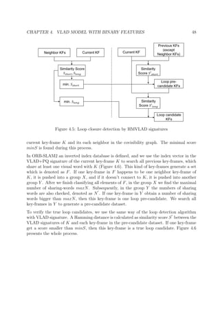
![CHAPTER 4. VLAD MODEL WITH BINARY FEATURES 49
Figure 4.6: Loop closure detection by VLAD+PQ signatures
4.4.2 Performance Evaluation
We use the same criteria for binary FAB-MAP to evaluate the performance: robot trajec-
tory and average loop closure detection time. In addition, for the second criterion we also
measure the timings for each loop in all four datasets [MAMT15]. This measurement can
provide a detail view for the efficiency and accuracy of every algorithm. Both criteria are
compared with the original loop closure detection method in ORB-SLAM2.
Robot Trajectory
Similar to the experiment for binary FAB-MAP, we compare the robot trajectories
among the four loop detection methods by using original HBoW, VLAD, HMVLAD and
VLAD+PQ. Figure 4.7 to Figure 4.10 show the comparisons of robot trajectories for se-
quence 00, 05, 06 and 07 of KITTI dataset. The red line shows the ground truth and the
blue dash line shows the trajectory produced from a SLAM system. In addition, the green
circles identify the location where a loop is detected. From this result, we can observe
that all four approaches provide accurate loop detections. All loops are detected and the
loops are detected almost at the same location. Based on this result we can conclude
that the algorithms based on the VLAD representations with binary features provide good
performance for loop closure detection.](https://image.slidesharecdn.com/c23b7113-893c-4f39-bb28-73befa7b3431-161213205645/85/Master_Thesis_Jiaqi_Liu-54-320.jpg)
![CHAPTER 4. VLAD MODEL WITH BINARY FEATURES 50
0
100
200
300
400
500
-300 -200 -100 0 100 200 300
z[m]
x [m]
Ground Truth
Visual Odometry
Sequence Start
Loops
(a) ORB-SLAM2
0
100
200
300
400
500
-300 -200 -100 0 100 200 300
z[m]
x [m]
Ground Truth
Visual Odometry
Sequence Start
Loops
(b) VLAD
0
100
200
300
400
500
-300 -200 -100 0 100 200 300
z[m]
x [m]
Ground Truth
Visual Odometry
Sequence Start
Loops
(c) HMVLAD
0
100
200
300
400
500
-300 -200 -100 0 100 200 300
z[m]
x [m]
Ground Truth
Visual Odometry
Sequence Start
Loops
(d) VLAD+PQ
Figure 4.7: Comparison of robot trajectory in KITTI 00 among ORB-SLAM2, VLAD,
HMVLAD and VLAD+PQ](https://image.slidesharecdn.com/c23b7113-893c-4f39-bb28-73befa7b3431-161213205645/85/Master_Thesis_Jiaqi_Liu-55-320.jpg)
![CHAPTER 4. VLAD MODEL WITH BINARY FEATURES 51
-100
0
100
200
300
400
-200 -100 0 100 200
z[m]
x [m]
Ground Truth
Visual Odometry
Sequence Start
Loops
(a) ORB-SLAM2
-100
0
100
200
300
400
-200 -100 0 100 200
z[m]
x [m]
Ground Truth
Visual Odometry
Sequence Start
Loops
(b) VLAD
-100
0
100
200
300
400
-200 -100 0 100 200
z[m]
x [m]
Ground Truth
Visual Odometry
Sequence Start
Loops
(c) HMVLAD
-100
0
100
200
300
400
-200 -100 0 100 200
z[m]
x [m]
Ground Truth
Visual Odometry
Sequence Start
Loops
(d) VLAD+PQ
Figure 4.8: Comparison of robot trajectory in KITTI 05 among ORB-SLAM2, VLAD,
HMVLAD and VLAD+PQ](https://image.slidesharecdn.com/c23b7113-893c-4f39-bb28-73befa7b3431-161213205645/85/Master_Thesis_Jiaqi_Liu-56-320.jpg)
![CHAPTER 4. VLAD MODEL WITH BINARY FEATURES 52
-100
0
100
200
300
-200 -100 0 100 200
z[m]
x [m]
Ground Truth
Visual Odometry
Sequence Start
Loops
(a) ORB-SLAM2
-100
0
100
200
300
-200 -100 0 100 200
z[m]
x [m]
Ground Truth
Visual Odometry
Sequence Start
Loops
(b) VLAD
-100
0
100
200
300
-200 -100 0 100 200
z[m]
x [m]
Ground Truth
Visual Odometry
Sequence Start
Loops
(c) HMVLAD
-100
0
100
200
300
-200 -100 0 100 200
z[m]
x [m]
Ground Truth
Visual Odometry
Sequence Start
Loops
(d) VLAD+PQ
Figure 4.9: Comparison of robot trajectory in KITTI 06 among ORB-SLAM2, VLAD,
HMVLAD and VLAD+PQ](https://image.slidesharecdn.com/c23b7113-893c-4f39-bb28-73befa7b3431-161213205645/85/Master_Thesis_Jiaqi_Liu-57-320.jpg)
![CHAPTER 4. VLAD MODEL WITH BINARY FEATURES 53
-50
0
50
100
-200 -150 -100 -50 0
z[m]
x [m]
Ground Truth
Visual Odometry
Sequence Start
Loops
(a) ORB-SLAM2
-50
0
50
100
-200 -150 -100 -50 0
z[m]
x [m]
Ground Truth
Visual Odometry
Sequence Start
Loops
(b) VLAD
-50
0
50
100
-200 -150 -100 -50 0
z[m]
x [m]
Ground Truth
Visual Odometry
Sequence Start
Loops
(c) HMVLAD
-50
0
50
100
-200 -150 -100 -50 0
z[m]
x [m]
Ground Truth
Visual Odometry
Sequence Start
Loops
(d) VLAD+PQ
Figure 4.10: Comparison of robot trajectory in KITTI 07 among ORB-SLAM2, VLAD,
HMVLAD and VLAD+PQ](https://image.slidesharecdn.com/c23b7113-893c-4f39-bb28-73befa7b3431-161213205645/85/Master_Thesis_Jiaqi_Liu-58-320.jpg)


![List of Figures
1.1 Example of SLAM structure. The Loop Closure block is the concern of this
thesis. . . . . . . . . . . . . . . . . . . . . . . . . . . . . . . . . . . . . . . 2
1.2 Different observations from the same location at different time points. The
feature points are extracted by FAST detector. . . . . . . . . . . . . . . . . 4
1.3 Observations from two different locations with distance 100m. The feature
points are extracted by FAST detector. . . . . . . . . . . . . . . . . . . . 4
2.1 Bag of Words for image clustering [Li11]. . . . . . . . . . . . . . . . . . . . 13
2.2 VLAD signature generation. Here, c represents the cluster centroid, x is a
new local descriptor and v is one residual vector which is one component of
the final VLAD signature [Li15]. . . . . . . . . . . . . . . . . . . . . . . . . 14
2.3 ORB-SLAM system overview, showing the tracking, local mapping and loop
closing threads. The place recognition module and the map are also illus-
trated. Adapted from [MAMT15]. . . . . . . . . . . . . . . . . . . . . . . . 16
2.4 Tracking Thread in ORB-SLAM2. . . . . . . . . . . . . . . . . . . . . . . . 18
2.5 Local Mapping Thread in ORB-SLAM2. . . . . . . . . . . . . . . . . . . . 19
2.6 Loop Closing Thread in ORB-SLAM2. . . . . . . . . . . . . . . . . . . . . 20
3.1 Left: Graph of the underlying distribution P(Z). The edges are weighted
by mutual information between variables. The edges that contribute to the
maximal sum of branch weights are shown by the solid lines. Middle: Naive
Bayes approximation. Right: Chow-Liu-Tree [CN08]. . . . . . . . . . . . . 23
3.2 Naive Bayes Model. Adapted from [CN08]. . . . . . . . . . . . . . . . . . . 25
3.3 Chow Liu Model. Adapted from [CN08]. . . . . . . . . . . . . . . . . . . . 26
3.4 Intuitive Model. Adapted from [CN08]. . . . . . . . . . . . . . . . . . . . . 27
3.5 FAB-MAP Model. Adapted from [CN08]. . . . . . . . . . . . . . . . . . . . 28
3.6 Sample image with the resolution 1240 × 376 from KITTI sequence 00 of
Visual Odometry / Slam Evaluation 2012. . . . . . . . . . . . . . . . . . . 31
3.7 Training process for binary FAB-MAP algorithm. . . . . . . . . . . . . . . 31
3.8 Binary Expansion. b is the bit representation and B is the byte representation. 32
3.9 Pre-filtering process for FAB-MAP algorithm. The red O is the offset for
L2 distance. . . . . . . . . . . . . . . . . . . . . . . . . . . . . . . . . . . . 33
58](https://image.slidesharecdn.com/c23b7113-893c-4f39-bb28-73befa7b3431-161213205645/85/Master_Thesis_Jiaqi_Liu-63-320.jpg)

![List of Tables
2.1 Average computation time over 24 640×480 images from the Pascal dataset
[RRKB11,EVGW+
10] . . . . . . . . . . . . . . . . . . . . . . . . . . . . . 11
3.1 Average time for representation creation . . . . . . . . . . . . . . . . . . . 34
3.2 Average loop candidate detection time per key-frame . . . . . . . . . . . . 34
4.1 Average time for signature creation . . . . . . . . . . . . . . . . . . . . . . 54
4.2 Average loop candidate detection time per key-frame . . . . . . . . . . . . 54
4.3 Comparison of timing per loop in KITTI 00 among HBoW, VLAD,
HMVLAD and VLAD+PQ. . . . . . . . . . . . . . . . . . . . . . . . . . . 55
4.4 Comparison of timing per loop in KITTI 05 among HBoW, VLAD,
HMVLAD and VLAD+PQ. . . . . . . . . . . . . . . . . . . . . . . . . . . 55
4.5 Comparison of timing per loop in KITTI 06 among HBoW, VLAD,
HMVLAD and VLAD+PQ. . . . . . . . . . . . . . . . . . . . . . . . . . . 56
4.6 Comparison of timing per loop in KITTI 07 among HBoW, VLAD,
HMVLAD and VLAD+PQ. . . . . . . . . . . . . . . . . . . . . . . . . . . 56
60](https://image.slidesharecdn.com/c23b7113-893c-4f39-bb28-73befa7b3431-161213205645/85/Master_Thesis_Jiaqi_Liu-65-320.jpg)


![Bibliography
[BETVG08] Herbert Bay, Andreas Ess, Tinne Tuytelaars, and Luc Van Gool. Speeded-
up robust features (surf). Computer vision and image understanding,
110(3):346–359, 2008.
[Bis06] Christopher M Bishop. Pattern recognition. Machine Learning, 128, 2006.
[BMM07] Anna Bosch, Xavier Mu˜noz, and Robert Mart´ı. Which is the best way to
organize/classify images by content? Image and vision computing, 25(6):778–
791, 2007.
[Bro59] David T Brown. A note on approximations to discrete probability distribu-
tions. Information and Control, 2(4):386–392, 1959.
[BSLK04] Yaakov Bar-Shalom, X Rong Li, and Thiagalingam Kirubarajan. Estimation
with applications to tracking and navigation: theory algorithms and software.
John Wiley & Sons, 2004.
[CL68] C Chow and C Liu. Approximating discrete probability distributions with
dependence trees. IEEE transactions on Information Theory, 14(3):462–467,
1968.
[CLSF10] Michael Calonder, Vincent Lepetit, Christoph Strecha, and Pascal Fua. Brief:
Binary robust independent elementary features. In European conference on
computer vision, pages 778–792. Springer, 2010.
[CN08] Mark Cummins and Paul Newman. Fab-map: Probabilistic localization and
mapping in the space of appearance. The International Journal of Robotics
Research, 27(6):647–665, 2008.
[Cum09] Mark Cummins. Probabilistic Localization and Mapping in Appearance Space.
PhD thesis, University of Oxford, 2009.
[DGJP13] Jonathan Delhumeau, Philippe-Henri Gosselin, Herv´e J´egou, and Patrick
P´erez. Revisiting the vlad image representation. In Proceedings of the 21st
ACM international conference on Multimedia, pages 653–656. ACM, 2013.
63](https://image.slidesharecdn.com/c23b7113-893c-4f39-bb28-73befa7b3431-161213205645/85/Master_Thesis_Jiaqi_Liu-68-320.jpg)
![BIBLIOGRAPHY 64
[DSSS04] Roman Dementiev, Peter Sanders, Dominik Schultes, and Jop Sibeyn. Engi-
neering an external memory minimum spanning tree algorithm. In Exploring
New Frontiers of Theoretical Informatics, pages 195–208. Springer, 2004.
[ED08] Ethan Eade and Tom Drummond. Unified loop closing and recovery for real
time monocular slam. In BMVC, volume 13, page 136, 2008.
[ERL14] Christian Eggert, Stefan Romberg, and Rainer Lienhart. Improving vlad:
Hierarchical coding and a refined local coordinate system. In ICIP, pages
3018–3022, 2014.
[ESC14] Jakob Engel, Thomas Sch¨ops, and Daniel Cremers. Lsd-slam: Large-scale
direct monocular slam. In European Conference on Computer Vision, pages
834–849. Springer, 2014.
[EVGW+
10] Mark Everingham, Luc Van Gool, Christopher KI Williams, John Winn,
and Andrew Zisserman. The pascal visual object classes (voc) challenge.
International journal of computer vision, 88(2):303–338, 2010.
[GLSU13] Andreas Geiger, Philip Lenz, Christoph Stiller, and Raquel Urtasun. Vision
meets robotics: The kitti dataset. The International Journal of Robotics
Research, page 0278364913491297, 2013.
[GLT12] Dorian G´alvez-L´opez and Juan D Tardos. Bags of binary words for fast place
recognition in image sequences. IEEE Transactions on Robotics, 28(5):1188–
1197, 2012.
[GLU12] Andreas Geiger, Philip Lenz, and Raquel Urtasun. Are we ready for au-
tonomous driving? the kitti vision benchmark suite. In Computer Vision
and Pattern Recognition (CVPR), 2012 IEEE Conference on, pages 3354–
3361. IEEE, 2012.
[Hor87] Berthold KP Horn. Closed-form solution of absolute orientation using unit
quaternions. JOSA A, 4(4):629–642, 1987.
[JC12] Herv´e J´egou and Ondˇrej Chum. Negative evidences and co-occurences in
image retrieval: The benefit of pca and whitening. In Computer Vision–
ECCV 2012, pages 774–787. Springer, 2012.
[JDS11] Herve Jegou, Matthijs Douze, and Cordelia Schmid. Product quantization for
nearest neighbor search. IEEE transactions on pattern analysis and machine
intelligence, 33(1):117–128, 2011.
[JDSP10] Herv´e J´egou, Matthijs Douze, Cordelia Schmid, and Patrick P´erez. Aggre-
gating local descriptors into a compact image representation. In Computer
Vision and Pattern Recognition (CVPR), 2010 IEEE Conference on, pages
3304–3311. IEEE, 2010.](https://image.slidesharecdn.com/c23b7113-893c-4f39-bb28-73befa7b3431-161213205645/85/Master_Thesis_Jiaqi_Liu-69-320.jpg)
![BIBLIOGRAPHY 65
[JGJS99] Michael I Jordan, Zoubin Ghahramani, Tommi S Jaakkola, and Lawrence K
Saul. An introduction to variational methods for graphical models. Machine
learning, 37(2):183–233, 1999.
[JU97] Simon J Julier and Jeffrey K Uhlmann. New extension of the kalman filter
to nonlinear systems. In AeroSense’97, pages 182–193. International Society
for Optics and Photonics, 1997.
[Kal60] Rudolph Emil Kalman. A new approach to linear filtering and prediction
problems. Journal of basic Engineering, 82(1):35–45, 1960.
[KL51] Solomon Kullback and Richard A Leibler. On information and sufficiency.
The annals of mathematical statistics, 22(1):79–86, 1951.
[KM07] Georg Klein and David Murray. Parallel tracking and mapping for small ar
workspaces. In Mixed and Augmented Reality, 2007. ISMAR 2007. 6th IEEE
and ACM International Symposium on, pages 225–234. IEEE, 2007.
[KM08] Georg Klein and David Murray. Improving the agility of keyframe-based slam.
In European Conference on Computer Vision, pages 802–815. Springer, 2008.
[Lew59] PM Lewis. Approximating probability distributions to reduce storage re-
quirements. Information and control, 2(3):214–225, 1959.
[LF06] Vincent Lepetit and Pascal Fua. Keypoint recognition using randomized
trees. IEEE transactions on pattern analysis and machine intelligence,
28(9):1465–1479, 2006.
[LFP11] Jongwoo Lim, Jan-Michael Frahm, and Marc Pollefeys. Online environment
mapping. In Computer Vision and Pattern Recognition (CVPR), 2011 IEEE
Conference on, pages 3489–3496. IEEE, 2011.
[Li11] Fei-Fei Li. Object recognition: Bag of words models & part-based gen-
erative models, 2011. http://vision.stanford.edu/teaching/cs231a_
autumn1112/lecture/lecture15_bow_part-based_cs231a_marked.pdf.
[Li15] Zhu Li. Feature aggregation: Bag of words, vlad, fisher vector, and
akula, 2015. http://l.web.umkc.edu/lizhu/teaching/ee401.2015fa.
multimedia-analysis/notes/lec07-Aggregation-BoW-VLAD-1.2.pdf.
[LMNF09] Vincent Lepetit, Francesc Moreno-Noguer, and Pascal Fua. Epnp: An ac-
curate o (n) solution to the pnp problem. International journal of computer
vision, 81(2):155–166, 2009.
[Low99] David G Lowe. Object recognition from local scale-invariant features. In
Computer vision, 1999. The proceedings of the seventh IEEE international
conference on, volume 2, pages 1150–1157. Ieee, 1999.](https://image.slidesharecdn.com/c23b7113-893c-4f39-bb28-73befa7b3431-161213205645/85/Master_Thesis_Jiaqi_Liu-70-320.jpg)
![BIBLIOGRAPHY 66
[MAMT15] Raul Mur-Artal, JMM Montiel, and Juan D Tard´os. Orb-slam: a versa-
tile and accurate monocular slam system. IEEE Transactions on Robotics,
31(5):1147–1163, 2015.
[MAT14] Ra´ul Mur-Artal and Juan D Tard´os. Fast relocalisation and loop closing in
keyframe-based slam. In 2014 IEEE International Conference on Robotics
and Automation (ICRA), pages 846–853. IEEE, 2014.
[MAT15] Ra´ul Mur-Artal and Juan D Tard´os. Probabilistic semi-dense mapping from
highly accurate feature-based monocular slam. Proceedings of Robotics: Sci-
ence and Systems, Rome, Italy, 1, 2015.
[Mei99] Marina Meila. An accelerated chow and liu algorithm: fitting tree distribu-
tions to high dimensional sparse data. 1999.
[MSDB03] M Michael, T Sebastian, K Daphne, and W Ben. Fastslam 2.0: An im-
proved particle filtering algorithm for simultaneous localization and mapping
that provably converges. In Proceedings of the Sixteenth International Joint
Conference on Artificial Intelligence (IJCAI), 2003.
[MTK+
02] Michael Montemerlo, Sebastian Thrun, Daphne Koller, Ben Wegbreit, et al.
Fastslam: A factored solution to the simultaneous localization and mapping
problem. In Aaai/iaai, pages 593–598, 2002.
[NLD11] Richard A Newcombe, Steven J Lovegrove, and Andrew J Davison. Dtam:
Dense tracking and mapping in real-time. In 2011 international conference
on computer vision, pages 2320–2327. IEEE, 2011.
[PRB10] Katrin Pirker, Matthias R¨uther, and Horst Bischof. Histogram of oriented
cameras-a new descriptor for visual slam in dynamic environments. In BMVC,
pages 1–12, 2010.
[PRB11] Katrin Pirker, Matthias R¨uther, and Horst Bischof. Cd slam-continuous lo-
calization and mapping in a dynamic world. In 2011 IEEE/RSJ International
Conference on Intelligent Robots and Systems, pages 3990–3997. IEEE, 2011.
[PSM10] Florent Perronnin, Jorge S´anchez, and Thomas Mensink. Improving the fisher
kernel for large-scale image classification. In European conference on computer
vision, pages 143–156. Springer, 2010.
[RD05] Edward Rosten and Tom Drummond. Fusing points and lines for high per-
formance tracking. In Tenth IEEE International Conference on Computer
Vision (ICCV’05) Volume 1, volume 2, pages 1508–1515. IEEE, 2005.
[Ros99] Paul L Rosin. Measuring corner properties. Computer Vision and Image
Understanding, 73(2):291–307, 1999.](https://image.slidesharecdn.com/c23b7113-893c-4f39-bb28-73befa7b3431-161213205645/85/Master_Thesis_Jiaqi_Liu-71-320.jpg)
![BIBLIOGRAPHY 67
[RRKB11] Ethan Rublee, Vincent Rabaud, Kurt Konolige, and Gary Bradski. Orb:
An efficient alternative to sift or surf. In 2011 International conference on
computer vision, pages 2564–2571. IEEE, 2011.
[SDMK11] Hauke Strasdat, Andrew J Davison, JMM Montiel, and Kurt Konolige. Dou-
ble window optimisation for constant time visual slam. In 2011 International
Conference on Computer Vision, pages 2352–2359. IEEE, 2011.
[SMD10] Hauke Strasdat, JMM Montiel, and Andrew J Davison. Scale drift-aware
large scale monocular slam. Robotics: Science and Systems VI, 2010.
[SSC90] Randall Smith, Matthew Self, and Peter Cheeseman. Estimating uncertain
spatial relationships in robotics. In Autonomous robot vehicles, pages 167–
193. Springer, 1990.
[SZ03] Josef Sivic and Andrew Zisserman. Video google: A text retrieval approach
to object matching in videos. In Computer Vision, 2003. Proceedings. Ninth
IEEE International Conference on, pages 1470–1477. IEEE, 2003.
[TLD+
13] Wei Tan, Haomin Liu, Zilong Dong, Guofeng Zhang, and Hujun Bao. Robust
monocular slam in dynamic environments. In Mixed and Augmented Reality
(ISMAR), 2013 IEEE International Symposium on, pages 209–218. IEEE,
2013.
[TMHF99] Bill Triggs, Philip F McLauchlan, Richard I Hartley, and Andrew W Fitzgib-
bon. Bundle adjustment-a modern synthesis. In International workshop on
vision algorithms, pages 298–372. Springer, 1999.
[WDL+
15] Yitong Wang, Ling-Yu Duan, Jie Lin, Zhe Wang, and Tiejun Huang. Hierar-
chical multi-vlad for image retrieval. In Image Processing (ICIP), 2015 IEEE
International Conference on, pages 4629–4633. IEEE, 2015.
[WKR11] Brian Williams, Georg Klein, and Ian Reid. Automatic relocalization and
loop closing for real-time monocular slam. IEEE transactions on pattern
analysis and machine intelligence, 33(9):1699–1712, 2011.](https://image.slidesharecdn.com/c23b7113-893c-4f39-bb28-73befa7b3431-161213205645/85/Master_Thesis_Jiaqi_Liu-72-320.jpg)


![[IJET-V1I6P1] Authors: Ms.Jare Dipali Y ,Ms.Khadse Shweta S ,Ms.Sawant Kalyan...](https://cdn.slidesharecdn.com/ss_thumbnails/ijet-v1i6p1-151121034138-lva1-app6892-thumbnail.jpg?width=640&height=640&fit=bounds)