1. Aalto University
School of Science
Degree Programme in Machine Learning and Data Mining
Miquel Perelló Nieto
Merging chrominance and luminance in
early, medium, and late fusion using
Convolutional Neural Networks
Master’s Thesis
Espoo, May 25, 2015
Supervisor: Prof. Tapani Raiko, Aalto University
Advisors: D.Sc. (Tech) Markus Koskela, University of Helsinki
Prof. Ricard Gavaldà Mestre, Universitat Politècnica de Catalunya
2.
3. Aalto University
School of Science
Degree Programme in Machine Learning and Data Mining
abstract of the
master’s thesis
Author: Miquel Perelló Nieto
Title: Merging chrominance and luminance in early, medium, and late fusion
using Convolutional Neural Networks
Date: 27.05.2015 Language: English Number of pages: 24+166
Professorship: Computer and Information Science Code: T-61
Supervisor: Prof. Tapani Raiko
Advisors: D.Sc. (Tech.) Markus Koskela, Prof. Ricard Gavaldà Mestre
The field of Machine Learning has received extensive attention in recent years.
More particularly, computer vision problems have got abundant consideration as
the use of images and pictures in our daily routines is growing.
The classification of images is one of the most important tasks that can be used
to organize, store, retrieve, and explain pictures. In order to do that, researchers
have been designing algorithms that automatically detect objects in images. Dur-
ing last decades, the common approach has been to create sets of features – man-
ually designed – that could be exploited by image classification algorithms. More
recently, researchers designed algorithms that automatically learn these sets of
features, surpassing state-of-the-art performances.
However, learning optimal sets of features is computationally expensive and it can
be relaxed by adding prior knowledge about the task, improving and accelerating
the learning phase. Furthermore, with problems with a large feature space the
complexity of the models need to be reduced to make it computationally tractable
(e.g. the recognition of human actions in videos).
Consequently, we propose to use multimodal learning techniques to reduce the
complexity of the learning phase in Artificial Neural Networks by incorporating
prior knowledge about the connectivity of the network. Furthermore, we analyze
state-of-the-art models for image classification and propose new architectures that
can learn a locally optimal set of features in an easier and faster manner.
In this thesis, we demonstrate that merging the luminance and the chrominance
part of the images using multimodal learning techniques can improve the acquisi-
tion of good visual set of features. We compare the validation accuracy of several
models and we demonstrate that our approach outperforms the basic model with
statistically significant results.
Keywords: Machine learning, computer vision, image classification, artificial
neural network, convolutional neural network, image processing,
Connectionism.
5. Preface
This thesis summarizes the work that I have been developing as a Master student on
my final research project in the Department of Information and Computer Science in
the Aalto Univeristy School of Science under the supervision of Prof. Tapani Raiko
and Dr. Markus Koskela, and the remote support from Prof. Ricard Gavaldà.
I would like to thank the discussions and comments about topics related to my
thesis to Vikram Kamath, Gerben van den Broeke, and Antti Rasmus. And for
general tips and advises during my studies to Ehsan Amid, Mathias Berglund, Pyry
Takala and Karmen Dykstra.
Finally, thanks to Jose C. Valencia Almansa for hi visits to Finland and his
company in a trip through Europe. And a special thank to Virginia Rodriguez
Almansa to believe in me and gave me support towards the acquisition of my Master
degree, moving to a foreign country for two years and studding abroad.
“All in all, thanks to everybody,
since without anybody this work
will make no sense”
— Miquel Perelló Nieto (2012)
Otaniemi, 27.05.2015
Miquel Perelló Nieto
v
7. A note from the author
After the completion of this thesis, further experiments seem to demonstrate that
it is possible to achieve the same validation accuracy by merging the chrominance
and the luminance in early fusion with similar number of parameters. However,
learning separate filters for the luminance and the chrominance achieved the same
performance, while showing a faster learning curve, better generalization and the
possibility of parallelize the training on different machines or graphics processor
units. Furthermore the results of this thesis are extensible to other sets of features
where the fusion level is not clear (e.g. audio, optical flow, captions, or other useful
features).
Otaniemi, 27.05.2015
Miquel Perelló Nieto
vii
13. Mathematical Notation
• This thesis contains some basic mathematical notes.
• I followed notation from [Bishop, 2006]
– Vectors: lower case Bold Roman column vector w or w = (w1, . . . , wM )
– Vectors: row vector is the transpose wT
or wT
= (w1, . . . , wM )T
– Matrices: Upper case Bold Roman M
– Closed interval: [a, b]
– Open interval: (a, b)
– Semi-closed interval: (a, b] and [a, b)
– Unit/identity matrix: of ize M × M is IM
xiii
25. Chapter 1
Introduction
“Do the difficult things while they are easy and
do the great things while they are small. A
journey of a thousand miles must begin with a
single step”
— Lao Tzu
Machine learning and artificial intelligence are two young fields of computer sci-
ence. However, their foundations are inherent in the understanding of intelligence,
and the best example of intelligence can be found in the brain. The comprehension
of the process of learning and the emergence of intelligence has been widely studied
since humans had the capability to hypothesize what other people think. Philoso-
phers, psychologists, sociologists, and physiologists, have attempted to solve these
type of questions. However, with the development of the first computers, engineers,
mathematicians, physicists and computer scientists started implementing the old
ideas on electronic devices. After years of developing new ideas – and improving
the computational power of these electronic devices – the terms machine learning
and artificial intelligence have gotten further attention; and actually got their name.
Nowadays, the tasks that researchers try to automate are usually very practical and
less theoretical. Nevertheless, the biggest changes come with unexpected theoretical
breakthroughs. Researchers explore new algorithms to solve important problems in
a large number of domains: path planning, decision making, optimal control, game
theory, regression, clustering, pattern recognition, information retrieval, logics, data
mining, and in multiple applications that – we hope – can be learned automatically.
In this thesis, we look at a narrow problem of pattern recognition in computer vision
– the image classification problem – and evaluate state-of-the-art models to extract
important conclusions that can help us to understand the process of vision. We
analyze and extend the previous work, in a desire to contribute in that manner to
the computer vision research community.
1
26. 2 CHAPTER 1. INTRODUCTION
1.1 Motivation
In the computer vision community, researchers have been trying to improve image
classification and object recognition algorithms since the late 80s. However, we still
do not know what is the optimal way to solve these problems. Despite the fact
that humans are able to solve these tasks from the early stages of our lives, we still
do not comprehend which are the features that we use to succeed. For us, colors
are a natural part of vision, but, the perception of colors is a subjective process
for each brain. Furthermore, there are animals that only perceive the environment
in a gray-scale of tones, while other animals can perceive ultra-light frequencies of
color. The requirements of the retinal photoreceptors have changed with evolution,
making different species to perceive a diverse number of colors.
One of the most basic vision systems is the perception of one unique light wave-
length. This is enough to perceive the luminance of the environment and determine
edges, shapes, blobs and other patterns. For example, nocturnal animals usually
have one type of photoreceptor and, therefore, can only see in a gray scale. The
luminance is one of the most important features to recognize objects and scenes,
while the perception of additional colors has been valuable to distinguish between
poisonous fruits, venomous animals, and other important situations.
Although we still do not know completely how our brain understands the envi-
ronment that we perceive, lately we have been able to train mathematical models
that learn to solve image classification tasks automatically. Earlier approaches tried
to create sets of hand-crafted features, usually driven by common sense or inspi-
ration from biology. However, during the last decade, researchers achieved very
good results by using mathematical models that learn to extract the sets of features
automatically. The resulting features could be astonishing, as they for example
discovered the importance of the luminance as an isolated feature, while the chromi-
nance seemed to have less importance (although it contains 2/3 parts of the total
information).
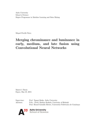
If we look at the initial filters that one of these models learned from a huge
number of images (see Figure 1.1a) we can see that more than half of the filters are
focused on the luminance, while the chrominance plays a secondary role for the image
classification task. If we visualize all the possible values that a pixel can have, the
gray-scale is only the diagonal of the resulting 3D cube. This small region in a cube
with 256 values per color correspond to a portion of 256/2563
= 1/2562
≈ 1.5×10⁻⁵
of the complete cube. However, the parameters of a Convolutional Neural Network
(CNN) can take “continuous” values (double floats of 64 bits), decreasing the ratio
of the diagonal exponentially to zero. This diagonal can be codified with one unique
feature if we apply a rotation to the cube. Then, the other two components will
represent the chrominance and can be disentangled. In the actual CNNs, the model
needs to synchronize the three features together in order to work in the infinitely
small luminance region, requiring large amounts of data and computational time.
However, given that we know the importance of the luminance in the first stages,
it should be possible to accelerate the learning if – as a preprocessing step – we
present the images with the appropriate rotation, and train the filters separately.
27. 1.2. OBJECTIVE AND SCOPE 3
(a) First filters of Alexnet. During the training the first 48
filters were trained in a separate machine from the bottom
48 filters.
Red
0.20.00.20.40.60.81.01.2Green
0.2 0.0 0.2 0.4 0.6 0.8 1.0 1.2
Blue
0.2
0.0
0.2
0.4
0.6
0.8
1.0
1.2
(b) From all the possible colors in
the RGB space only the diagonal
axis is focused on the luminance.
Figure 1.1: Motivation Where the idea came from
With this in mind, we only need to investigate at which level to merge the color and
the luminance information, in order to obtain the best results. This can be done by
studying and validating several models; and it is the focus of this thesis.
1.2 Objective and scope
In this thesis, we propose to modify the architectures of previous state-of-the-art
Convolutional Neural Networks (CNNs) to study the importance of luminance and
chrominance for the image classification tasks. Although the initial idea was to
try these experiments in deep networks and natural images, we opted to reduce the
complexity of the problem to small images and reduced models. However, the results
of this thesis can be extended to larger problems if the necessary computational
capabilities are available.
In addition, the initial idea for this thesis was to create a self-contained report.
For that reason, the necessary background to understand the topics related to Con-
volutional Neural Networks (CNNs) and image classification is summarized in the
first chapters (identified as Background chapters). First, in Chapter 2 we present
the problem of image classification, and which has been the most common approach
to solve it. Then, Chapter 3 gives a small introduction on how the biological vi-
sual system works in humans and other mammals. The purpose of this chapter is
to originate inspiration for future computer vision algorithms, and to explain the
initial motivation that pushed the creation of Artificial Neural Networks (ANNs)
and the Connectionism ideas. Chapter 4 introduces the concept of Artificial Neural
Networks (ANNs), the mathematical model that describes them, how to train them,
and series of methods to improve their performance. Next, Chapter 5 introduces
the Convolutional Neural Network (CNN), one specific type of Artificial Neural Net-
works (ANNs) specially designed for tasks with strong assumptions about spatial or
temporal local correlations. Finally, to end the background portion of the thesis, I
chose to dedicate the complete Chapter 6 to explain the history of the Connection-
28. 4 CHAPTER 1. INTRODUCTION
ism and all the important figures that have been involved in the understanding of
the human intelligence, Artificial Intelligence (AI), and new techniques to solve a
variety of different problems.
In the second part, we present the methodological contributions of the thesis.
First, in Chapter 7, we explain the methodology followed in the thesis. We present
the dataset, the color spaces, the architectures, different methods to merge the
initial features, and finally the available software frameworks to test CNNs. Then, in
Chapter 8, we discuss the first analysis to test different state-of-the-art architectures
and how to evaluate their use of the colors after the training. Then, we present the
set of experiments to test a diverse set of hypotheses about merging the colors.
Each of the architectures is explained in the same chapter, as well as the evaluation
criteria of each network. Next, we describe a statistical test to demonstrate the
validity of our findings. Chapter 9 presents the results of the initial analysis, all
the experiments and the statistical tests. Finally, we conclude the thesis with a
discussion about our findings, a summary, and future work in Chapter 10.
29. Chapter 2
Image classification
“I can see the cup on the table,” interrupted
Diogenes, “but I can’t see the ‘cupness’ ”.
“That’s because you have the eyes to see the
cup,” said Plato, “but”, tapping his head with
his forefinger, “you don’t have the intellect with
which to comprehend ‘cupness’.”
— Teachings of Diogenes (c. 412- c. 323 B.C)
In this chapter, we give an introduction to the problem of image classification and
object recognition. This has been one of the typical problems in pattern recognition
since the development of the first machine learning models. First, we explain what
is image classification and why is difficult in Section 2.1. We give some visual
representations of how computers see images and briefly explain which has been the
common approaches on computer vision to solve the object recognition problem in
Section 2.1.1. Then, we present a different approach from the Connectionism field
that tries to solve the problem with more general techniques in Section 2.1.2; this
approach is the focus of the entire thesis.
After this small introduction we explain with more details the common approach
of computer vision in the next sections. One of the most difficult problems to
solve is due to the huge variability of a representation of a 3D object in a two
dimensional image. We explain different variations and image transformations in
Section 2.2. Then, we start solving the problem of recognizing objects first by
localizing interesting regions on the image in Section 2.3, and then merging different
regions to describe in a more compact manner the specific parts of the objects in
Section 2.4. With the help of the previous descriptors, several techniques try to
minimize the intraclass variations and maximize the separation between different
classes, this methods based usually in data mining and clustering are explained in
Section 2.5.
After the description of the common approaches, we explain the concept of color
in Section 2.6, and show that there are better ways to represent the images us-
ing different color spaces in Section 2.7. Also, we highlight the importance of the
luminance to recognize objects in Section 2.8.
5
30. 6 CHAPTER 2. IMAGE CLASSIFICATION
Finally, we present some famous datasets that have been used from the 80’s to
the present day in Section 2.9.
A more complete and accurate description of the field of computer vision and
digital images can be found in the references [Szeliski, 2010] and [Glassner, 1995].
2.1 What is image classification?
Image classification consists of identifying which is the best description for a given
image. This task can be ambiguous, as the best description can be subjective de-
pending on the person. It could refer to the place where the picture was taken, the
emotions that can be perceived, the different objects, the identity of the object, or to
several other descriptions. For that reason, the task is usually restricted to a specific
set of answers in terms of labels or classes. This restriction alleviates the problem
and makes it tractable for computers; the same relaxation applies to humans that
need to give the ground truth of the images. As a summary, the image classification
problem consists of the classification of the given into one of the available options.
It can be difficult to imagine that identifying the objects or labeling the images
could be a difficult task. This is because people do not need to perform conscious
mental work in order to decide if one image contains one specific object or not; or
if the image belongs to some specific class. We also see in other animals similar
abilities, many species are able to differentiate between a dangerous situation and
the next meal. But, one of the first insights into the real complexity occurred in
1966, when Marvin Minsky and one of his undergraduate students tried to create a
computer program able to describe what a camera was watching (See [Boden, 2006],
p. 781, originally from [Crevier, 1993]). On that moment, the professor and the
student did not realize about the real complexity of the problem. Nowadays it is
known to be a very difficult problem, belonging to the class of inverse problems, as
we try to classify 2D projections from a 3D physical world.
The difficulty of this task can be easier to understand if we examine the image
represented in a computer. Figure 2.1 shows three examples from the CIFAR-10
dataset. From the first two columns it is easy to identify to which classes the
images could belong. That is because our brain is able to identify the situation of
the main object, to draw the boundaries between objects, to identify their internal
parts, and to classify the object. The second column contains the same image
in gray-scale. In the last column the gray value of the images has been scaled
from the range [0, 255] to [0, 9] (this rescaling is useful for visualization purposes).
This visualization is a simplified version of the image that a computer sees. This
representation can give us an intuition about the complexity for a computer to
interpret a batch of numbers and separate the object from the background. For a
more detailed theoretical explanation about the complexity of object recognition see
the article [Pinto et al., 2008].
In the next steps, we see an intuitive plan to solve this problem.
1. Because the whole image is not important to identify the object, we first need
to find the points that contain interesting information. Later, this collection
32. 8 CHAPTER 2. IMAGE CLASSIFICATION
0 200 400 600 800 1000
0
100
200
300
400
500
600
(a)
0
20
40
60
80
100
0
10
20
30
40
50
60
70
050100150200250300
(b)
0
20
40
60
80
100
0
10
20
30
40
50
60
70
050100150
200
250
(c)
0
20
40
60
80
100
0
10
20
30
40
50
60
70
050100150200250300
(d)
Figure 2.2: Iris versicolor RGB example. This is a representation of the three
RGB channels as 3D surfaces
(red, green and blue) as surfaces, where the strength of the color in the specific pixel
is represented with a higher peak on the surface. With this approach on mind it is
easier to apply mathematical equations and algorithms that look for specific shapes
in the surfaces. Figure 2.2 shows a picture of a flower with its corresponding three
color surfaces.
2.1.1 Computer vision approach
We saw that image classification is a difficult task, and we explained one intuitive
approach to solve the problem. But, what has been the common approach in the
past?
First of all, we should mention that having prior knowledge of the task could
help to decide which type of descriptors to extract from the images. For example,
if the objects are always centered and use the same orientation, then we could not
be interested in descriptors that are invariant to translation and rotation. This and
33. 2.2. IMAGE TRANSFORMATIONS 9
other transformations that can be applied to the images are explained in Section
2.2.
Once the limitations of the task are specified, it is possible to choose the features
that can be used. Usually, these features are based on the detection of edges, regions
and blobs throughout the image. These detectors are usually hand-crafted to find
such features that could be useful at the later stages. Some region detectors are
explained in Section 2.3, whilst some feature descriptors are shown in Section 2.4.
Then, given the feature descriptors it is possible to apply data mining and ma-
chine learning techniques to represent their distributions and find clusters of descrip-
tors that are good representatives of the different categories that we want to classify.
In Section 2.5 we give an introduction to some feature cluster representations.
Finally, with the clusters or other representations we can train a classification
model. This is often a linear Support Vector Machine (SVM), an SVM with some
kernel or a random forest.
2.1.2 Connectionism approach
Another approach is to use an Artificial Neural Network (ANN) to find automati-
cally the interesting regions, the feature descriptors, the clustering and the classifi-
cation. In this case the problem is on which structure of ANN to choose, and lots
of hyperparameters that need to be tuned and decided.
Convolutional Neural Network (CNN) have demonstrated to achieve very good
results on hand-written digit recognition, image classification, detection and local-
ization. For example, before 2012, the state-of-the-art approaches for image classifi-
cation were the previously mentioned and explained in the next sections. However,
in 2012, a deep CNN [Krizhevsky et al., 2012] won the classification task on Im-
ageNet Large Scale Visual Recognition Challenge (ILSVRC)2012. From that mo-
ment, the computer vision community started to became interested in the hidden
representation that these models were able to extract, and started using them as
a feature extractiors and descriptors. Figure 2.3 shows the number of participants
using CNNs during the period (2010-2014) in the ILSVRC image classification and
location challenges, together with the test errors of the winners in each challenge.
2.2 Image transformations
We explained previously that image classification belongs to the class of inverse
problems because the classification uses a projection of the original space to a lower
dimensional one; in this case from 3D to 2D. To solve this problem one of the
approaches consists in extracting features that are invariant to scale, rotation, or
perspective. However, these techniques are not always applied, because in some
cases, the restrictions of the problem in hand do not allow specific transformations.
Moreover, the use of these techniques reduces the initial information, possibly de-
teriorating the performance of the classification algorithm. For this reason, prior
knowledge of the task – or cross-validation – is very useful to decide which features
34. 10 CHAPTER 2. IMAGE CLASSIFICATION
2010 2011 2012 2013 2014
0
20
40
1
20
35
11
4 5 4 1
#participants
other CNNs
(a) number of participants
2010 2011 2012 2013 2014
20
40
28.2
25.8
16.4
11.7
6.7
42.5
34.2
30
25.3
%error
CLS LOC
(b) Winners error results
Figure 2.3: ILSVRC results during the years 2010-2014
are better on each task.
Occasionally, the objects to classify are centered and scaled. One example of
this is the MNIST dataset, composed of centered and re-scaled hand-written digits.
In this case, it could be possible to memorize the structure of the digits and find
the nearest example. However, this approach is computationally expensive at test
time and better techniques can be used. On the other hand, some datasets do not
center the objects, and they can be in any position of the frame. For example, in
detecting people in an image, the persons can be standing in front of the camera or
in the background, and we need a set of features invariant to scale and translation.
Furthermore, some objects can appear with different rotations and adding rotation
invariant features could help to recognize them. Also, the reflection is sometimes
useful. Finally, we can combine all the previous transformations with the term affine
transformations. These transformations preserve all the points in the same line, but
possibly not the angles between the lines.
It is very useful to know the set of transformations that the dataset can incor-
porate. For example, if we want to detect people, the reflection of people can be
used for training. This idea has been extended to increase the number of training
samples; usually called data augmentation.
2.3 Region detectors
One of the most important prerequisites to find good image descriptors is to find
good explanatory regions. To localize these regions, there are several approaches
more or less suited to some specific invariances. Some interesting regions can be
patches with more than one dominant gradient (e.g. corners or blobs), as they
reduce the possibility of occurrence. On the other hand, there are regions that are
usually not good (in the explanatory sense), for example regions with no texture are
quite common and could be found in several different objects. Also, the straight lines
present an aperture problem as the same portion of line can be matched at multiple
35. 2.3. REGION DETECTORS 11
(a) Harris-Laplace detector (b) Laplacian detector
Figure 2.4: Comparison of detected regions between Harris and Laplacian
detectors on two natural images (image from [Zhang and Marszalek, 2007])
positions. In general, the regions should be repeatable, invariant to illumination and
distinctive.
Edge detectors are a subclass of region detectors. They are focused on detect-
ing regions with sharp changes in brightness. The Canny detector [Canny, 1986]
is one of the most common edge detectors. Other options are the Sobel [Lyvers
and Mitchell, 1988], Prewitt [Prewitt, 1970] and Roberts cross operators. For an
extended overview about edge detectors see [Ziou and Tabbone, 1998].
The Harris corner detector [Harris and Stephens, 1988] is a more general region
detector. It describes one type of rotation-invariant feature detector based on a
filter of the type [−2, −1, 0, 1, 2]. Furthermore, the Laplacian detector [Lindeberg,
1998] is scale and affine-invariant and extracts blob-like regions (see Figure 2.4b).
Similarly, the Harris-Laplace detector [Mikolajczyk and Schmid, 2004; Mikolajczyk
et al., 2005a] detects also scale and affine-invariant regions. However, the detected
regions are more corner-like (see Figure 2.4a). Other common region detectors
include the Hessian-Laplace detector [Mikolajczyk et al., 2005b], the salient region
detector [Kadir and Brady, 2001], and Maximally Stable Extremal Region (MSER)
detector[Matas et al., 2004].
The blob regions, i.e. regions with variation in brightness surrounded by mostly
homogeneous levels of light, are often good descriptors. One very common blob
detector is the Laplacian of Gaussian (LoG) [Burt and Adelson, 1983]. In gray-scale
images where I(x, y) is the intensity of the pixel in the position [x, y] of the image
I, we can define the Laplacian as:
L(x, y) = ( 2
I)(x, y) =
∂2
I
∂x2
+
∂2
I
∂y2
(2.1)
Because of the use of the second derivative, small noise in the image is prone to
activate the function. For that reason, the image is smoothed with a Gaussian filter
as a pre-processing step. This can be done in one equation:
LoG(x, y) = −
1
πσ4
1 −
x2
+ y2
2σ2
e−x2+y2
2σ2
(2.2)
36. 12 CHAPTER 2. IMAGE CLASSIFICATION
10 5 0 5 10
0.10
0.05
0.00
0.05
0.10
0.15
0.20
G
dx G
dxdx G
(a) First and second derivative of
a Gaussian
x
6 4 2 0 2 4 6
y
6
4
2
0
2
4
6
0.000
0.005
0.010
0.015
0.020
0.025
0.030
0.035
0.040
(b) Gaussian G in 3D space
x
6 4 2 0 2 4 6
y
6
4
2
0
2
4
6
0.015
0.010
0.005
0.000
0.005
0.010
0.015
(c) ∂G
∂x
x
6 4 2 0 2 4 6
y
6
4
2
0
2
4
6
0.010
0.008
0.006
0.004
0.002
0.000
0.002
0.004
0.006
(d) ∂G
∂x2
x
6 4 2 0 2 4 6
y
6
4
2
0
2
4
6
0.010
0.008
0.006
0.004
0.002
0.000
0.002
0.004
0.006
(e) ∂G
∂y2
x
6 4 2 0 2 4 6
y
6
4
2
0
2
4
6
0.020
0.015
0.010
0.005
0.000
0.005
(f) LoG = ∂G
∂x2 + ∂G
∂y2
Figure 2.5: Laplacian of Gaussian
Also, the Difference of Gaussian (DoG) [Lowe, 2004] can find blob regions and
can be seen as an approximation of the LoG. In this case the filter is composed of the
subtraction of two Gaussians with different standard deviations. This approximation
is computationally cheaper than the former. Figure 2.6 shows a visual representation
of the DoG.
2.4 Feature descriptors
Given the regions of interest explained in the last section, it is possible to aggregate
them to create feature descriptors. There are several approaches to combine different
regions.
2.4.1 SIFT
Scale-Invariant Feature Transform (SIFT) [Lowe, 1999, 2004] is one of the most
extended feature descriptors. All previous region detectors were not scale invariant,
that is the detected features require a specific zoom level of the image. On the
37. 2.4. FEATURE DESCRIPTORS 13
0
0
Gσ1
Gσ2
DoG
(a) 1D
0
0
0
·10−2
(b) 2D
Figure 2.6: Example of DoG in one and two dimensions
contrary, SIFT is able to find features that are scale invariant – to some degree. The
algorithm is composed of four basic steps:
Detect extrema values at different scales
In the first step, the algorithm searches for blobs of different sizes. The objective
is to find Laplacian of Gaussian (LoG) regions in the image with different σ values,
representing different scales. The LoG detects the positions and scales in which the
function is strongly activated. However, computing the LoG is expensive and the
algorithm uses the Difference of Gaussian (DoG) approximation instead. In this
case, we have pairs of sigmas σl = kσl−1, where l represents the level or scale. An
easy approach to implement this step is to scale the image using different ratios,
and convolve different Gaussians with an increasing value of kσ. Then, the DoG is
computed by subtracting adjacent levels. In the original paper the image is rescaled
4 times and in each scale 5 Gaussians are computed with σ = 1.6 and k =
√
2 .
Once all the candidates are detected, they are compared with the 8 pixels that
are surrounding the point at the same level, as well as the 9 pixels in the upper and
lower levels. The pixel that has the largest activation is selected for the second step.
Refining and removing edges
Next, the algorithm performs a more accurate inspection of the previous candidates.
The inspection consists of computing the Taylor series expansion in the spatial
surrounding of the original pixel. In [Lowe, 1999] a threshold of 0.03 was selected
to remove the points that did not exceeded this value. Furthermore, because the
DoG is prone to detect also edges, a Harris corner detector is applied to remove
them. To find them, a 2 × 2 Hessian matrix is computed and the points in which
the eigenvalues are different with a certain degree are considered to be edges and
are discarded.
38. 14 CHAPTER 2. IMAGE CLASSIFICATION
Orientation invariant
The remaining keypoints are modified to make them rotation invariant. The sur-
rounding is divided into 36 bins covering the 360 degrees. Then the gradient in
each bin is computed, scaled with a Gaussian centered in the middle and with a σ
equal to 1.5 times the scale of the keypoint. Then, the bin with the largest value is
selected and the bins with a value larger than the 80% are also selected to compute
the final gradient and direction.
Keypoint descriptor
Finally, the whole area is divided into 16 × 16 = 256 small blocks. The small blocks
are grouped into 16 squared blocks of size 4 × 4. In each small block, the gradient
is computed and aggregated in eight circular bins covering the 360 degrees. This
makes a total of 128 feature descriptors that compose the final keypoint descrip-
tor. Additionally, some information can be stored to avoid possible problems with
brightness or other problematic situations.
2.4.2 Other descriptors
Speeded-Up Robust Features (SURF) [Bay et al., 2006, 2008] is another popular
feature descriptor. It is very similar to SIFT, but, it uses the integral of the original
image at different scales and finds the interesting points by applying Haar-like fea-
tures. This accelerates the process, but results in a smaller number of keypoints. In
the original paper, the authors claim that this reduced set of descriptors was more
robust than the ones discovered by SIFT.
Histogram of Oriented Gradients (HOG) [Dalal and Triggs, 2005] was originally
proposed for pedestrian detection and shares some ideas of SIFT. However, it is
computed extensively over the whole image, offering a full patch descriptor. Given
a patch of size 64 × 128 pixels, the algorithm divides the region into 128 small cells
of size 8 × 8 pixels. Then, the horizontal and vertical gradients at every pixel are
computed, and each 8 × 8 cell creates a histogram of gradients with 9 bins, divided
from 0 to 180 degrees (if the orientation of the gradient is important it can be
incorporated by computing the bins in the range 0 to 360 degrees). Then, all the
cells are grouped into blocks of 4×4 with 50% overlap with each adjacent block. This
makes a total of 7 × 15 = 105 blocks. Finally, the bins of each cell are concatenated
and normalized. This process creates a total of 105blocks × 4cells × 9bins = 3780features.
Other features are available but are not discussed here, some examples are the
Gradient location-orientation histogram (GLOH) [Mikolajczyk and Schmid, 2005]
with 17 locations, 16 orientation bins in a log-polar grid and uses Principal Com-
ponent Analysis (PCA) to reduce the dimensions to 128; the PCA-Scale-Invariant
Feature Transform (PCA-SIFT) [Ke and Sukthankar, 2004] that reduces the final
dimensions with PCA to 36 features; moment invariants [Gool et al., 1996]; SPIN
[Lazebnik et al., 2005]; RIFT [Lazebnik et al., 2005]; and HMAX [Riesenhuber and
Poggio, 1999].
39. 2.5. FEATURE CLUSTER REPRESENTATION 15
2.5 Feature Cluster Representation
All the previouslydiscussed detectors and descriptors can be used to create large
amounts of features to classify images. However, they result in very large feature
vectors that can be difficult to use for pattern classification tasks. To reduce the
dimensionality of these features or to generate better descriptors from the previous
ones it is possible to use techniques like dimensionality reduction, feature selection
or feature augmentation.
Bag of Visual words (BoV) [Csurka and Dance, 2004] was inspired by an older
approach for text categorization: the Bag of Words (BoW) [Aas and Eikvil, 1999].
This algorithm detects visually interesting descriptors from the images, and finds a
set of clusters representatives from the original visual descriptors. Then, the clusters
are used as reference points to form – later – a histogram of occurrences; each bin
of the histogram corresponds to one cluster. For a new image, the algorithm finds
the visual descriptors, computes their distances to the different clusters, and then
for each descriptor increases the count of the respective bin. Finally, the description
of the image is a histogram of occurrences where each bin is referred to as a visual
word.
Histogram of Pattern Sets (HoPS) [Voravuthikunchai, 2014] is a recent new al-
gorithm for feature representation. It is based on random selection of some of the
previously explained visual features (for example BoV). The selected features are
binarized: the features with more occurrences than a threshold are set to one, while
the rest are set to zero. The set of features with the value one creates a transac-
tion. The random selection and the creation of transactions is repeated P times
obtaining a total of P random transactions. Then, the algorithm uses data min-
ing techniques to select the most discriminative transactions, for example Frequent
Pattern (FP) [Agrawal et al., 1993] or Jumping Emerging Patterns (JEPs) [Dong
and Li, 1999]. Finally, the last representations is formed by 2 × P bins, two per
transaction: one for positive JEPs and the other for negative JEPs. In the original
paper this algorithm demonstrated state-of-the-art results on image classification
with the Oxford-Flowers dataset, object detection on PASCAL VOC 2007 dataset,
and pedestrian recognition.
2.6 Color
“We live in complete dark. What is color but
your unique interpretation of the electrical
impulses produced in the neuro-receptors of
your retina?”
— Miquel Perelló Nieto
The colors emerge from different electromagnetic wavelengths in the visible spec-
trum. This visible portion is a small range from 430 to 790 THz or 390 to 700nm
(see Figure 2.7). Each of these isolated frequencies creates one pure color, while
combinations of various wavelengths can be interpreted by our brain as additional
40. 16 CHAPTER 2. IMAGE CLASSIFICATION
0 500 1000 1500 2000 2500
wavelength(nm)
violet (400nm)
indigo (445nm)
blue (475nm)
cyan (480nm)
green (510nm)
yellow (570nm)
orange (590nm)
red (650nm)
Figure 2.7: Visible colors wavelengths
colors. From the total range of pure colors, our retina is able to perceive approxi-
mately the blue, green, and red (see Chapter 3). While the co-occurrence of some
adjacent wavelengths can accentuate the intermediate frequency – green and orange
produce yellow and red and blue produce cyan – more separated wavelengths like
red and blue generate a visible color that does not exist in the spectrum. This
combination is perceived by our brain as magenta. By mixing three different colors
it is possible to simulate all the different wavelenghts. These three colors are called
primary colors. The red, green and blue are additive, this means that they act as
sources of light of the specific wavelength (see Figure 2.8a). On the other hand, the
cyan, magenta and yellow are subtractive colors, meaning that they act as filters
that only allow a specific wavelength to pass, filtering everything else. For example,
cyan filters everything except the range 520 − 490 nm, yellow 590 − 560 nm, and
magenta filters mostly the green region allowing the light of both lateral sides of the
visible spectrum. The subtractive colors can be combined to filter the additional
wavelengths creating the red, green and blue colors (see Figure 2.8b). The colors
black, white and gray are a source of light uniformly distributed in all the visual
spectrum, they go from the complete darkness (absence of any wavelength), to the
brightest white (light with all the visible wavelengths).
2.7 Color spaces
Although the visual spectrum is a continuous space of wavelengths, the techniques
that we use to represent the different colors had to be discretized and standard-
ized as a color space. It was William David Wright and John Guild that in the
1920s started to investigate the human perception of colors. Later in 1931 the CIE
(Commission Internationale de l’Clairage) RGB and Expanded (XYZ) color spaces
where specified. The RGB is one of the most used color spaces in analog and digital
screens (see Figure 2.9a). XYZ, on the other hand, was a human sight version of
the RGB that was standardized after several years of experiments on the human
vision perception (see Figure 2.9c). In XYZ, the luminance (X) is separated from
the chrominance (Y and Z).
Furthermore, during the transition between black and white and color television,
41. 2.7. COLOR SPACES 17
(a) RGB (b) CMY
Figure 2.8: Primary colors (a) RGB are additive colors, this means that the sum
of the colors creates the white (an easy example is to imagine a dark wall where light
focus of the three colors are illuminating. The combination of all the focus create
the white spot). (b) CMY are subtractive colors, this means that they subtract light
(an easy example is to imagine that the wall is the source of light and each filter
stops all except one color; another example is to imagine the white paper and each
of the colors absorbing all except its own color.
42. 18 CHAPTER 2. IMAGE CLASSIFICATION
Reference standard Kry Kby
ITU601 / ITU-T 709 1250/50/2:1 0.299 0.114
ITU709 / ITU-T 709 1250/60/2:1 0.2126 0.0722
SMPTE 240M (1999) 0.212 0.087
Table 2.1: RGB to YCbCr standard constants
it was necessary to create a codification compatible with both systems. In the black
and white television the luminance channel was already used, therefore, the newly
introduced color version needed two additional chrominance channels. These three
channels were called YUV (see Figure 2.9b) in the analog version and nowadays
the digital version is the YCbCr (although both terms are usually used to refer to
the same color space). This codification has very good properties for compression
of images (see Section 2.8). YIQ is a similar codification that also separates the
luminance (Y) from the chrominance (I and Q) and was used in the NTSC color TV
system (see Figure 2.9d).
It is possible to perform a spatial transformation from one of the previous color
spaces to the others. In the case of RGB to YCbCr the transformation follows the
next equations:
Y = KryR + KgyG + KbyB
Cb = B − Y
Cr = R − Y
Kry + Kgy + Kby = 1
(2.3)
Y = KryR + KgyG + KbyB
Cb = KruR + KguG + KbuB
Cr = KrvR + KgvG + KbvB
(2.4)
where
Kru = −Kry
Kgu = −Kgy
Kbu = 1 − Kby
Krv = 1 − Kry
Kgv = −Kgy
Kbv = −Kby
(2.5)
There are different standards for the values of Kry and Kby, these are summarized
in table 2.1.
43. 2.7. COLOR SPACES 19
Red
0.2
0.0
0.2
0.4
0.6
0.8
1.0
1.2
Green
0.2
0.0
0.2
0.4
0.6
0.8
1.0
1.2
Blue
0.2
0.0
0.2
0.4
0.6
0.8
1.0
1.2
(a) RGB
Y
0.2
0.0
0.2
0.4
0.6
0.8
1.0
1.2
U
0.6
0.4
0.2
0.0
0.2
0.4
0.6
V
0.8
0.6
0.4
0.2
0.0
0.2
0.4
0.6
0.8
(b) YUV
X
0.2
0.0
0.2
0.4
0.6
0.8
1.0
Y
0.2
0.0
0.2
0.4
0.6
0.8
1.0
1.2
Z
0.2
0.0
0.2
0.4
0.6
0.8
1.0
1.2
(c) XYZ
Y
0.2
0.0
0.2
0.4
0.6
0.8
1.0
1.2
I
0.8
0.6
0.4
0.2
0.0
0.2
0.4
0.6
0.8
Q
0.6
0.4
0.2
0.0
0.2
0.4
0.6
(d) YIQ
Figure 2.9: RGB represented in other transformed spaces
44. 20 CHAPTER 2. IMAGE CLASSIFICATION
Following the standard ITU601, we can express these equations using the next
matrix transformation:
Y
U
V
=
0.299 0.587 0.114
−0.14713 −0.28886 0.436
0.615 −0.51499 −0.10001
R
G
B
(2.6)
R
G
B
=
1 0 1.13983
1 −0.39465 −0.58060
1 2.03211 0
Y
U
V
(2.7)
Also the matrix transformations for the XYZ and YIQ are presented here as as
a reference:
X
Y
Z
=
0.412453 0.357580 0.180423
0.212671 0.715160 0.072169
0.019334 0.119193 0.950227
R
G
B
(2.8)
R
G
B
=
3.240479 −1.53715 −0.498535
−0.969256 1.875991 0.041556
0.055648 −0.204043 1.057311
X
Y
Z
(2.9)
Y
I
Q
=
0.299 0.587 0.114
0.595716 −0.274453 −0.321263
0.211456 −0.522591 0.311135
R
G
B
(2.10)
R
G
B
=
1 0.9563 0.6210
1 −0.2721 −0.6474
1 −1.1070 1.7046
Y
I
Q
(2.11)
2.8 The importance of luma
The luminance part of images is very important for the human visual system, as
several experiments have demonstrated that our visual system is more accurate with
changes in luminance than in chrominance. Exploiting this difference, video encod-
ings usually have a larger bandwidth for luminance than chrominance, increasing
the transfer speed of the signals. The same technique is used in image compres-
sion. In that case, chroma subsampling is a technique that reduces the amount of
chroma information in the horizontal, vertical or both spatial dimensions. The dif-
ferent variations of chroma subsampling are represented with three digits in the form
’X1 : X2 : X3’ where the variations of the X values have different meaning. The
basic case is the original image without subsampling, represented by 4:4:4. Then, if
the horizontal resolution is reduced by half in the two chrominance channels the final
image size is reduced by 2/3. This is symbolized with the nomenclature 4:2:2. The
same approach but reducing the horizontal resolution of the chrominance channels
by a factor of 1/4 is symbolized with 4:1:1 and it achieves a reduction of size of
1/2. It is possible to achieve the same reduction of size also by decreasing by half
the horizontal and vertical resolutions, symbolized with 4:2:0. Table 2.2 shows a
45. 2.9. DATASETS 21
subsample Y UV YUV factor
4:4:4 Iv × Ih 2 × Iv × Ih 3 × Iv × Ih 1
4:2:2 Iv × Ih 2 × Iv × Ih
2
2 × Iv × Ih 2/3
4:1:1 Iv × Ih 2 × Iv × Ih
4
3
2
× Iv × Ih 1/2
4:2:0 Iv × Ih 2 × Iv
2
× Ih
2
3
2
× Iv × Ih 1/2
Table 2.2: Chroma subsampling vertical, horizontal and final size reduction factor
summary of these transformations with the symbolic size of the different channels
of the YUV color space and the final size.
Figure 2.10 shows a visual example of the three subsampling methods previously
explained in the YUV color space, and how it would look if we apply the same
subsampling to the green and blue channels in the RGB color space. The same
amount of information is lost in both cases (in RGB and YUV), however, if only the
chrominance is reduced (YUV case) it is difficult to perceive the loss of information.
2.9 Datasets
In this section, we present a set of famous datasets that have been used from the
80s to evaluate different pattern recognition algorithms in computer vision.
In 1989, Yann LeCun created a small dataset of hand written digits to test
1989
the performance of backpropagation in Artificial Neural Networks (ANNs) [LeCun,
1989]. Later in [LeCun et al., 1989], the authors collected a large amount of samples
from the U.S. Postal Service and called it the MNIST dataset. This dataset is one
of the most widely used datasets to evaluate pattern recognition methods. The
test error has been dropped by state-of-the-art methods to 0%, but it is still being
used as a reference and to test semi-supervised or unsupervised methods where the
accuracy is not perfect.
The COIL Objects dataset [Nene et al., 1996] was one of the first image classifi-
cation datasets of a set of different objects. It was released in 1996. The objects were
1996
photographed in gray-scale, centered in the middle of the image and were rotated
by 5 degree steps throughout the full 360 degrees.
From 1993 to 1997, the Defense Advanced Research Projects Agency (DARPA)
collected a large number of face images to perform face recognition. The corpus was
1998
presented in 1998 with the name FERET faces [Phillips and Moon, 2000].
In 1999, researchers of the computer vision lab in California Institute of Technol-
1999
ogy collected pictures of cars, motorcycles, airplanes, faces, leaves and backgrounds
to create the first Caltech dataset. Later they released the Caltech-101 and Caltech-
256 datasets.
2001
In 2001, the Berkeley Segmentation Data Set (BSDS300) was released for group-
ing, contour detection, and segmentation of natural images [Martin and Fowlkes,
2001]. This dataset contains 200 and 100 images for training and testing with
12.000 hand-labeled segmentations. Later, in [Arbelaez and Maire, 2011], the au-
46. 22 CHAPTER 2. IMAGE CLASSIFICATION
4:4:4 4:2:2 4:1:1 4:2:0
(a) Subsampling in RGB color space
4:4:4 4:2:2 4:1:1 4:2:0
(b) Subsampling in RGB color space
4:4:4 4:2:2 4:1:1 4:2:0
(c) Subsampling in YUV color space
4:4:4 4:2:2 4:1:1 4:2:0
(d) Subsampling in YUV color space
Figure 2.10: Comparison of different subsampling on RGB and YUV chan-
nels - Although the chroma subsampling technique is only applied on YUV colors
we apply the subsampling to Green and Blue channels on RGB codification only
as a visual comparison. While in RGB channels applying this subsampling highly
deteriorates the image, it is almost imperceptible when applied on chroma channels.
47. 2.9. DATASETS 23
thors extended the dataset with 300 and 200 images for training and test; in this
version the name of the dataset was modified to BSDS500.
In 2002, the Middleburry stereo dataset [Scharstein and Szeliski, 2002] was re-
2002
leased. This is a dataset of pairs of images taken from two different angles and with
the objective of pairing the couples.
In 2003, the Caltech-101 dataset [Fei-Fei et al., 2007] was released with 101
2003
categories distributed through 9.144 images of roughly 300 × 200 pixels. There are
from 31 to 900 images per category with a mean of 90 images.
In 2004, the KTH human action dataset was released. This was a set of 600
2004
videos with people performing different actions in front of a static background (a
field with grass or a white wall). The 25 subjects were recorded in 4 different
scenarios performing 6 actions: walking, jogging, running, boxing, hand waving and
hand clapping.
The same year, a collection of 1.050 training images of cars and non-cars was
released with the name UIUC Image Database for Car Detection. The dataset was
used in two experiments reported in [Agarwal et al., 2004; Agarwal and Roth, 2002].
In 2005, another set of videos was collected this time from surveillance cameras.
2005
The team of the CAVIAR project captured people walking alone, meeting with
another person, window shopping, entering and exiting shops, fighting, passing out
and leaving a package in a public place. The image resolution was of 384 × 288
pixels and 25 frames per second.
In 2006, the Caltech-256 dataset [Griffin et al., 2007] was released increasing the
2006
number of images to 30.608 and 256 categories. There are from 80 to 827 images
per category with a mean of 119 images.
In 2008, a dataset of videos of sign language [Athitsos et al., 2008] was released
2008
with the name American Sign Language Lexicon Video Dataset (ASLLVD). The
videos were captured from three angles: front, side and face region.
In 2009, one of the most known classification and detection datasets was released
2009
with the name of PASCAL Visual Object Classes (VOC) [Everingham and Gool,
2010; Everingham and Eslami, 2014]. Composed of 14.743 natural images of people,
animals (bird, cat, cow, dog, horse, sheep), vehicles (aeroplane, bicycle, boat, bus,
car, motorbike, train) and indoor objects (bottle, chair, dining table, potted plant,
sofa, tv/monitor). The dataset is divided into 50% for training and validation and
50% for testing.
In the same year, a team from Toronto University collected the CIFAR-10 dataset
(see Chapter 3 of [Krizhevsky and Hinton, 2009]). This dataset contained 60.000
color images of 32 × 32 pixel size divided uniformly between 10 classes (airplane,
automobile, bird, cat, deer, dog, frog, horse, ship and truck). Later, the number of
categories was increased to 100 in the extended version CIFAR-100.
ImageNet dataset was also released in 2009 [Deng et al., 2009]. This dataset
collected images containing nouns appearing in WordNet [Miller, 1995; Fellbaum,
1998] (a large lexical database of English). The initial dataset was composed by 5.247
synsets and 3.2 million images whilst in 2015 it was extended to 21.841 synsets and
2015
14.197.122 images.
49. Chapter 3
Neuro vision
“He believes that he sees his retinal images: he
would have a shock if he could.”
— George Humphry
This Chapter gives a brief introduction about the neural anatomy of the visual
system. We hope that by understanding the biological visual system, it is possible to
get inspiration and design better algorithms for image classification. This approach
has been successfully used in the past in computer vision algorithms; for example,
the importance of blob-like features, or edge detectors. Additionally, some of the
state-of-the-art Artificial Neural Network (ANN) were originally inspired by the
cats and macaques visual system. We also know that humans are able to extract
very abstract representations of our environment by interpreting the different light
wavelengths that excite the photoreceptors in our retinas. As the neurons propagate
the electric impulses through the visual system our brain is able to create an abstract
representation of the environment [Fischler, 1987] (the so-called “signals-to-symbol”
paradigm).
Vision is one of the most important senses in human beings, as roughly the 60%
of our sensory inputs belong to visual stimulus. In order to study the brain we need
to study its morphology, physiology, electrical responses, and chemical reactions.
These characteristics are studied in different disciplines, however, they need to be
merged to solve the problem of understanding how the brain is able to create visual
representations of the surrounding. For that reason, the disciplines that are involved
in neuro vision extend from neurophysiology to psychology, chemistry, computer
science, physics and mathematics. In this chapter, first we introduce the biological
neuron, one of the most basic components of the brain in Section3.1. We give an
overview of the structure and the basics of their activations. Then, in Section 3.2,
we explain the different parts of the brain involved in the vision process, the cells,
and the visual information that they proceed. Finally, we present a summary about
the color perception, and the LMS color space in Section 3.3. For an extended
introduction to the human vision and how it is related to ANN see [Gupta and
Knopf, 1994].
25
50. 26 CHAPTER 3. NEURO VISION
Dendrite
Cell body
Node of
Ranvier
Axon Terminal
Schwann cell
Myelin sheath
Axon
Nucleus
Figure 3.1: Simplified schema of a biological neuron 1
3.1 The biological neuron
Neurons are cells that receive and send electrical and chemical responses from – and
to – other cells. They form the nervous system, having the responsibility of sensing
the environment and reacting accordingly. The brain is almost entirely formed by
neurons, that together, generate the most complex actions. Humans have around
86 billion of neurons in all the nervous system. Each neuron is divided basically
by three parts: dendrites, soma and axons. Figure 3.1 shows a representation of a
biological neuron with all the components explained in this section.
The dendrites are ramifications of the neuron that receive the action potentials
from other neurons. The dendrites are able to decrease or increase their number –
and strength – when their connections are reiteratively activated (this behaviour is
known as Hebbian learning). Thanks to the dendrites, one neuron in the cortex can
receive on average thousands of connections from other neurons.
The soma (or cell body) is the central part of the neuron, and receives all
the excitatory and inhibitory impulses from the dendrites. All the impulses are
aggregated on time, if the sum of impulses surpass the Hillock threshold – in a short
period of time – the neuron is excited and activates an action potential that traverses
its axons.
The axons are the terminals of the neurons that start in the axon hillock. In
order to transmit the action potential from the nucleus of the neuron to the axon
terminals a series of chemical reactions creates an electrical cascade that travels
rapidly to the next cells. However, some of the axons on the human body can
extend approximately 1 meter, and to increase the speed of the action potentials,
the axons are sometimes covered by Schwann cells. This cells isolate the axons with
Myelin sheath, making the communication more robust and fast.
1
Originally Neuron.jpg taken from the US Federal (public domain) ( Nerve Tissue, retrieved
March 2007), redrawn by User:Dhp1080 in Illustrator. Source: “Anatomy and Physiology” by the
US National Cancer Institute’s Surveillance, Epidemiology and End Results (SEER) Program.
51. 3.2. VISUAL SYSTEM 27
LMS r o d s
c o n e s
P a r v o c e l l u l a r
c e l l s
P r i m a r y
v i s u a l
c o r t e x
O p t i c c h i a s m a
O p t i c n e r v e
O p t i c a l l e n s
L a t e r a l
g e n i c u l a t e
n u c l e u s ( L G N )
E y e
N a s a l r e t i n a
Te m p o r a l
r e t i n a
Te m p o r a l
r e t i n a
L e f t v i s u a l
fi e l d
R i g h t v i s u a l
fi e l d
L i g h t
S i m p l e
C o m p l e x
H y p e r c o m p l e x
Figure 3.2: Visual pathway
3.2 Visual system
The visual system is formed by a huge number of nervous cells that send and receive
electrical impulses trough the visual pathway. The level of abstraction increases
as the signals are propagated from the retina to the different regions of the brain.
At the top level of abstraction there are the so-called “grandmother-cells” [Gross,
2002], these cells are specialized on detecting specific shapes, faces, or arbitrary
visual objects. In this section, we describe how the different wavelengths of light
are interpreted and transformed at different levels of the visual system. Starting
in the retina of the eyes in Section 3.2.1, going through the optic nerve, the optic
chiasma, and the Lateral Geniculate Nucleus (LGN) – allocated in the thalamus –
in Section 3.2.2, and finally the primary visual cortex in Section 3.2.3. Figure 3.2
shows a summary of the visual system and the connections from the retina to the
primary visual cortex. In addition, at the right side, we show a visual representation
of the color responses perceived at each level of the visual pathway.
3.2.1 The retina
The retina is a thin layer of tissue located in the inner and back part of the
eye. The light crosses the iris, the optical lens and the eye, and finally reaches the
photoreceptor cells. There are two types of photoreceptor cells: cone and rod cells.
Cone cells are cone shaped and are mostly activated with high levels of light.
There are three types of cone cells specialized on different wavelength: the short cells
are mostly activated at 420nm corresponding to a bluish color, the medium cells at
52. 28 CHAPTER 3. NEURO VISION
S y n a p t i c p e d i c l e
CR RCC
O p t i c
n e r v e
fi b e r
P h o t o r e c e p t o r s :
R o d s ( R ) a n d
C o n e s ( C )
B i p o l a r
c e l l s ( B )
H o r i z o n t a l
c e l l s ( H )
G a n g l i o n
c e l l s ( G )
G
A A
H
G G
B
B
L i g h t
s t i m u l u s
E y e
L i g h t
A m a c r i n e
c e l l s ( A )
Figure 3.3: A cross section of the retina with the different cells (the figure has
been adapted from [Gupta and Knopf, 1994]
400
Violet Blue Cyan Green Yellow Red
0
50
100
420
Short Rods Medium Long
534498 564
500
Wavelength (nm)
Normalizedabsorbance
600 700
(a) Human visual color response. The dashed line
is for the rod photoreceptor while red, blue, and
green are for the cones.
A n g u l a r s e p a r a t i o n f r o m t h e f o v e a
Ro d c e l l s
d e n s i t y
C o n e c e l l s
d e n s i t y
B l i n d
s p o t
Numberofcellspermm²
- 7 0 - 6 0 - 5 0 - 4 0 - 2 0- 3 0 - 1 0 0 º 7 06 05 04 02 0 3 01 0 8 0
2 0
4 0
6 0
8 0
1 2 0
1 0 0
1 4 0
1 8 0 0
1 6 0
0
x 1 0 ³
Fo v e a 0 º
( Te m p o r a l ) ( N a s a l )
(b) Rod and cone densities
Figure 3.4: Retina photoreceptors
534nm corresponding to a greenish color, and the long cells at 564nm corresponding
to a reddish color (see Figure 3.4a). These cells need large amounts of light to be
fully functional. For that reason, cone cells are used in daylight or bright conditions.
Their density distribution on the surface of the retina is almost limited to an area of
10 degrees around the fovea (see Figure 3.4b). For that reason, we can only perceive
color in a small area around our focus of attention – the perception of color in other
areas is created by more complex systems. There are about 6 million cone cells,
from which 64% are long cells, 32% medium cells and 2% short cells. Although the
number of short cells is one order of magnitude smaller than the rest, these cells
are more sensitive and being active in worst light conditions, additionally, there are
some other processes that compensate this difference. That could be a reason why
in dark conditions – when the cone cells are barely activated – the clearest regions
are perceived with a bluish tone.
53. 3.2. VISUAL SYSTEM 29
Rod cells do not perceive color but the intensity of light, their maximum re-
sponse corresponds to 498nm, between the blue and green wavelengths. They are
functional only on dark situations – usually during the night. They are very sensi-
tive, some studies (e.g. [Goldstein, 2013]) suggest that a rod cell is able to detect
an isolated photon. There are about 120 million of rod cells distributed trough all
the retina, while the central part of the fovea is exempt of them (see Figure 3.4b).
Additionally, the rod cells are very sensitive to motion and peripheral vision. There-
fore, in dim situations, it is easier to perceive movement and light in the periphery
but not in our focus of attention.
However, the photoreceptors are not connected directly to the brain. Their axons
are connected to the dendrites of other retinal cells. There are two types of cells
that connect the photoreceptors to other regions: the horizontal and bipolar cells.
Horizontal cells connect neighborhoods of cone and rod cells together. This
allows the communication between photoreceptors and bipolar cells. One of the most
important roles of horizontal cells, is to inhibit the activation of the photoreceptors
to adjust the vision to bright and dim light conditions. There are three types of
horizontal cells: HI, HII, and HIII; however their distinction is not clear.
Bipolar cells connect photoreceptors to ganglion cells. Additionally, they ac-
cept connections from horizontal cells. Bipolar cells are specialized on cones or rods.
There are nine types of bipolar cells specialized in cones, while only one type for
rod cells. Bipolar and horizontal cells work together to generate center surrounded
inhibitory filters with a similar shape of a Laplacian of Gaussian (LoG) or Difference
of Gaussian (DoG). These filters are focused in one color tone in the center and its
opposite at the bound.
Amacrine cells connect various ganglion and bipolar cells. Amacrine cells are
similar to horizontal cells, they are laterally connected and most of their responsi-
bility is the inhibition of certain regions. However, they connect the dendrites of
ganglion cells and the axons of bipolar cells. There are 33 subtypes of amacrine
cells, divided by their morphology and stratification.
Finally, ganglion cells receive the signals from the bipolar and amacrine cells,
and extend their axons trough the optic nerve and optic chiasma to the thalamus,
hypothalamus and midbrain (see Figure 3.2). Although there are about 126 mil-
lions of photoreceptors in each eye, only 1 million of ganglion axons travel to the
different parts of the brain. This is a compression ratio of 126:1. However, the
action potentials generated by the ganglion cells are very fast, while the cones, rods,
bipolar, horizontal and amacrine cells have slow potentials. Some of the ganglion
cells are specialized on the detection of centered contrasts, similar to the Laplacian
of Gaussian (LoG) or a Difference of Gaussian (DoG) (see these shapes in Figures
2.5 and 2.6). The negative side is achieved by inhibitory cells and can be situated
in the center or at the bound. The six combinations are yellow and blue, red and
green, and bright and dark, with one of the colors in the center and the other on
the bound. There are three groups of ganglion cells: W-ganglion, X-ganglion and
Y-ganglion. However, groups of the three types of ganglion cells are divided in
five classes depending on the region where their axons end: midget cells project to
the Parvocellular cells (P-cells), parasol cells project to the Magnocellular cells (M-
54. 30 CHAPTER 3. NEURO VISION
Red Green Blue
+ −
to visual cortex
(a)
Red Green Blue
+ −
to visual cortex
(b)
Red Green Blue
+ −
to visual cortex
(c)
0 200 400 600 800
0
100
200
300
400
500
600
700
(d)
0 200 400 600 800
0
100
200
300
400
500
600
700
(e)
0 200 400 600 800
0
100
200
300
400
500
600
700
(f)
Figure 3.5: Extitation of parvocellular cells - The three different types of par-
vocellular cells; or P-cells.
cells), bistratified cells project to the Koniocellular cells (K-cells) (P-cells, M-cells
and K-cells are situated in the Lateral Geniculate Nucleus (LGN)), photosensitive
ganglion cells and other cells project to the superior colliculus.
3.2.2 The lateral geniculate nucleus
The ganglion cells from the retina extend around 1 million axons per eye through
the optic nerve, and coincide in the optic chiasma. From the chiasma, the axons
corresponding to the left and right visual field take different paths towards the two
Lateral Geniculate Nuclei (LGNs) in the thalamus. Every LGN is composed of 6
layers and 6 strata. One stratum is situated before the first layer while the rest lie
between every pair of layers. There are 3 specialized types of cells that connect to
different layers and strata.
Koniocellular cells (K-cells) are located in the stratas between the M-cells and
P-cells, composing 5% of the cells in the LGN.
Magnocellular cells (M-cells) are located in the first two layers (1st and 2nd)
composing the 5% of the cells in the LGN. These cells are mostly responsible on the
detection of motion.
Parvocellular cells (P-cells) are located in the last four layers (from 3th to 6th)
and contribute to the 90% of the cells in the LGN. These cells are mostly responsible
of color and contrast, and are specialized in red-green, blue-yellow and bright-dark
55. 3.3. LMS COLOR SPACE AND COLOR PERCEPTION 31
differences. Figure 3.5 shows a toy representation of the different connections that
P-cells perform and a visual representation of their activation when looking at a
scene.
3.2.3 The primary visual cortex
Most of the connections from the LGN go directly to the primary visual cortex. In
the primary visual cortex, the neurons are structured in series of rows and columns of
neurons. The first neurons to receive the signals are the simple cortical cells. These
cells detect lines at different angles – from horizontal to vertical – that occupy a large
part of the retina. While the simple cortical cells detect static bars, the complex
cortical cells detect the same bars with motion. Finally, the hypercomplex cells
detect moving bars of certain length.
All the different bar orientations are separated by columns. Later, all the con-
nections extend to different parts of the brain where more complex patterns are
detected. Several studies have demonstrated that some of these neurons are spe-
cialized in the detection of basic shapes like triangles, squares or circles, while other
neurons are activated when visualizing faces or complex objects. These specialized
neurons are called “grandmother cells”. The work of Uhr [Uhr, 1987] showed that
humans are able to interpret a scene in 70 to 200 ms performing 18 to 46 transfor-
mation steps.
3.3 LMS color space and color perception
The LMS color space corresponds to the colors perceived with the excitation of the
different cones in the human retina: the long (L), medium (M) and short (S) cells.
However, the first experiments about the color perception in humans started some
hundreds of years ago, when the different cells in our retina were unknown.
From 1666 to 1672, Isaac Newton2
developed some experiments about the diffrac-
1666
tion of light into different colors. Newton was using glasses with prism shape to
refract the light and project the different wavelengths into a wall. At that moment,
it was thought that the blue side corresponded to the darkness, while the red side
corresponded to the brightness. However, Newton already saw that passing the
red color through the prism did not change its projected color, meaning that light
and red were two different concepts. Newton demonstrated that the different colors
appeared because they traveled at different speeds and got refracted by different
angles. Also, Newton demonstrated that it was possible to retrieve the initial light
by merging the colors back. Newton designed the color wheel, and it was used later
by artist to increase the contrast of their paintings (more information about the
human perception and one study case about color vision can be seen in [Churchland
and Sejnowski, 1988])
2
Isaac Newton (Woolshorpe, Lincolnshire, England; December 25, 1642 – March 20 1726) was
a physicist and mathematician, widely know by his contributions in classical mechanics, optics,
motion, universal gravitation and the development of calculus.
56. 32 CHAPTER 3. NEURO VISION
(a) Newton’s theory
(b) Castel’s theory
Figure 3.6: The theory of Newton and Castel about the color formation
(Figure from Castel’s book “L’optique des couleurs” [Castel, 1740])
Later, in 1810, Johann Wolfgang von Goethe3
got published the book Theory
1810
of Colours (in German “Zur Farbenlehre”). In his book, Goethe focused more in
the human perception from a psychologist perspective, and less about the physics
(Newton’s approach). The author tried to point that Newton theory was not com-
pletely correct and shown that depending on the distance from the prism to the wall
the central color changed from white to green. This idea was not new as Castel’s
book “L’optique des couleurs” from 1740 already criticised the work of Newton and
1740
proposed a new idea (see Figure 3.6). Both authors claimed that the experiments
performed by Newton were a special case, in which the distance of the projection
was fixed. Based on the experiments, they proposed that the light was separated
into two beams of red-yellow and blue-cyan light in a cone shape and the overlapped
region formed the green.
Goethe created a new colour wheel; in this case symmetric. In this wheel, the
opponent colors were situated at opposite sides, anticipating the Opponent process
theory of Ewald Hering.
In 1802, T. Young [Young, 1802] proposed that the human retina should have
1802
three different photoreceptors, as there are three primary colors.
In 1892, Ewald Hering proposed the opponent color theory, in which the author
1892
showed that yellow and blue, and red and green are opposites. Also, the combination
of one pair can not generate another hue; there is no bluish-yellow or reddish-green.
Figure 3.8 shows a representation of the intersection of the opponent colors and two
examples where the intersection can be perceived as an additional color.
The two initial ideas were: either we have three photoreceptors for the primary
colors, or the red-green, blue-yellow and white-black are the basic components of
the human color perception. Later, physiologists [Nathans et al., 1986] discovered
1986
that both theories were correct in different parts of the brain. The LMS color space
3
Johann Wolfgang von Goethe (Frankfurt-am-Main, Germany; August 28, 1749 – March
22, 1832) was a writer, poet, novelist and natural philosopher. He also did several studies about
natural science some of them focused on color.