2. Abstract
Safety critical embedded systems often require redundant hardware to guarantee correct
operation. Typically, in the automotive domain, redundancy is implemented using a pair of
cores executing in lockstep to achieve dual modular redundancy. Lockstep execution, however,
has been shown in theory to be less efficient than alternative redundancy schemes such as
on-demand redundancy, where redundancy is achieved by replicating threads in a multicore
system. In this thesis, an analysis and code generation framework is presented which automates
the porting of Simulink generated code to a previously implemented multicore architecture
supporting ODR with fingerprinting hardware to detect errors.
The framework consists of three stages: first a profiling stage where information is collected
on execution time, then a mapping and scheduling phase where resources are allocated in a safe
manner, and finally the generation of the code itself. A framework has been implemented to
allow arbitrary intraprocedural analysis to be defined for a program compiled for the Nios II
architecture. An analysis has been implemented using the framework to determine the worst
case behaviour of loops. The instruction-accurate worst case execution time (WCET) of each
function is then estimated using the standard implicit path enumeration technique. A novel four
mode multicore schedulability analysis is presented for mixed criticality fault tolerant systems
which improves the quality of service in the presence of faults or execution time overruns. The
schedulability analysis is integrated with a design space exploration framework that uses ge-
netic algorithms to determine schedules with better quality of service. Code generation targets
a previously designed multicore platform with Nios II processors and fingerprinting based error
detection to automate the porting of Simulink generated control algorithms onto the platform.
The generated code is verified on a virtual model of the platform implemented with Open Vir-
tual Platform. Future work will include verifying the code on FPGA and calibrate the WCET
estimation to reflect non-ideal memory retrieval.
i
3. Résumé
Les systèmes intégrées au sécurité critique exigent souvent de matériel redondant pour guar-
antir l’opération correcte. La redondance est typiquement réalisée en l’industrie automobile
avec une paire de coeurs qui exécutent en lockstep pour atteindre la redondance modulaire dou-
ble (DMR). L’exécution en lockstep, cependent, a été démontrée moins efficace que les méth-
odes alternatives telles que la redondance en demande (ODR), où la redondance est obtenue
en reproduisant des tâches d’execution dans un système multicoeur. Dans cette thèse, un cadre
d’analyse et de génération de code est présenté qui automatise le portage du code généré avec
Simulink sur un architecture multicoeur. La détéction des fautes ODR est réalisé avec finger-
printing. Le cadre se compose de trois étapes: d’abord une étape de profilage où l’information
est recueillie sur le temps d’exécution, alors une étaoe de planification et d’allocation de re-
sources, et enfin la génération du code.
Un cadre a été mis en œuvre pour permettre la une définition d’analyse interprocédurale ar-
bitraire pour un programme compilé pour l’architecture Nios II. Une analyse a été mis en œuvre
en utilisant le cadre pour déterminer le borne de boucles. Le pire cas de temps d’exéecution est
ensuite estimé au précisions des instructions en utilisant la technique l’énumération implicite
des chemins (IPET). Une nouvelle analyse d’ordonnancement de quatre modes est présenté
pour les systèmes multicœurs à tolérance de fautes de criticité mixte qui améliore la qual-
ité de service en présence de fautes ou de dépassements de limites temporelles. L’analyse
d’ordonnancement est intégré à un cadre de l’exploration de l’espace de conception qui utilise
des algorithmes génétiques pour déterminer les horaires avec une meilleure qualité de service.
La génération de code est réalisé pour une plateforme multicœur déjà conçu avec des pro-
cesseurs Nios II et détection de fautes pour automatiser le portage d’algorithmes générés avec
Simulink au plate-forme. Le code généré est vérifiée sur un modèle virtuel de la plate-forme
mise en œuvre avec Open Platform virtuel. Les travaux futurs porteront vérification du code sur
FPGA et calibrer l’estimation du WCET pour refléter récupération de la mémoire non-idéal.
ii
4. Acknowledgements
Thanks to Zaid Al-Bayati and Professor Haibo Zeng for collaborating on schedulability
analysis, Harsh Aurora and Ataias Reis for continuing development of the hardware platform,
Mojing Liu for providing the motivational context, Georgi Kostadinov for collecting data on
hamming distances for CRC, my supervisor Brett H. Meyer for giving me the freedom to make
big plans, for letting me take the time to learn things the hard way and for providing helpful
editorial insights, professors Laurie Hendren, Jeremy Cooperstock, and Gunter Mussbacher
for providing opportunities in their courses to work both directly and indirectly on material for
this thesis, CMC Microsystems for providing access to Quartus, Imperas for providing access to
their M*SDK debugging software, and the Natural Sciences and Engineering Research Council
of Canada (NSERC) for partially funding this work.
iii
7. D Sample code for monitor and processing core 91
References 107
vi
8. List of Figures
1.1 Tool architecture . . . . . . . . . . . . . . . . . . . . . . . . . . . . . . . . . 3
2.1 Example of criticality inversion in mixed criticality system using rate mono-
tonic scheduling. . . . . . . . . . . . . . . . . . . . . . . . . . . . . . . . . . 6
2.2 Different architectures for multicore fault-tolerant systems. . . . . . . . . . . . 8
2.3 Platform Architecture . . . . . . . . . . . . . . . . . . . . . . . . . . . . . . . 9
2.4 Fault injection results for qsort on PowerPC architecture . . . . . . . . . . . . 11
3.1 Sum of the edges into the basic block in IPET analysis . . . . . . . . . . . . . 14
3.2 Loop constraints in IPET . . . . . . . . . . . . . . . . . . . . . . . . . . . . . 15
3.3 The sum edges leaving function call blocks is equal to the edge entering that
function’s root block. . . . . . . . . . . . . . . . . . . . . . . . . . . . . . . . 15
3.4 Stages of loop analysis . . . . . . . . . . . . . . . . . . . . . . . . . . . . . . 18
3.5 CFG for matrix multiplication example in Listing 3.4 . . . . . . . . . . . . . . 26
3.6 IPET results for software implemented floating point . . . . . . . . . . . . . . 32
4.1 The 4 modes of operation in MCFTS analysis. . . . . . . . . . . . . . . . . . . 35
4.2 Mode change scenarios. . . . . . . . . . . . . . . . . . . . . . . . . . . . . . . 36
4.3 Modes OV and TF achieve better QoS than HI for all utilizations (F not bounded). 39
4.4 Average improvement over all system utilizations for OV and TF modes com-
pared to HI mode. . . . . . . . . . . . . . . . . . . . . . . . . . . . . . . . . 40
4.5 Modes OV and TF achieve better QoS than HI for different percentages of HI
tasks (F not bounded). . . . . . . . . . . . . . . . . . . . . . . . . . . . . . . 40
4.6 Performance of TF mode for different F . . . . . . . . . . . . . . . . . . . . . 41
4.7 The 4 fault tolerance mechanisms supported by the proposed MCFTS analysis . 42
4.8 The basic structure of a genetic algorithm [40]. . . . . . . . . . . . . . . . . . 44
4.9 Overview of DSE workflow using nested genetic algorithm searches . . . . . . 45
4.10 ODR provides better QoS in multicore systems as utilization increases in the
HI mode. . . . . . . . . . . . . . . . . . . . . . . . . . . . . . . . . . . . . . 48
4.11 ODR provides better QoS in multicore systems as the percentage of HI tasks
increases. . . . . . . . . . . . . . . . . . . . . . . . . . . . . . . . . . . . . . 48
4.12 Combining several ODR techniques improves QoS . . . . . . . . . . . . . . . 49
4.13 Combining several ODR techniques improves schedulability . . . . . . . . . . 49
5.1 The main sequence of operations in correct execution of a distributed task on
the platform . . . . . . . . . . . . . . . . . . . . . . . . . . . . . . . . . . . . 51
5.2 Memory partition of local and global data space. . . . . . . . . . . . . . . . . . 52
5.3 Simulation of sample program . . . . . . . . . . . . . . . . . . . . . . . . . . 67
5.4 LO task is dropped after C > C(LO) . . . . . . . . . . . . . . . . . . . . . . 67
5.5 HI task is re-executed after fault is detected . . . . . . . . . . . . . . . . . . . 68
5.6 Code generation supports up to four cores. . . . . . . . . . . . . . . . . . . . . 69
vii
9. 5.7 DMR and TMR in same system. . . . . . . . . . . . . . . . . . . . . . . . . . 70
viii
10. List of Tables
4.1 Example Task Set . . . . . . . . . . . . . . . . . . . . . . . . . . . . . . . . . 36
4.2 Task set transformations . . . . . . . . . . . . . . . . . . . . . . . . . . . . . 42
4.3 Re-execution profiles for the fault tolerance mechanisms . . . . . . . . . . . . 43
4.4 Rules for generating unique MS configurations from an integer x for n cores . . 46
5.1 Example mixed criticality application . . . . . . . . . . . . . . . . . . . . . . 66
5.2 Example application for four processing cores . . . . . . . . . . . . . . . . . . 68
5.3 Example application mixing DMR and TMR . . . . . . . . . . . . . . . . . . 69
ix
11. List of Abbreviations
ODR On Demand Redundancy
FP FingerPrinting
SoR Sphere of Replication
FCR Fault Containment Region
FTC Fault Tolerant Core
SPM ScratchPad Memory
HD Hamming Distance
LO LOw criticality
HI HIgh criticality
TF Transient Fault
OV OVerrun
MCS Mixed Criticality Scheduling
AMC Adaptive Mixed Criticality
WCET Worst Case Execution Time
RTOS Real Time Operating System
CG Code Generation
MS Mapping and Scheduling
MCFTS Mixed Criticality Fault Tolerant System
LS LockStep
DMR Dual Modular Redundancy
TMR Triple Modular Redundancy
PR Passive Replication
GA Genetic Algorithm
RA Reliability Aware
QoS Quality of Service
FF Fitness Function
x
13. Chapter 1
Introduction
Safety critical embedded systems often require redundant hardware to guarantee correct oper-
ation. Typically, in the automotive domain, redundancy is implemented using a pair of cores
executing in lockstep to achieve dual modular redundancy (DMR) [1]. Lockstep execution
suffers from several disadvantages: the temperature and energy requirements are higher for
lockstep cores, both cores cannot be used if either suffers a permanent fault, performance be-
tween both cores must be tightly synchronized, and core pairs are bounded by the performance
of the slower core [2].
The introduction of multicore architectures into the automotive domain (e.g. Infineon Aurix
product line [3]) provides possible alternatives for achieving DMR, namely on-demand redun-
dancy (ODR) [4, 5] or dynamic core coupling [2]. These methods propose that redundancy
may only be implemented as needed using thread replication and comparison of the results
on different cores in a multicore system rather than hard-wiring cores together in permanent
lockstep. ODR is especially attractive in mixed-criticality scenarios where not all tasks require
replication because only one thread is executed on one core. In a lockstep system, by com-
parison, all tasks consume double the resources regardless of criticality (see Section 2.2 for
details).
In previous work we have designed and implemented a prototype multicore architecture on
an FPGA using Nios soft cores and fingerprinting to detect errors caused by transient faults [6]
(see Section 2.2.1 for details). There are several downsides to programming with fingerprinting
and ODR compared to lockstep: redundancy must be explicitly expressed in the software, code
1
14. Chapter 1. Introduction 2
most be ported manually to the multicore architecture, and the execution time is less predictable
as the number of nodes accessing shared resources increases. An analysis and code generation
framework is developed in this thesis to address these issues and facilitate parallel investigation
of several fields in the future, namely, worst case execution time estimation, mixed criticality
schedulability analysis and design space exploration, and development of sufficiently complex
case studies on our prototype by non-expert embedded programmers.
1.1 Contributions
This project specifically contributes the following infrastructure to support the goal of reference
implementation development:
• A novel schedulability analysis for mixed criticality fault tolerant multicore systems co-
developed with Zaid Al-Bayati. We co-developed the single core model and I extended it
to multicore. Mr. Al-Bayati developed the initial single core simulation framework and I
parallelized it and collected data for the results on single core presented in this paper [7].
• A code generation framework for porting code quickly to a Nios based multicore system.
• Profiling and design space exploration tools to support automation of low level design
parameters for code generation from high level functional configuration requirements.
Figure 1.1 depicts the code generation and analysis framework. Simulink is used to gener-
ate the control algorithm C code and the Nios Software Build Tools (SBT) are used to generate
and customize board support packages (BSPs) for each core. The BSP contains the Nios Hard-
ware Abstraction Layer (HAL) (the minimal bare-metal drivers provided by Altera), the uC-OS
II real-time operating system (RTOS), and the custom drivers required for fingerprinting and
thread replication.
The basic workflow is takes the following basic steps. 1) The user provides a configura-
tion file that contains information about the application such as timing requirements for each
task in the system. The user may supply their own profiling results or task mappings in the
15. Chapter 1. Introduction 3
FIGURE 1.1: Tool architecture
configuration file (if they would like to use an externally derived estimates or if they want to
skip the profiling stage after it has already run once). A sample configuration file is provided in
Appendix A. The tool and supports platforms with one monitor core and up to four processing
cores. The code generation tool (CG) first parses the configuration file and determines if pro-
filing is required. 2) It then generates the necessary inputs for the profiling tool and collects the
maximum stack depth and worst case execution time (Chapter 3). 3) The code generation tool
then takes the provided or generated profiling information and forwards it to the Mapping and
Scheduling (MS) tool. 4) The MS tool returns an optimal schedule and mapping for the task
set (Chapter 4). 5) Finally the CG tool generates two outputs: scripts to configure the BSP are
generated as well as a main file for each core that configures all threads and replication related
services (Chapter 5).
In general, each component is fairly naive in its implementation and assumptions. The
purpose of this project is to deliver a framework with well defined interfaces between discrete
aspects of the design problem in order to facilitate future collaboration and research develop-
ment. The most pressing long term issues are the discrepancy between high level schedulability
16. Chapter 1. Introduction 4
models and actual system performance as well as generating high quality static worst case ex-
ecution time estimates. For instance, one study found that up to 97% of schedulable systems
using earliest-deadline-first global scheduling missed deadlines when implemented on a many-
core processor [8]. We believe the starting point for significant work in this area requires a
model based framework that speeds up the implementation cycle to compare measurements
of actual systems with the models used to design them. Code generation further allows par-
ticipants to address specific aspects of the problem without being experts in all overlapping
domains.
1.2 Outline
Chapter 2 reviews prior work and related concepts including mixed criticality systems, on de-
mand redundancy, fingerprinting, Simulink, and Open Virtual Platforms. Chapter 3 discusses
the profiling tool with special emphasis on the reconstruction of control flow graphs and ex-
pressions from the assembly code. These representations are then analyzed in further detail to
infer maximum number of loop iterations. Chapter 4 discusses a schedulability analysis based
on AMC-rtb is presented that supports fault-tolerant cores (e.g. lockstep) as well as several
varieties of on-demand redundancy in multicore systems. The analysis is then integrated into a
design space exploration engine that maps tasks onto platforms and decides which technique to
use for each task. Chapter 5 discusses the code generation tool that produces code for all cores
in the platform based on the mapping results. The tool also automatically generates and con-
figures the board support package (BSP) using the Nios SBT tools. Chapter 6 discusses related
work. Chapter 7 discusses possible directions for future work and presents our conclusion.
17. Chapter 2
Background
This chapter presents relevant background information on several topics for this thesis. First,
Section 2.1 reviews mixed criticality and the scheduling theory which is the basis for Chapter 3.
Section 2.2 reviews on-demand redundancy, a type of error detection technique geared towards
mixed criticality systems with fault-tolerance requirements. Sections 2.2.1 and 2.2.2 more
specifically reviews the target platform for code generation and how fingerprinting is used
to detect errors to achieve on-demand redundancy. Section 2.3 reviews the virtual modeling
tools used to develop software for the target platform. Section 2.4 discusses Simulink and the
limitations imposed on Simulink generated code for the work in this thesis.
2.1 Mixed Criticality
Mixed criticality systems share resources between safety-critical tasks where failure can result
in expensive damage or harm to users (e.g. x-by-wire), and non-safety critical tasks (e.g. info-
tainment). Many industries such as automotive and avionics are trying to integrate low critical-
ity (LO) and high criticality (HI) tasks onto the same processors. Mixed criticality scheduling
(MCS) is the analysis of scheduling algorithms that provide safety guarantees to HI tasks in the
presence of LO tasks [9].
Adaptive mixed criticality (AMC), and more specifically the response time bound analysis
(AMC-rtb) [10] is the baseline for much work in MCS. AMC models applications as a set of
as independent periodic tasks with fixed deadlines and periods (often assumed to be the same).
5
18. Chapter 2. Background 6
Furthermore, HI tasks are assigned an optimistic and pessimistic worst case execution time
(WCET). The system is initially in a LO mode, where all tasks meet their deadline as long as
they respect their optimistic execution time. Runtime mechanisms are put in place that detect
when a task has exceeded its budget. In this case, the system transitions into the HI mode and
drops as many LO tasks as necessary to guarantee that all HI tasks still have enough time to
meet their deadlines provided their pessimistic execution times.
The formal notation for AMC is:
• τi: task i
• Ci(LO): LO mode WCET of τi
• Ci(HI): HI mode WCET of τi
• Li: Criticality of τi (LO or HI)
• T: Period of τi
• Ri: Response time of τi
Rate-monotonic scheduling assigns the highest priority to the task with the smallest period.
Criticality inversion, depicted in Figure 2.1, is when LO tasks are able to preempt HI tasks.
Priority inversion is desirable in mixed criticality systems if LO tasks have shorter periods than
HI tasks [10]. However, this necessitates the runtime monitoring and mode change in case the
effects of LO tasks risk causing a HI task to miss a deadline.
FIGURE 2.1: Example of criticality inversion in mixed criticality system using
rate monotonic scheduling.
19. Chapter 2. Background 7
AMC-rtb analysis consists of two equations for the response time of each task in the LO
and HI mode:
R
(LO)
i = Ci(LO) +
j∈hp(i)
R
(LO)
i
Tj
· Cj(LO) (2.1)
R
(HI)
i = Ci(HI) +
j∈hpH(i)
R
(HI)
i
Tj
· Cj(HI)
+
k∈hpL(i)
R
(LO)
i
Tk
· Ck(LO)
(2.2)
where hp(i) is the set of tasks with higher priority than τi, hpH(i) is the set of tasks with
higher priority than τi that continue to execute in the HI mode, and hpL(i) is the set of tasks
with higher priority than τi that only execute in the LO mode.
Equation 2.1 defines the response time Ri to be the LO mode WCET Ci(LO) in addition
to the worst-case amount of time all higher priority tasks hp(i) may preempt τi. Equation 2.2
shows that in the HI mode, the response time takes into account preemptions of hpH(i) that are
assumed to run for their pessimistic Ci(HI). Dropped tasks (hpL(i)) may still have preempted
τi prior to the mode change and the third term in Equation 2.2 models the carry-over effects.
2.2 On-Demand Redundancy
Transient faults or soft errors occur when environmental radation causes voltage spikes in dig-
ital circuits [11]. Transient faults must be accounted for in safety critical applications despite
their rare occurrence due to the catastrophic consequences that may occur such as loss of life.
All references to faults in this thesis refer only to transient faults whether or not explicitly stated.
This thesis is specifically focused on transient faults in the register files of processors. Network
[12] and memory [11] are also susceptible to transient faults however they are assumed to be
dealt with by other mechanisms.
Lockstep execution [1] is the de facto method of error detection in ECUs [3, 13, 14]. Lock-
step execution, shown in Figure 2.2a, consists of two cores executing the same code in parallel.
20. Chapter 2. Background 8
(A) Lockstep execution (B) On-demand redundancy
FIGURE 2.2: Different architectures for multicore fault-tolerant systems.
Lockstep implements redundancy at a very fine granularity as each store instruction is com-
pared in hardware before being released to the bus. If the store output does not match then
some rollback procedure must be implemented or else the processors are restarted. It is only
possible to detect an error with two processors. Correction can be implemented with three
processors by majority vote. Lockstep cores are difficult to build and scale due to the precise
synchronization required.
Lockstep execution is problematic in mixed criticality systems because it is not possible
to decouple the cores (i.e. use them to run different code independently). It is inefficient to
run mixed criticality applications on a pair of statically coupled lockstep cores because not all
tasks necessarily require protection against transient faults. In Figure 2.2a, both non-critical
tasks (blue) as well as critical tasks (red) must execute on two cores at all times. The four
physical cores operate as two logical nodes regardless of the workload.
On-Demand redundancy (ODR) [4, 5], or dynamic core coupling [2], proposes the dynamic
coupling of cores in the system. Only high criticality tasks requiring error detection will use
two processors to execute redundant threads. Figure 2.2b shows how LO tasks are no longer
forced to execute on two cores, thus freeing up resources to execute more tasks on the same
number of cores.
21. Chapter 2. Background 9
2.2.1 Fingerprinting with Nios Cores
The target architecture is shown in Figure 2.3. A working FPGA prototype has been imple-
mented with Nios II cores in previous work [6]. The platform provides a mix of hardened
cores and unreliable processing cores. The goal of the platform is to explore the intersection of
scheduling theory and a real-life implementation of on-demand redundancy. In a real system
at least one core would need to be fault tolerant to form a reliable computing base for the rest
of the platform because thread level redundancy cannot catch errors in OS kernel code since
it is not replicated [15]. The reliable monitor must be present to take more drastic correction
measures (e.g. core reboot) in case the kernel itself is corrupted on any core. However, our
FPGA prototype does not implement any specific fault tolerance mechanisms as we are con-
cerned with higher level software design and resource management problems. It is sufficient
for these purpose to assume one of the cores has internal hardware mechanisms that increase
its reliability.
FIGURE 2.3: Platform Architecture
ODR is implemented using fingerprinting [16] to detect errors. The fingerprint hardware
(FP) passively monitors bus traffic and generates checksums based on the write address and
data. The software on each core signals the start, end, and pausing of a task to the FP unit. The
hardware supports rate-monotonic scheduling, meaning that a fingerprinted task may be paused
22. Chapter 2. Background 10
and a higher priority task can begin fingerprinting without corrupting the previous fingerprint.
Preemption is supported using modified exception funnels and stacks inside the FP however
the implementation details were the subject of previous work [6] and will not be discussed in
this thesis.
The sphere of replication (SoR) or fault containment region (FCR) refers to the notion that
faulty data must not be allowed to propagate to main memory or I/O. The fault tolerant core
(FTC) maintains the SoR by moving temporary copies of critical data into the local scratchpad
memory (SPM) of each processing core using DMA. The processing cores are then notified
to begin execution once the data is prepared. The output of redundant tasks are not directly
compared. Rather, the fingerprints are compared by an additional comparator hardware module
and the results are forwarded back to the FTC. When a task is successful, the FTC copies the
data from one of the scratchpads back to main memory.
The execution of redundant threads must be completely deterministic to generate identical
fingerprints. For instance, the uTLB implements virtual memory to allow the stack starting
addresses and data locations must be identical on both copies for all store addresses to match.
2.2.2 Fingerprints and Hamming Distance
It must be decided when using fingerprinting how much state to compress into a single fin-
gerprint. The larger the message being compressed, the more likely that aliasing may occur,
where the faulty fingerprint matches the correct fingerprint. When using CRC, which is a mod-
ulo division operation, the likelihood of aliasing for a 32 bit divisor (or generator polynomial)
converges to 2−32
[17].
The Hamming distance (HD) is the number of bits which are different between the faulty
message and the correct message. Certain 32 bit polynomials guarantee the absence of aliasing
up to HDs of 5 or 6 if the message length is kept fairly small (under 32 kbits) [18]. The ar-
gument for short fingerprinting intervals includes minimizing detection latency and decreasing
the probability of aliasing.
23. Chapter 2. Background 11
(A) Average HD frequency (B) Cumulative HD frequency
FIGURE 2.4: Fault injection results for qsort on PowerPC architecture
This implementation uses architectural fingerprinting as opposed to micro-architectural fin-
gerprinting, meaning that the fingerprinting logic has not been integrated into the CPU and
does not fingerprint micro-architectural state such as the register file or pipeline registers [19].
We also replicate and restore data at the granularity of a single task execution and are only
concerned with the worst case timing. Only one fingerprint is necessary per task per period
because enough resources must be allocated to handle the worst case latency (which occurs
when a task fails near the end of its execution).
Figures 2.4a and 2.4b show the average hamming distance (HD) and cumulative HD re-
spectively for the qsort benchmark from the MiBench suite [20]. The results were previously
compiled using one and two bit fault injection on an instruction accurate simulation of the
PowerPC architecture [21]. The figures show that the majority of errors with HD less than 10
bits are 1 or 2 bit errors and that the majority of errors result in HDs over 100. We argue that
aliasing should not be considered a critical design point since register errors either tend not to
propagate or propagate well past the point where lower block sizes can decrease the likelihood
of aliasing [17].
24. Chapter 2. Background 12
2.3 Virtual Platform Model
This thesis is primarily concerned with the design and automatic generation of mixed-criticality
software that runs on the proposed architecture. All development, validation, and testing is done
on a virtual model of the platform using Imperas simulation tools [22] built on the Open Virtual
Platform (OVP) instruction accurate simulation environment [23]. The purpose of developing
on the virtual platform is to eventually validate the system on the FPGA implementation, how-
ever, software calibration on the FPGA is beyond the scope of this thesis.
2.4 Simulink and Code Generation
Simulink is a dataflow language used to generate system models and control algorithms which
provides the ability to export control algorithms as C code [24]. Simulink does not currently
support multicore target platforms or fault tolerance. The current state of the embedded runtime
environment and assumptions made in the schedulability analysis places some severe limita-
tions on the Simulink generated code supported by the framework presented in this thesis,
namely:
• The stack and heap requirements of any function cannot exceed 4kB (note that this limit
could be increased but that some hard limit must exist).
• There is no dataflow between tasks.
• Code is not generated to send results off-chip (e.g. sending results to actuators via IO).
25. Chapter 3
Binary Code Profiling
The design space exploration stage in Figure 1.1 performs static schedulability analysis and re-
source allocation which in turn requires static profiling information on each task in the system.
Specifically, estimates of the worst case execution time and stack requirements are required for
the mixed criticality analysis and mode changes in Section 2.1. Section 3.1 presents a frame-
work that uses implicit path enumeration technique (IPET) to determine the worst case path
through each function assuming all instructions have equal weight. Section 3.2 explains how a
control flow graph is reconstructed from a binary disassembly as well as loop detection.
IPET analysis requires that the maximum number of iterations for each loop in the pro-
gram is bounded and known. This information can be supplied by programmer annotations
in the source code, however, this approach can be tedious and error prone. An alternative
is to automatically generate information about the control flow using static program analysis.
Section 3.3 presents a static analysis framework is presented which uses dataflow analysis to
determine worst case bounds on the number of loop iterations for each function.
3.1 IPET Analysis
The WCET for a function is generally calculated using implicit path enumeration technique
(IPET) [25]. IPET is a method of pessimistically determining the longest execution path of a
program without having to enumerate all paths. The first step is to convert the control flow
13
26. Chapter 3. Binary Code Profiling 14
graph (CFG) of a program into an integer linear program (ILP) and the second step is to ap-
proximate the cost (i.e. execution time) of each basic block using microarchitectural modelling
and/or dataflow analysis.
The goal of the ILP is to maximize the objective function by determining the worst case
frequency of each basic block given a constant cost (execution time):
N
i=1
cixi (3.1)
where:
• N: Number of basic blocks in CFG
• ci: Execution time of block i
• xi: frequency of block i
The flow between blocks in the CFG is transformed into a set of linear constraints by noting
that the number of times a basic block is entered must equal the number of times it is exited.
Each edge in the CFG is assigned a variable ei. The entry edge into the root basic block has the
constraint e0 = 1. For all other edges, constraints are extracted based on the observation that
for each basic block: ein − eout = 0. For example, in Figure 3.1: e0 + e1 + e2 − e3 = 0.
FIGURE 3.1: Sum of the edges into the basic block must equal the sum of the
edges out: ein − eout = 0.
Loops require an additional constraint on the maximum number of iterations. Therefore for
each loop ein − maxIter ∗ efl ≤ 0, where maxIter is the maximum number of iterations
27. Chapter 3. Binary Code Profiling 15
FIGURE 3.2: An additional constraint is required for loops: ein ≤ m.
for the loop and efl are the non-backwards edges into the loop (i.e. those that can only execute
once per single round of loop iterations).
The entry-point for function calls equals the sum of all the edges leaving basic blocks that
call that function. In Figure 3.3, the result is: e2 + e3 − e4 = 0.
FIGURE 3.3: The sum edges leaving function call blocks is equal to the edge
entering that function’s root block.
3.2 Building CFG and Loop Detection
Inspired by Heptane [26], the tool uses objdump to disassemble the compiled elf file for anal-
ysis. The initial parsing phase examines each instruction to categorize each line of assembly
code (e.g. store, branch). First, a list of functions and their contained code is built. Second,
the code is divided into a list of basic blocks (i.e. a block of code with one entry point and one
exit point). Branches, jumps, and call instructions are used as endpoints of a basic block. The
28. Chapter 3. Binary Code Profiling 16
destinations of branches and calls are then identified to split basic blocks containing destina-
tion points into two separate blocks. Each basic block object has references to its successor and
predecessor blocks. The low level intermediate representiation (IR) generated by the parser is
fairly generic. The modular design of the anlaysis tool ensures that any binary compiled with
gcc for any RISC architecture could be supported with only minor modifications by extending
the parser.
Loop detection takes place once the CFG is constructed by identifying a backwards edge
between basic blocks. A backwards edge is defined as having a predecessor with higher rank
(the number of edges on the shortest path from the start node) than the successor. The rank of
each node is determined using Algorithm 1.
1 root.rank ← 1
2 mark root as seen
3 bbList ← list of basic blocks
4 bbList.add(root); setRank(2,root,bbList)
5 Function setRank(int rank,BasicBlock bb, list bbList)
6 for all successor bs of bb do
7 if bbList does not contain bs and bs.rank < bb.rank then
8 bs.rank = rank
9 bbList.add(bs)
10 setRank(rank+1,bbList)
11 bbList.remove(bs)
12 end
13 end
14 end
Algorithm 1: Basic block rank calculation for CFG
Annotations on maximum loop iterations can be embedded in the binary using the following
macro [26]:
LISTING 3.1: C macro to include loop annotations in program binary
1 #define ANNOT_MAXITER(n) __asm__("1:n
.section .wcet_annotn
3 .long 1bn
.long 1n
5 .long " #n "n
.text");
7
#endif
29. Chapter 3. Binary Code Profiling 17
Inline assembly supports labels assigned only number names that do not have to be unique
in the program (but do have to be unique to the inlined code). References to the label must
indicate whether they are forwards (f) or backwards (b). This code defines a label, and then
writes a reference to that label (address) and the number 1 to the section .wcet_annot. The
contents of the annotation section can be extracted and parsed with objdump as well.
3.3 Static Analysis
3.3.1 Analysis Framework
Typical program analysis is implemented using an iterative fixed point procedure. The anal-
ysis will propagate information through the CFG until a fixed point is reached, meaning that
no state changes between iterations. Each analysis can be defined in terms of several general
patterns, colloquially referred to as “Laurie’s six steps” [27]. First, the approximation produced
by an analysis must be well defined. Second, an analysis is defined as either forwards, where
information is propagated down through the CFG from predecessor to successor, or backwards
analysis, where information is propagated from successor to predecessor. Third, a merge op-
eration must be defined for join points in the CFG. Fourth, the behaviour of the analysis must
be defined for each type of program statement in terms of the in-set and out-set of each basic
block. Generally, the analysis will remove (kill) some members of the in-set and add some
new members to the out-set (gen). The gen and kill set for each program statement will depend
on the in set as well as the type of statement. Finally, the starting values for either the in or
out set of every basic block must be defined (depending on whether the analysis is forwards or
backwards). Generally, the in values are the same for all nodes except, possibly, for the start
node.
A framework architecture is used to define a generic forward analysis procedure that is
extended to implement specific analyses. The framework is currently limited to intraprocedural
analysis. The framework implements a worklist based approach for fixed point flow analysis
[28].
30. Chapter 3. Binary Code Profiling 18
FIGURE 3.4: Stages of loop analysis
It is difficult to perform many analyses on low-level intermediate representations (IRs) such
as the assembly code of the program [28]. Therefore, the assembly code must first be trans-
formed into an intermediate-level IR containing expressions. Standard compiler techniques
[28] are used to build larger expressions out of the assembly instructions, perform substitu-
tions, and simplify expressions in order to determine properties of the program semantics.
The analysis stages are shown in Figure 3.4. The first three stages (dominance frontier,
phi insertion and variable renaming) are standard steps in transforming code into static single
assignment (SSA) form. SSA is a special form of low-level IR where a new variable name is
created every time a new value is assigned rather than reuse the same variable names. There-
fore, each variable in the program only has one definition which simplifies many analyses.
After transforming the program into SSA form, reaching expressions analysis, loop anal-
ysis, and branch analysis are used to automatically generate constraints for IPET analysis.
Reaching expression analysis builds a list of available expressions at each program point p
and automatically substitutes any variables with unambiguous values. Afterwards, loop anal-
ysis determines the loop induction variable and the maximum number of iterations for a loop.
Branch analysis determines the maximum number of times a branch within a loop may execute
if its condition depends on the induction variable.
3.3.2 Static Single Assignment
The first step in transforming the program into SSA is to compute the dominance frontier. A
node d strictly dominates another node n if all paths from the start node to n go through d.
An immediate dominator idom of a node n is the unique node that dominates n but does not
dominate any of the other dominator nodes of n. The dominance frontier of node d is the set of
nodes n where d dominates an immediate predecessor of n but does not strictly dominate n.
31. Chapter 3. Binary Code Profiling 19
The second step in transforming the program into SSA is to insert φ functions. A φ function
explicitly represents a merge operation for different values a variable may have when a basic
block has several successors. For instance, consider the following code:
32. Chapter 3. Binary Code Profiling 20
if(x > 0) y = 5;
2 else y = 100;
//program point p
4
In SSA form there two possible reaching definitions of the variable y to consider at program
point p. To resolve this conflict, a phi function is inserted that represents the merge of the
values (y3 = φ(y1, y2)).
Finally, the variables are renamed by assigning an increasing number to each definition of
a variable. A sample input and output are shown in Listing 3.2. One detail worth mention-
ing is that function calls cause an increment to the counter of the return registers r2 and r3.
Algorithmic details are provided in [28].
LISTING 3.2: Example of SSA renaming output
(A) Original Code
1 000012c0 <g11>:
12c0: 00800284 movi r2,10
3 12c4: 11000816 blt r2,r4,12e8
<g11+0x28>
12c8: 00000506 br 12e0 <g11+0
x20>
5 12cc: 10800044 addi r2,r2,1
12d0: 19400015 stw r5,0(r3)
7 12d4: 18c00104 addi r3,r3,4
12d8: 20bffc0e bge r4,r2,12cc
<g11+0xc>
9 12dc: f800283a ret
12e0: 0005883a mov r2,zero
11 12e4: 00000106 br 12ec <g11+0
x2c>
12e8: 00801904 movi r2,100
13 12ec: 10c00044 addi r3,r2,1
12f0: 18c7883a add r3,r3,r3
15 12f4: 18c7883a add r3,r3,r3
12f8: 01000034 movhi r4,0
17 12fc: 21090204 addi r4,r4
,9224
1300: 1907883a add r3,r3,r4
19 1304: 014000c4 movi r5,3
1308: 01001904 movi r4,100
21 130c: 003fef06 br 12cc <g11+0
xc>
(B) Renamed Code
1 *************************
BB @12c0:
3 12c0; movi; r2_1,10
12c4; blt; r2_1,r4_0,12e8
5 *************************
BB @12c8:
7 12c8; br; 12e0
*************************
9 BB @12cc:
12cc; phi; r3_6,r3_4 -> r3_5
11 12cc; phi; r2_6,r2_4 -> r2_5
12cc; phi; 0(r3)_2,0(r3)_0 ->
0(r3)_1
13 12cc; addi; r2_6,r2_5,1
12d0; stw; r5_1,0(r3)_2
15 12d4; addi; r3_6,r3_5,4
12d8; bge; r4_3,r2_6,12cc
17 *************************
...
33. Chapter 3. Binary Code Profiling 21
3.3.3 Reaching Expression Analysis
The reaching expression analysis combines elements of reaching definition analysis, constant
propagation and copy propagation. The analysis is defined by the following six properties:
1. The analysis approximates lists of expressions that may be available on the stack or in
registers.
2. At a program point p, we would like to know the expressions that may be stored on
the stack or in registers. We would also like to substitute older expressions into newer
expressions as they are generated at each p during the analysis if the substitution is un-
ambiguous (i.e. if only one definition is reaching).
3. This is a forwards analysis.
4. The merge operation is a simple union.
5. In general, registers and frame offsets will be considered temporary variables and the
entire frame offset (e.g. “-8(fp)”) will be considered an identifier. The frame pointer can
safely be considered a constant value for intraprocedural analysis as it is only modified
in the prologue and epilogue.
loads: out(S) = (in(S)−kill(S))∩gen(S) where the kill set is any previous expression
stored in the destination register and the generated value is either the identifier of the load
source or the expression that was stored there if it was known.
moves: same as load.
stores: out(S) = (in(S)−kill(S))∩gen(S) where the kill set is any previous expression
stored in the destination address and the generated value is either the identifier of the
source register or the expression that was stored there if it was known.
binary operators: out(S) = (in(S)−kill(S))∩gen(S) where the kill set is any previous
expression stored in the destination register and the generated expression corresponds to
34. Chapter 3. Binary Code Profiling 22
the binary operation. For example, the instruction (add r2 r1 r1) generates the
expression(r1 + r1) for r2.
conditional branches: The expression evaluated by conditional branches are useful state
to propagate for the loop analysis but is not stored on the stack or in a register. The
expression is placed in the out set at a key corresponding to the instruction address.
φ function: The merge operation combines sets of expressions from different branches.
The φ function explicitly handles the merges of different versions of the same variable.
For example φ(a3) ← a2, a1 generates the set {a3, {in(a2) ∪ in(a1)}}. The φ function
kills the sets for a2 and a1.
All other expressions have no effect at the current time. Support for more statement
types will be added as necessary. Function calls do not currently kill the values of return
registers however they do increment the counter of the return registers in the variable
renaming stage. The flow contains a few extra terms due to this limitation.
6. The initial value for the start node is defined as in(start) = {} and for all other nodes as
in(s) = {}.
An excerpt from the analysis output is shown in Listing 3.3. The example shows how
expressions are constructed and how known old values of variables are immediately folded into
newer ones. The φ function merges the expressions from the previous definitions into the new
one and kills the old references. It is also possible to maintain a symbol table of definitions.
The definition of a variable can be unambiguously retrieved since there is only one. Definitions
can be conveniently retrieved for variables that have already been killed in the flow-set for the
current line of code when attempting to simplify expressions later on in the loop analysis.
LISTING 3.3: Example reaching expression analysis
Basic block start address: 10e0
2 Address: 10e0; instruction: movhi; operands: r3_1,0
in: {}
4 out: {r3_1=[(0) << (16)]}
-------------------------------
6 Address: 10e4; instruction: addi; operands: r3_2,r3_1,9248
in: {r3_1=[(0) << (16)]}
8 out: {r3_2=[((0) << (16)) + (9248)]}
35. Chapter 3. Binary Code Profiling 23
-------------------------------
10 Address: 10e8; instruction: mov; operands: r2_1,zero
in: {r3_2=[((0) << (16)) + (9248)]}
12 out: {r3_2=[((0) << (16)) + (9248)], r2_1=[0]}
-------------------------------
14 Address: 10ec; instruction: movi; operands: r4_1,300
in: {r3_2=[((0) << (16)) + (9248)], r2_1=[0]}
16 out: {r3_2=[((0) << (16)) + (9248)], r2_1=[0], r4_1=[300]}
-------------------------------
18 ****************************************************
Basic block start address: 10f0
20 Address: 10f0; instruction: phi; operands: r3_2,r3_4 -> r3_3
in: {r3_3=[], r3_2=[((0) << (16)) + (9248)], r3_4=[(r3_3) + (24), (((0) <<
(16)) + (9248)) + (24)], ...}
22 out: {r3_3=[((0) << (16)) + (9248), (r3_3) + (24), (((0) << (16)) + (9248))
+ (24)], ...}
3.3.4 Loop Analysis
Algorithm 2 shows how the loop is characterized. Note that nested loops do not break the
condition that only one backwards edge can exist because a backwards edge is defined as going
back to the head of the loop. Algorithm 3 shows how to determine the range of an expression.
The maximum number of iterations of a loop l, defined as M(l), is given by the following
equation:
M(l) =
max
threshold − initial
increment
, {<, >} expressions
max
threshold − initial + 1
increment
, {≤, ≥} expressions
(3.2)
and subject to the constraints:
(min(th) > max(init)) ∧ (min(inc) > 0), {<, ≤} expressions (3.3)
(max(th) < min(init)) ∧ (max(inc) < 0), {>, ≥} expressions (3.4)
Infinite loops should never be possible in a real-time application and a worst-case of zero
iterations implies potentially buggy code therefore both situations raise exceptions to the user.
36. Chapter 3. Binary Code Profiling 24
Data: Function f
Result: Max iteration for each loop in f
1 reachingExp = Reaching expression analysis on f
2 begin
3 for Loop l in f.getLoops() do
4 String iterator; // Name of induction variable
5 Range incrValue; // Range of values for constant increment
6 Range threshold; // Range of constant threshold for loop
exit
7 Range initValue; // Range of constant initial values for
induction
8 BasicBlock backEdge ←getSingleBackwardsEdge(l)
9 if backEdge == null then
10 fail
11 end
12 BasicBlock exitPoint ←getSingleExitPoint(l)
13 if exitPoint == null then
14 fail
15 end
16 conditionOut ← The reaching expressions at exitPoint
17 branchCondition ← The expression of the branch condition in conditionOut
18 Simplify branchCondition
19 iterator ← lefmost identifier in branchCondition
// tricky part
20 Find expressions thresholdExp and initExp
21 inSet ← merged output of φ(iterator) without backwards edge
22 if inSet contains non-constant expressions then
23 if inSet.size() > 1 then
24 fail // limit one common unkown for now
25 end
26 remove common unknown identifier from thresholdExp and initExp
27 end
28 determine ranges from expressions
29 if all ranges defined then
30 l.maxIterations ←
getMaxIterations(initValue,threshold,incrValue,branchCondition.type)
31 end
32 else
33 fail
34 end
35 end
36 end
Algorithm 2: Algorithm for loop analysis.
37. Chapter 3. Binary Code Profiling 25
1 Function getRange(expList)
2 Range ← null
3 for exp in expList do
4 if exp is binary operation then
5 exp ← simplify exp
6 end
7 if exp is constant then
8 value ← exp.value
9 if range is null then
10 range ← [value, value]
11 end
12 else
13 if value < range.min then
14 range.min ← value
15 end
16 else if value > range.max then
17 range.max ← value
18 end
19 end
20 end
21 else
22 return null
23 end
24 end
25 return range
Algorithm 3: Get range function for loop detection.
38. Chapter 3. Binary Code Profiling 26
Otherwise, the constraints are respected and the maximum or minimum of each range is chosen
as appropriate to maximize M(l).
3.3.5 Example
Consider the code in Listing 3.4 (page 27) and corresponding CFG in Figure 3.5 (page 26). This
function is interesting because there is nested looping, the inner loops use the array address as
induction variables in the assembly code, and the number of iterations can be calculated despite
the fact that the initial array address is unknown.
matmul
loop
loop
@0x1780(BB)
@0x17f4(BB)
@0x17a4(BB)
@0x17bc(BB)
@0x17e0(BB)
@0x17ec(BB)
@0x1804(Return)
FIGURE 3.5: CFG for matrix multiplication example in Listing 3.4
The analysis does not examine the loops in any specific order. The middle-level loop be-
ginning at 0x17a4 is first. The branch condition is then identified (line 4). When the branch
condition takes this form then the threshold and increment can be easily identified (lines 7 and
39. Chapter 3. Binary Code Profiling 27
LISTING 3.4: Example for loop analysis
(A) C code
1 #define SIZE 128
typedef int matrix_t[SIZE][SIZE];
3 void matmul (matrix_t a, matrix_t b
, matrix_t c){
int i,j,k;
5 for (i=0 ; i<SIZE; i++){
for (j=0 ; j<SIZE ; j++) {
7 c[i][j] = 0;
for (k=0 ; k< SIZE ; k++){
9 c[i][j] += a[i][k] * b[k][j];
}
11 }
}
13 }
(B) Assembly Code
1 00001780 <matmul>:
1780: 22008004 addi r8,r4,512
3 1784: 03400074 movhi r13,1
1788: 6b408004 addi r13,r13
,512
5 178c: 235b883a add r13,r4,r13
1790: 310dc83a sub r6,r6,r4
7 1794: 33ff8004 addi r15,r6
,-512
1798: 001d883a mov r14,zero
9 179c: 02c02004 movi r11,128
17a0: 00001406 br 17f4 <
matmul+0x74>
11 17a4: 5009883a mov r4,r10
17a8: 50000015 stw zero,0(r10)
13 17ac: 6005883a mov r2,r12
17b0: 4a47883a add r3,r9,r9
15 17b4: 18c7883a add r3,r3,r3
17b8: 28c7883a add r3,r5,r3
17 17bc: 11c00017 ldw r7,0(r2)
17c0: 19800017 ldw r6,0(r3)
19 17c4: 398d383a mul r6,r7,r6
17c8: 21c00017 ldw r7,0(r4)
21 17cc: 398d883a add r6,r7,r6
17d0: 21800015 stw r6,0(r4)
23 17d4: 10800104 addi r2,r2,4
17d8: 18c08004 addi r3,r3,512
25 17dc: 123ff71e bne r2,r8,17bc
<matmul+0x3c>
17e0: 4a400044 addi r9,r9,1
27 17e4: 52800104 addi r10,r10,4
17e8: 4affee1e bne r9,r11,17a4
<matmul+0x24>
29 17ec: 42008004 addi r8,r8,512
17f0: 43400426 beq r8,r13,1804
<matmul+0x84>
31 17f4: 7a15883a add r10,r15,r8
17f8: 7013883a mov r9,r14
33 17fc: 433f8004 addi r12,r8
,-512
1800: 003fe806 br 17a4 <
matmul+0x24>
35 1804: f800283a ret
8). The initial condition is also found and the maximum iterations is calculated (lines 9 to 14).
The second loop is a bit trickier because the initial value and threshold are offset by a constant
unknown (lines 23 and 25). This pattern is recognized by the analysis and the unknown term is
cancelled out from both expressions (lines 26 to 29).
40. Chapter 3. Binary Code Profiling 28
3.3.6 Conditional branches Depending on Induction Variable
The expressions for conditional branches inside the body of a loop (that are not the backwards
or exit edges) may be checked to see if they depend on the induction variable. The maximum
number of times the true branch is taken can then be calculated using Equation 3.2 with the
same increment value and updated threshold and initial values that reflect the condition. For
example, a conditional branch with expression if(i > 75) contained in a loop for(i =
0; i < 100; i++) will execute a maximum of 24 times using Equation 3.2 with an initial
value of 76 and threshold of 100.
LISTING 3.5: Example output for loop analysis on matrix multiplication code.
1 loop head: 17a4; tail: 17e0; body: 17a4, 17e0, 17bc,
exit point: BB @17e0
3 backwards edge head: BB @17e0
branch condition: ((r9_3) + (1)) != (128)
5 simplified lhs: (r9_3) + (1)
iterator: r9_3
7 increment: [1]
threshold: [128]
9 merged inSet: [0]
initial value = [0]
11 thresholdRange = [128,128]
incrementRange = [1,1]
13 initialRange = [0,0]
maxIterations = 128
15 //Second loop *************
loop head: 17bc; tail: 17bc; body: 17bc,
17 exit point: BB @17bc
backwards edge head: BB @17bc
19 branch condition: ((r2_4) + (4)) != (r8_2)
simplified lhs: (r2_4) + (4)
21 iterator: r2_4
increment: [4]
23 threshold: [r8_2]
merged inSet: [(r8_2) + (-512)]
25 initial value = [[(r8_2) + (-512)]]
Initial value not constant!
27 Matching unknown in threshold and initial: r8_2
new initial value: [-512]
29 new threshold: [0]
thresholdRange = [0,0]
31 incrementRange = [4,4]
initialRange = [-512,-512]
33 maxIterations = 128
...
41. Chapter 3. Binary Code Profiling 29
3.4 Validation
3.4.1 Static Analysis
28 micro-benchmarks were used to test the various forms a loop may have (see Appendix B).
The benchmarks test whether the tool correctly identifies ranges of values across control flow
for the initial value, threshold value, and increment value of the loop induction variable. List-
ing 3.6 shows one case that does not work when compiling without optimizations. The analysis
only considers the behaviour of the variable in the loop condition and fails to recognize that x is
in fact behaving as an induction variable and that k depends on x. Interestingly, gcc optimizes
out the variable k with -O so a more generic analysis of conditional expressions may improve
the loop analysis.
LISTING 3.6: Indirect test on induction variable fails.
int g8 (){
2
int k = 1;
4 int x = 0;
while(k == 1){
6 if(x == 105){
k = 0;
8 }
x++;
10 a[x] = x;
}
12 return x;
}
The matrix multiplication example is one of the benchmarks used in the WCET Workshop
competition [29]. Listing 3.7 shows a useful case from another benchmark that fails without
interprocedural analysis. A summary approach could be used to identify that the missing infor-
mation is a function argument. However, this information is not easily integrated into the ILP
formulation. Control flow representing infeasible paths is also generally difficult and requires
several ILP problems to be generated representing sets of orthogonal constraints in the solution
space. Function pointers are another interesting case that require interprocedural analysis.
42. Chapter 3. Binary Code Profiling 30
LISTING 3.7: Interprocedural analysis is necessary to analyze programs that call
a function which takes the threshold as an argument.
1 uint8_t fixFilter(uint8_t *f, int size){
int i;
3 int length = 1 << size;
int sum = 0;
5 for(i = 0; i < length; i++){
sum = sum + f[i];
7 }
// divide by length
9 sum = sum >> size;
return sum;
11 }
The maximum number of iterations for each loop is checked by the test framework. The
total number of instructions generated by the ILP solver is checked against the virtual model
(Section 2.3).
Infeasible path detection is a third area of interest where interprocedural analysis could also
be of value. For example, in Listing 3.8, it is not possible for both g() and h() to be executed.
The current analysis does not recognize that both conditions cannot be true in the same pass.
There is plenty of existing work on infeasible paths and IPET [30, 31].
LISTING 3.8: Infeasible path analysis is required to further tighten the WCET
estimates.
1 void paths(x){
if(x > 0){
3 g() //expensive function
}
5 //... later on, x not redefined
if(x < 0){
7 h() //another expensive function
}
9 }
The Malarden benchmarks [32] as well as PapaBench [33] are often used in work on WCET
profiling. This tool should be capable of handling these benchmarks largely without annotations
once some form of interprocedural analysis and infeasible path detection are in place. It may
be necessary to generate several sets of constraints and iterate over several ILP solutions if the
flow information becomes too complex.
43. Chapter 3. Binary Code Profiling 31
3.4.2 IPET Validation
The results of the static analysis and annotations where the analysis still fails can be checked
against the instruction accurate simulation of the function. The predicted number of instructions
matches the prediction exactly when the analysis is sufficiently robust to represent the nuances
of the control flow. We are thus confident that the analysis has been properly implemented.
However, the real challenge and art comes in determining cycle accurate response times.
There are some limitations on the IPET analysis. First, recursive functions cannot be ana-
lyzed. Any handling of recursive functions will require interprocedural analysis with dynamic
call graph generation. Pointer analysis is also required to determine function pointer targets
and build full call graphs.
Library functions, especially software implemented floating point operations, can also be
difficult to analyze. They contain many branches to targets stored in registers making it difficult
to build a complete CFG (much like the function pointer except the targets may (or may not)
be in the same function body). As a result, some measurement based approximations are used
for library functions. Currently, only a subset of floating point operations have been analyzed.
Floating point behaviour is approximated by observing the number of times a loop ex-
ecuted in the virtual model (Section 2.3) over several thousand random inputs in the range
[−1000, 1000]. The observed worst case number of loop executions is then used to generate
constraints when a floating point operation is encountered in a program. The measured num-
ber of instructions are not used because in future work it may still be desirable to analyze the
entire floating point function using micro-architectural modelling in which case the number of
instructions will not be sufficient. Indirect jump destinations are simply ignored.
Figure 3.6 shows the WCET calculated using IPET normalized to the measured execu-
tion time (maximum number of instructions observed in OVP) for all four operations. Single-
precision is tested without integer multiplication hardware (SP-SW). Double precision is tested
with integer multiplication hardware (DP-SW-I) and without (DP-SW). This chart demonstrates
that software-based floating point operations are a source of imprecision that is difficult to over-
come. Note that there is no guarantee that this is in fact an over-estimate because it is not clear
44. Chapter 3. Binary Code Profiling 32
that the inputs tested in fact yield the worst case path.
FIGURE 3.6: Current IPET analysis over-estimates WCET for software floating
point operations compared to simulation.
This result has motivated the inclusion of FPUs in the cores. The FPU provided by Altera
executes single precision operations using the custom instruction interface to the Nios II. Each
instruction has a known execution time in clock cycles which eliminates the pessimism in cal-
culating floating point operations. It is possible to force Simulink to generate code using only
single precision variables and operations. There is a resulting tradeoff between the accuracy of
the WCET estimation, the size of the core (inclusion of an FPU), and limiting calculations to
single-precision. The FPU will also remove thousands of instructions from the critical func-
tion and reduce the interference due to instruction loads from main memory as well as lower
execution time considerably. Future work on micro-architectural modelling may extend this
analysis to several physical processors. Existing work on multicore WCET estimation is quite
promising [34].
3.5 Stack Analysis
Stack analysis is required because the generated code requires static stack allocation for each
task in the system. It is possible to start analysis once the parser has built the CFG. Stack
analysis is quite straightforward. Each basic block in a function is checked for instructions that
45. Chapter 3. Binary Code Profiling 33
increase the stack size. Note that stack instructions should not occur in a loop. If a basic block
calls a function, then that function is also checked for stack instructions and then this result
is added on to the original calculation. Recursive functions are not supported. Future work
could analyze interrupt handlers as well to statically determine the maximum overhead due to
interrupt handling.
3.6 Library functions
The object file and archive location of each library function has been determined and made
statically available. There are (at least) two potential uses for this data. First, some library
functions (e.g. software implemented floating point operations) may not conform to the pat-
terns described in this chapter. However, approximations based on runtime profiling could
be substituted when library functions are encountered. Second, instruction prefetching into
scratchpads requires that the entire call graph is known for the critical function. The library
functions must be placed in a contiguous memory page for the simplistic virtual memory sys-
tem currently implemented. Modifications to the linker script, as shown in Listing 3.9, require
the exact location for each function.
LISTING 3.9: Placing library functions in .critical region
1 /* Library functions are: __muldf3,__muldi3,__pack_d,__unpack_d,__mulsi3,
__lshrdi3,__ashldi3 */
/* To place these functions in a section called critical in linker.x: */
3 .critical :
{
5 PROVIDE (_alt_partition_critical_start = ABSOLUTE(.));
*(.critical .critical.*)
7 /* INSERT THE FOLLOWING */
*/libgcc:_mul_df.o
9 */libgcc:_unpack_df.o
*/libgcc:_pack_df.o
11 */libgcc:_lshrdi3.o
*/libgcc:_ashldi3.o
13 */libgcc:_muldi3.o
*/libgcc:lib2-mul.o
15
/* END OF INSERTED CODED */
17
. = ALIGN(4);
19
PROVIDE (_alt_partition_critical_end = ABSOLUTE(.));
21 } > processor0_0_scratchpad
46. Chapter 4
Mapping and Scheduling
The framework in Figure 1.1 contains a mapping and scheduling stage that uses code profiling
information to allocate resources while ensuring that all tasks meet deadlines specified by the
user. The code generation stage uses results from the design space exploration to configure the
target code. This chapter presents a method of searching the design space of task mappings us-
ing various ODR strategies and a schedulability analysis that supports the target heterogeneous
multicore platform. In this chapter, the two mode AMC response time analysis for mixed criti-
cality systems presented in Section 2.1 is extended to a four mode model that incorporates fault
tolerance. The new model is advantageous for quality of service when both transient faults and
execution time overruns are possible in a single lockstep-core mixed criticality fault tolerant
system (MCFTS) [7].
Section 4.1 presents a discussion of the four mode analysis and initial single core results
on improved quality of service (QoS). Section 4.2 presents an extension of the technique to
multicore systems and ODR strategies. Section 4.3 presents a genetic algorithm based design
space exploration that uses the new analysis.
4.1 Four Mode MCFTS Model
AMC response time analysis depends on the notion that safety critical systems must be proven
operational under optimistic and pessimistic worst case execution time estimates. A runtime
mechanism must be available to monitor the execution time of tasks in the system. Some or
34
47. Chapter 4. Mapping and Scheduling 35
all LO tasks must be dropped from the system when any task overruns its optimistic execution
time budget. In order to accommodate fault tolerance, we extend the analysis to scenarios
where a task may also execute more than once in case of failure. In this work we assume that
the OS kernel does not fail (that it is perhaps protected through some other strictly software
based mechanism that would cause unreasonable delays if applied to the whole program such
as [35]).
Initial work on AMC assumed that all LO tasks are dropped during a mode change [10].
Current work in MCS aims to reduce the amount of LO criticality tasks that must be dropped
through migration in multicore systems [36] and designer specified importance [37]. We in-
troduce a four mode model to MCFTS in order to reduce the number of LO tasks that must
be dropped in the event that only an execution overrun or transient fault occurs rather than
both. We initially consider a lockstep core that is capable of detecting but not correcting errors.
The RTOS kernel is assumed to remain uncorrupted. Under these conditions, a task may be
re-executed when an error is detected. The four modes intuitively improve QoS because any
response time analysis that considers both faults and overruns at the same time will be overly
pessimistic in deciding which tasks to drop.
FIGURE 4.1: The 4 modes of operation in MCFTS analysis.
The four modes and their transition conditions are shown in Figure 4.1. Initially, the system
is in LO mode. When a transient fault is detected, the system transitions into TF mode. If an
execution overrun occurs (C > C(LO)), then the system transitions into OV mode. Finally, a
48. Chapter 4. Mapping and Scheduling 36
FIGURE 4.2: Mode change scenarios.
transition to HI mode occurs from one of the intermediate mode if the other event occurs before
a transition back to LO mode.1
Three example scenarios are presented in Figure 4.2 for the task set in Table 4.1. In scenario
(a), τ1 exceeds its C(LO) threshold of 3 and the system transitions into OV mode. In scenario
(b), τ1 suffers a transient fault and required re-execution. The system stays in TF mode because
none of the re-executions exceed C(LO). In scenario (c), τ1 first exceeds C(LO) and the
system transitions to OV mode. Once in OV mode, an fault occurs and the system transitions
into HI mode, presumably dropping even more tasks.
4.1.1 Response Time Analysis
TABLE 4.1: Example Task Set
C(LO) C(HI) T=D L
τ1 3 4 12 HI
τ2 4 - 12 LO
τ3 4 - 12 LO
τ4 1 - 12 LO
Equations 4.1-4.4 show the updated four mode response time analysis.
R
(LO)
i = Ci(LO) +
j∈hp(i)
R
(LO)
i
Tj
· Cj(LO) (4.1)
1
Reverse transitions are usually treated as a separate problem in MCS and is not considered in this thesis.
Possible implementation may be found in [38].
49. Chapter 4. Mapping and Scheduling 37
R
(OV )
i = Ci(Li) +
j∈hpC(OV,i)
R
(OV )
i
Tj
· Cj(Lj) +
k∈hp(i)−hpC(OV,i)
R
(LO)
i
Tk
· Ck(LO)
(4.2)
The LO mode analysis remains unchanged. Equation 4.2 shows the response time for the
OV mode. The set of tasks hpC(L, i) is defined as the set of tasks with higher priority than
τi that are not dropped in mode L. Therefore, in the OV mode, we can see that the jobs that
continue to execute are assumed to take the maximum amount of time C(OV ) = C(HI)
whereas the dropped jobs (hp(i) − hpC(OV, i)) only execute during Ri(LO) for up to their
C(LO) times.
R
(TF)
i = ni(TF) · Ci(LO) +
j∈hpC(TF,i)
R
(TF)
i
Tj
· nj(TF) · Cj(LO)
+
k∈hp(i)−hpC(TF,i)
R
(LO)
i
Tk
· Ck(LO)
(4.3)
Equation 4.3 shows the response time for TF mode. In the transient fault mode at least one
task must re-execute. Each task is assigned a maximum number of executions that it is required
to run, ni, in order to meet some threshold in terms of probability of failure (derivation in
[7]). In the TF mode, the execution time is still assumed not to exceed the optimistic threshold
C(LO). The resulting execution time for task τi is ni(TF) · Ci(LO) where ni is the number of
re-executions required in the TF mode.2
Finally, Equations 4.4 and 4.5 show the response time analysis for transitions from OV to
HI and TF to HI modes, respectively. The set of dropped jobs on the final transition is different
2
n depends on C, therefore it is possible that n(TF) = n(HI) though this is not often the case.
50. Chapter 4. Mapping and Scheduling 38
for the two modes.
R
(HI−OV )
i = ni(HI) · Ci(Li) +
j∈hpC(HI,i)
R
(HI−OV )
i
Tj
· nj(HI) · Cj(Lj)
+
k∈hpC(OV,i)−hpC(HI,i)
R
(OV )
i
Tk
· Ck(LO)
+
l∈hp(i)−hpC(OV,i)
R
(LO)
i
Tl
· Cl(LO)
(4.4)
R
(HI−TF)
i = ni(HI) · Ci(Li) +
j∈hpC(HI,i)
R
(HI−TF)
i
Tj
· nj(HI) · Cj(Lj)
+
k∈hpC(TF,i)−hpC(HI,i)
R
(TF)
i
Tk
· Ck(LO)
+
l∈hp(i)−hpC(TF,i)
R
(LO)
i
Tl
· Cl(LO)
(4.5)
4.1.2 Reducing Model Pessimism
The model is still highly pessimistic as all tasks are assumed to re-execute upon a transition into
TF mode. This pessimism is reduced by the introduction of a new parameter F, the maximum
number of faults expected in an interval Dmax, the largest relative deadline among the tasks
in the task set. For example, if τi and τj preempt τk, then it is obviously beneficial when
calculating the response time of τk that only τi or τj may preempt τk but not both.
The term ni in the response time equations for HI and TF modes may be replaced with a
new term 1 + fi where fi is the maximum number of faults that may occur for task τi. The
updated equation for R(TF)
is given by:
R
(TF)
i = (1 + fi) · Ci(LO)
+
j∈hpC(TF,i)
R
(TF)
i
Tj
· (1 + fj) · Cj(LO)
+
k∈hp(i)−hpC(TF,i)
R
(LO)
i
Tk
· Ck(LO)
(4.6)
51. Chapter 4. Mapping and Scheduling 39
under the constraints:
0 < fi ≤ ni − 1, ∀τi (4.7a)
i
fi ≤ F. (4.7b)
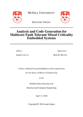
4.1.3 Four Mode QoS Results for Single Core
We defined QoS to be the percentage of LO criticality tasks not dropped in any given mode.
The QoS for the LO mode is always 1. Random task sets were generated according to the
UUnifast algorithm [39] such that LO mode utilization is approximately 80% on all cores. The
ratio C(HI)/C(LO) is determined randomly from the range [1, 2] and periods were chosen at
random from the set 10, 20, 40, 50, 100, 200, 400, 500, 1000. For each test, the average of 1000
systems is presented.
FIGURE 4.3: Modes OV and TF achieve better QoS than HI for all utilizations
(F not bounded).
Figure 4.3 shows the QoS of OV and TF modes is improved over the HI mode for all
utilizations in systems of 20 tasks (10 HI and 10 LO). LO task QoS is better in the OV and
TF modes than in the HI mode. On average, the OV and TF modes outperform the HI mode
by 42.9% and 20.2% respectively. The improvement increases with the utilization, especially
for the OV mode which could be significant in systems where transient faults are less frequent
52. Chapter 4. Mapping and Scheduling 40
FIGURE 4.4: Average improvement over all system utilizations for OV and TF
modes compared to HI mode.
than execution time overruns. Figure 4.4 shows the average improvement of QoS across all
utilizations for the TF and OV mode compared to the HI mode.
FIGURE 4.5: Modes OV and TF achieve better QoS than HI for different per-
centages of HI tasks (F not bounded).
Figure 4.5 shows a similar picture, this time holding utilization constant at 80% while ex-
ploring the percentage of HI tasks. The QoS of the HI and TF modes degrade quickly as the
percentage of HI tasks increases because none of these tasks can be dropped and the penalty
for re-execution becomes very severe.
Figure 4.6 shows how the F parameter improves QoS for the TF mode (F = ∞ is the de-
fault). QoS improves by about 15% compared to the default when only two errors are assumed
53. Chapter 4. Mapping and Scheduling 41
FIGURE 4.6: Performance of TF mode for different F
to occur close enough in time to affect the same mode change.
4.2 Extending Response Time Analysis to ODR
We will extend the analysis on lockstep (LS) to support three types of ODR. The four scenarios
(including lockstep) are shown in Figure 4.7. In (a), LS execution occurs when a node has
internal mechanisms for detecting but not correcting errors. An error simply results in a re-
execution on that node, as previously discussed. In (b), dual modular redundancy (DMR)
replicates a thread on two cores that cannot detect errors by themselves. The task must be
re-executed if the executions do not match according to some external comparison or voting
mechanism. In (c), triple modular redundancy (TMR) replicates a thread on three cores that
cannot detect errors. If an error occurs, the majority answer is taken from the three replicas and
no re-execution is required (the system assumes only one replica may fail at a time). Finally, in
(d), passive replication is similar to TMR but the final replica does not execute if the first two
copies return the same result.
Each technique is expressed in the new analysis by three parameters: a task set transforma-
tion, mapping constraints, and a re-execution profile denoted by N. The task set transformation
represents each replica explicitly in the task set. Consider the example task set in Table 4.2.
Lockstep does not introduce any replicas to the system and does not require any transformation
54. Chapter 4. Mapping and Scheduling 42
FIGURE 4.7: The 4 fault tolerance mechanisms supported by the proposed
MCFTS analysis
TABLE 4.2: Task set transformations
(A) Example task set
C(LO) C(HI) T=D L
τ1 5 10 25 HI
τ2 5 - 20 LO
(B) DMR transformation
C(LO) C(HI) T=D L
τ1 5 10 25 HI
τ1.1 5 10 25 HI
τ2 5 - 20 LO
π1 = π1.1
(C) TMR transformation
C(LO) C(HI) T=D L
τ1 5 10 25 HI
τ1.1 5 10 25 HI
τ1.2 5 10 25 HI
τ2 5 - 20 LO
π1 = π1.1 = π1.2
(D) PR replication
C(LO) C(HI) T=D L
τ1 5 10 25 HI
τ1.1 5 10 25 HI
τ1.2 5 10 25 HI
τ2 5 - 20 LO
π1 = π1.1
of the task set. DMR requires one replica to be added to the task set while TMR and PR require
two replicas to be added.
Constraints must be added to the problem for the processors πi assigned to τi in order to
properly reflect the semantics of the different techniques. The constraints shown in the table
ensure that the replicas are not assigned to the same core. These constraints will be useful in
the mapping stage.
The re-execution variable ni has been generalized into the vector:
Ni =< ni(LO), ni(OV ), ni(TF), ni(HI) > (4.8)
55. Chapter 4. Mapping and Scheduling 43
TABLE 4.3: Re-execution profiles for the fault tolerance mechanisms
Technique Profile (N)
LS < 1, 2, 1, 2 >
DMR < 1, 2, 1, 2 >
TMR < 1, 1, 1, 1 >
PR < 1, 1, 1, 1 > and < 0, 1, 0, 1 >
The N for each mode is shown in Table 4.3 and the updated equation for the OV mode response
time are given by the following equations:
R
(OV )
i =
Ci(Li) +
j∈hpC(OV,i)
R
(OV )
i
Tj
· Cj(Lj)
+
k∈hp(i)−hpC(OV,i)
R
(LO)
i
Tk
· Ck(LO), ni(OV ) > 0
0, ni(OV ) = 0
(4.9)
We note that all techniques have n(LO) and n(OV ) values of either 0 or 1. When n = 0, the
task is not executing and the response time is simply 0. The same is true for LO mode.
For example, TMR has N =< 1, 1, 1, 1 >. This means that in all modes, any task using
TMR will have n = 1 which in effect signals that no re-executions are required. For PR, one
replica executes one time in all modes and the other only executes in the case of a fault (hence
only executes once in TF or HI modes).
4.3 Design Space Exploration
4.3.1 Genetic Algorithm
Genetic algorithm is an unsupervised exploration technique that attempts to find optimal an-
swers in large problem spaces [40]. Genetic algorithms operate on chromosomes which are
essentially a vector representation of the problem space. An initial population of chromosomes
are rated using an objective or fitness function which determines the quality of each result. If a
56. Chapter 4. Mapping and Scheduling 44
Generate new
Population
Input
Population
Objective
Function
Criteria
Met?
Best
Individuals
Y
Selection
N
Result
Recombine
Mutate
FIGURE 4.8: The basic structure of a genetic algorithm [40].
sufficient answer has been found then the algorithm may quit. Otherwise, a new population is
generated using selection, recombination and mutation.
There are many variations on each of these operations. Selection could be as simple as pass-
ing on the top x chromosomes and then randomly generating the remainder of the population
after each generation. Another alternative is tournament selection, where pairs of chromo-
somes are selected randomly from the population and the higher of the two is passed on to the
next generation. Recombination is typically done using the crossover operator which chops two
chromosomes at some gene location (element index) and swaps the ends. Finally mutation ran-
domly modifies a randomly selected gene in a randomly selected chromosome. There are many
probabilistic parameters that require calibration for each operator as well as the population size
and number of generations.
There is not a generally well defined methodology for selecting these parameters. These
experiments will evolve a population of size 100 over 30 generations. 80% of chromosomes
are selected from the previous generation using tournament selection. The tournament selection
itself passes on the best chromosomes with a probability of 80%. The crossover rate is 40%
and the mutation rate is 50%. The mutation and crossover rates are fairly high however only
57. Chapter 4. Mapping and Scheduling 45
the fittest chromosome is required (rather than a population of highly fit chromosomes). We
are not concerned with building a fit population therefore higher mutation rates ensures that
each generation changes with respect to its predecessor and many different chromosomes (i.e. a
larger portion of the design space) are tested. Furthermore, we allow the algorithm to optionally
quit early if several generations pass without finding a new answer. Therefore, increasing the
size of the population ensures a certain minimum number of chromosomes have been tested.
4.3.2 Two Stage GA
The mapping and scheduling algorithm follows the procedure used in [41] and [42]. Two
stages of genetic algorithms (GA), implemented using JGAP [43], are used to explore both the
techniques used to harden each task and the core assignment for each task and its replicas. The
basic flow is shown in Figure 4.9. The Reliability Aware (RA) stage is responsible for mapping
a fault tolerance mechanism to each task. The RA stage then generates a chromosome structure
for the Mapping and Scheduling (MS) stage. The MS stage attempts to find an allocation for
each task onto a core that maximizes the average QoS across all modes in the system using the
response time analysis from Section 4.1. It is necessary to define the problem in terms of a
chromosome for each stage.
FIGURE 4.9: Overview of DSE workflow using nested genetic algorithm
searches
The chromosome in the RA stage has one integer gene for each task representing a fault
tolerance mechanism. For instance, consider a task set with two HI tasks τ1, τ2 being mapped
onto a platform that supports LS, DMR and TMR - the chromosome would consist of two genes
each limited to integers in the range [0, 2].
58. Chapter 4. Mapping and Scheduling 46
TABLE 4.4: Rules for generating unique MS configurations from an integer x for
n cores
Technique Configurations Conversion Rule
none n (x)
LS n (x)
DMR n(n − 1) ( x
n−1
, x mod (n − 1))
TMR n(n − 1)(n − 2) ( x
(n−1)(n−2)
, x mod ((n−1)(n−2))
n−2
, x mod (n − 2))
PR n2
(n − 1) ( x
n(n−1)
, x mod (n(n−1))
n−1
, x mod (n − 1))
The RA fitness function (FF) must determine the fitness (QoS) for each configuration of
fault tolerance mechanisms. The FF creates a new task set using the transformations in Ta-
ble 4.2 as well as the necessary constraints. The FF then creates a chromosome template for
the MS stage based on the transformed task set. Given the number of processors that a task
can be mapped to, n, it is possible to determine for each FTM a mapping rule that generates a
unique configuration from an integer. It is important that the task and replicas are represented
by a single gene or else most chromosomes will result in illegal configurations after mutation
and crossover. Table 4.4 shows the number of configurations for each type of FTM and how
to derive a unique allocation as a function of the number of candidate cores (n) from a random
integer x < n. The conversion rule provides an index into an ordered list of the cores. A core
is removed from the list once it is allocated.
For example, consider a task and two replicas using TMR in a sytem with 5 processing
cores. All three tasks must go on different cores. The number of configurations is 5 · 4 · 3 = 60.
The GA will generate a random integer in the range [0, 59] representing a unique mapping of the
three tasks onto the system, say 47. The number 47 is converted using the TMR rule to (47/(4·
3), (47 mod (4 · 3))/3, 47 mod 3) = (3, 3, 1). Suppose the core list is {π1, π2, π3, π4, π5}. The
first copy is allocated to π3 and π3 is then removed from the list. The next copy is assigned to
π4 (now at index 3) and the third copy is assigned to π1.
A unique MS stage is instantiated for each chromosome in the RA stage population. The
MS stage generates a population based on the chromosome built by the RAFF. The MSFF
builds each chromosome into a schedule and passes it along to the schedulability analysis. If
the system is schedulable then the chromosome is assigned a fitness value equal to the average
59. Chapter 4. Mapping and Scheduling 47
QoS across all four modes (defined as percentage of LO tasks that have not been dropped). If
the analysis fails then the chromosome is assigned a fitness value of 0.
4.3.3 Performance Optimization
The performance overhead of nesting one lengthy search inside another is potentially thousands
of times more expensive depending on the population size and number of iterations. However,
the overall runtime can be shortened with sufficient parallel computing resources. The JGAP
library was modified to allow the RA stage to request a new thread from a pool whenever
calling the RA fitness function, allowing for the parallel execution of the MS stage for each
chromosome in the RA population. Using 20 threads on a 30 core system resulted in an average
speedup of approximately 15x and makes this a much more practical implementation given
sufficient computing resources. We furthermore implement early exiting if a solution is found
with perfect QoS or the best QoS has not been improved in four generations.
4.3.4 Results
Three platforms were tested to verify the mapping: one system (ODR) with four cores using
only DMR, the second (LS) with two lockstep cores, and the third (FP) using one lockstep
core and two processing cores using DMR. The same task generation algorithm was used as in
Section 4.1.3. The systems were tested with 100 task sets with between 20 and 40 tasks, half of
which were HI, an average utilization of 80%, and a maximum WCET factor (C(HI)/C(LO))
of 3. Note that for the ODR and LS systems, the RA stage could be skipped for efficiency
purposes as there is only one available mechanism.
Any system that is schedulable for one system should be schedulable for all three. They
should only differ (possibly) in the QoS of each mode. Furthermore, we expect the QoS of the
ODR and FP systems to be higher than that of the LS.
Figure 4.10 compares the QoS in the HI mode for the different hardware configurations as
system utilization varies. 20 tasks were scheduled, with half on average HI. The QoS for MIX
and ODR are on average 20% better than for LS and 30% in the worst case. Figure 4.11 shows
60. Chapter 4. Mapping and Scheduling 48
similar results with the percentage of HI tasks varied while utilization is held constant at 0.7.
In both cases we observe that ODR provides better resource utilization on average as resource
utilization increases. The results do not take into account possible voting overheads or recovery
delays that might further differentiate between the MIX and ODR platforms.
FIGURE 4.10: ODR provides better QoS in multicore systems as utilization in-
creases in the HI mode.
FIGURE 4.11: ODR provides better QoS in multicore systems as the percentage
of HI tasks increases.
Figures 4.12 and 4.13 compare the QoS and schedulability, respectively, for two ODR plat-
forms with different fault tolerance mechanisms available. The first system is only capable of
DMR (DMR) while the second system is capable of all three varieties of ODR studied in this
61. Chapter 4. Mapping and Scheduling 49
paper (DMR+TMR+PR). We observe that in general more varieties of ODR improves both
schedulability and QoS. The different techniques provide greater flexibility in how to distribute
the workload across the cores.
FIGURE 4.12: Combining several ODR techniques improves QoS
FIGURE 4.13: Combining several ODR techniques improves schedulability
62. Chapter 5
Code Generation
The code generation framework is designed to automate the porting of Simulink generated con-
trol algorithms to the architecture presented in Figure 2.3. The structure of the application be-
ing ported follows the assumptions made in the schedulability analysis presented in Chapter 4,
mainly that tasks are independent and periodic, and that an optimistic and pessimistic WCET
have been specified. The hardware and generated code support both DMR with re-execution
and TMR for error correction, as well as execution time monitoring. Only a simplified two
mode model has been implemented at this time.
Error detection is implemented using fingerprinting hardware where checksums based on
the execution stream are compared to ensure correct operation. Local scratchpads are used in
combination with memory protection and memory virtualization to ensure that data is quaran-
tined within the sphere of replication until the results have been verified. A trusted monitor
is responsible for data management and replication across the entire system. Code generation
requires well defined protocols for the monitor and processing core that can be translated into
C templates. Several issues must be addressed for correct operation: deterministic thread ex-
ecution, fault containment, execution time monitoring, data transfer, and task re-execution in
case of fault.
Figure 5.1 shows the system level control flow for a correct execution of a DMR replicated
task. The monitor core (FTC), the processing core, the fingerprint (FP) unit, and the comparator
are the main components in the system that implement ODR. First the monitor configures the
comparator. Then the monitor prepares and sends the data and stack to the scratchpads (SPM)
50
63. Chapter 5. Code Generation 51
of both processing cores. The monitor then notifies the cores to begin execution of the critical
task. Each core notifies its FP unit that a critical task is beginning. The FP units then notify the
comparator. The FP units send the checksum to the comparator when a task is complete. When
all checksums are received the comparator notifies the monitor of the result. If the execution is
correct the monitor then copies back one of the correct scratchpad contents.
FIGURE 5.1: The main sequence of operations in correct execution of a dis-
tributed task on the platform
Section 5.1.1 provides an overview of the memory architecture. Section 5.1.2 then provides
details on the monitor behaviour corresponding to the flow in Figure 5.1 as well as for the case
when a transient error is detected. Section 5.1.3 finishes with the implementation details for
the processing cores. Section 5.2 presents the code generation procedure. Section 5.3 presents
several examples of generated applications.
5.1 Software Implementation
5.1.1 Memory Architecture
The memory architecture in Figure 5.2 contains several specialized modules and regions of
access to enforce fault containment and deterministic execution in redundant threads. Each
core has an MPU to enforce memory protection and uTLB for virtual memory management.
As previously mentioned, each core executes on copies of data in the SPM while the original
64. Chapter 5. Code Generation 52
copy remains unaltered in main memory. The MPU is used to ensure that the cores do not access
the original copy of the data. In a future implementation, a centralized MPU managed strictly
by the monitor would be more dependable. The current MPU is contained in the closed-source
Nios code and cannot be modified or extended.
FIGURE 5.2: Memory partition of local and global data space.
The shared memory is a region of fast on-chip memory used for inter-core communication.
The monitor must pass some information to the processing cores at each task execution such
as fingerprint ID (see [6] for details) and the scratchpad pages allocated to the task (discussed
below). All data in shared memory is written by only one core to simplify concurrent data
accesses.
The physical address space is partitioned in order to support a simple virtual memory
scheme. The monitor is responsible for copying critical data into the scratchpads and back
to main memory using a DMA module connected to each scratchpad.
Virtual Memory Management
Fingerprinting requires the address and data to match for all store instructions which in turn
requires that the stack pointer be identical on both cores throughout the execution of the task.
Deterministic behaviour is guaranteed by fingerprinting the virtual address and ensuring that
65. Chapter 5. Code Generation 53
both cores use the same virtual address. The uTLB translates the virtual address into the physi-
cal address and is programmed by each core according to runtime information provided by the
monitor.
The uTLB translates addresses in the typical fashion with a table of the upper bits of phys-
ical and virtual addresses. The memory space is separated into pages aligned to the first bit
that may be translated. The uTLB setup requires that virtual memory management be handled
entirely in software as there are no complex data structures such as page tables or MMU to
consult them in the background.
Several assumptions are enforced by the virtual memory protocol in order to simplify the
implementation. Every task has a stack and global data that each consume one 4kB page. The
uTLB page size is 4kB and each line is statically assigned to translation of the data or stack of
a single task. The scratchpad is divided evenly into 4kB pages which are dynamically allocated
to a task, thus requiring dynamic updating of the translation table values.
The virtual memory protocol divides each scratchpad into bins according to the page size
used by the uTLB. A 16kB scratchpad, for example, contains four bins of 4kB pages. The linker
script for each core is updated to reserve one page in main memory for the global data (currently
one 4kB page is reserved for all global data of fingerprinted tasks rather than on a per-task
basis) and one for the stack of each task. The stack size of each task is known statically using
profiling information and adding an offset to account for the overhead of context switching and
interrupt handling. The virtual address for each stack is assigned statically at design time. The
physical address may changes at runtime as the scratchpad location is dynamically assigned
and may change as required to support preemption (Section 14). The virtual addresses of all
stacks point to an unused section of the address space to ensure that no data is corrupted if
translation malfunctions or is accidentally turned off.
Each core is initially assigned 200kB of main memory. The stack bins are removed from
the end of the main memory allocation by modifying the linker script. Listing 5.1 shows the
main memory region of a core has been shortened by 8kB (from 204768 to 196576 on line 5)
and two 4kB regions called stack_bin_x have been added. Listing 5.2 shows a condensed