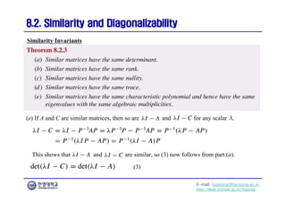
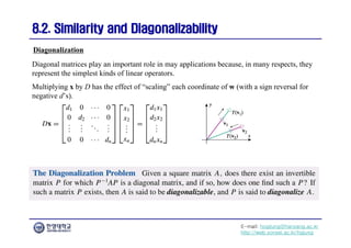
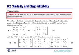
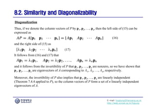
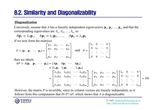
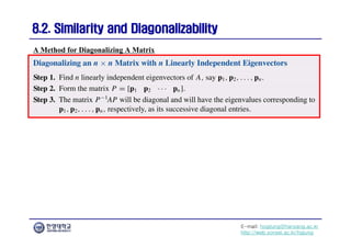
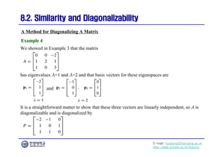
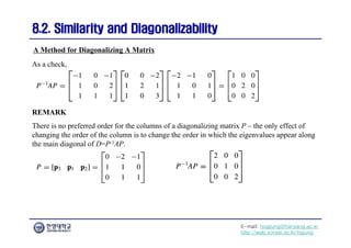
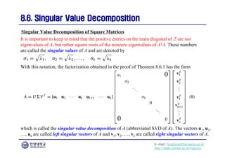
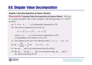
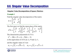
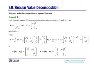
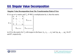
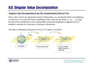
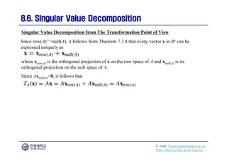
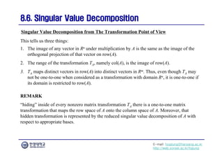
The document focuses on the matrix representations of linear transformations, particularly the construction of standard matrices and their geometric implications. It discusses different bases for linear operators and how changing bases impacts the representation of these operators. Additionally, it explores the concept of similarity and diagonalizability of matrices, highlighting properties that are invariant under similarity transformations.

![E-mail: hogijung@hanyang.ac.kr
http://web.yonsei.ac.kr/hgjung
8.1. Matrix Representations of Linear Transformations
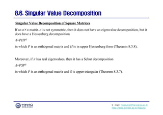
8.1. Matrix Representations of Linear Transformations
We know that every linear transformation T: RnRm has an associated standard matrix
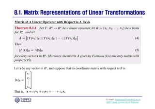
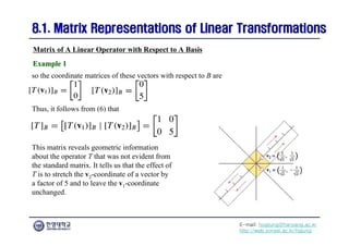
Matrix of A Linear Operator with Respect to A Basis
with the property that
for every vector x in Rn. For the moment we will focus on the case where T is a linear operator
on Rn, so the standard matrix [T] is a square matrix of size n×n.
Sometimes the form of the standard matrix fully reveals the geometric properties of a linear
operator and sometimes it does not.
Our primary goal in this section is to develop a way of using bases other than the standard
basis to create matrices that describe the geometric behavior of a linear transformation better
than the standard matrix.](https://image.slidesharecdn.com/diagonalization-240722231727-0a90b72e/85/Some-lecture-notes-on-diagonalization-of-matrices-2-320.jpg)
![E-mail: hogijung@hanyang.ac.kr
http://web.yonsei.ac.kr/hgjung
8.1. Matrix Representations of Linear Transformations
8.1. Matrix Representations of Linear Transformations
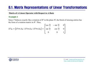
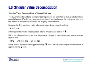
Matrix of A Linear Operator with Respect to A Basis
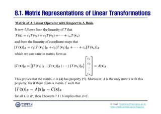
Suppose that
is a linear operator on Rn and B is a basis for Rn. In the course of mapping x into T(x) this
operator creates a companion operator
that maps the coordinate matrix [x]B into the coordinate matrix [T(x)]B.
There must be a matrix A such that](https://image.slidesharecdn.com/diagonalization-240722231727-0a90b72e/85/Some-lecture-notes-on-diagonalization-of-matrices-3-320.jpg)
![E-mail: hogijung@hanyang.ac.kr
http://web.yonsei.ac.kr/hgjung
8.1. Matrix Representations of Linear Transformations
8.1. Matrix Representations of Linear Transformations
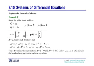
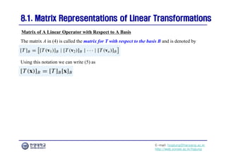
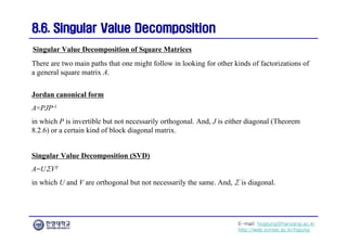
The rotation leaves the vector v3 fixed, so
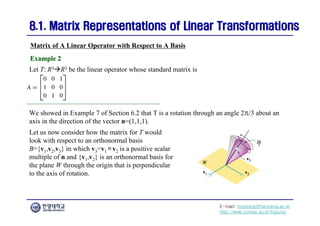
Matrix of A Linear Operator with Respect to A Basis
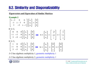
Example 2
Example 2
and hence
Also, T(v1) and T(v2) are linear combinations of v1 and v2, since these vectors lie in W. This
implies that the third coordinate of both [T(v1)]B and [T(v2)]B must be zero, and the matrix for
T with respect to the basis B must be of the form](https://image.slidesharecdn.com/diagonalization-240722231727-0a90b72e/85/Some-lecture-notes-on-diagonalization-of-matrices-10-320.jpg)
![E-mail: hogijung@hanyang.ac.kr
http://web.yonsei.ac.kr/hgjung
8.1. Matrix Representations of Linear Transformations
8.1. Matrix Representations of Linear Transformations
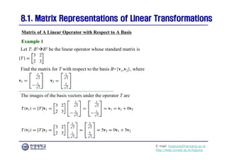
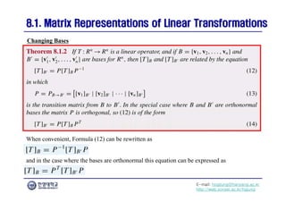
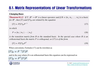
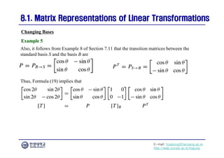
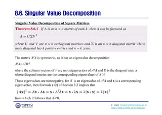
Suppose that T: RnRn is a linear operator and that B={v1,v2,…,vn} and B’={v’1,v’2,…,v’n}
are bases for Rn. Also, let P=PBB’ be the transition matrix from B to B’ (so P-1=PB’B is the
transition matrix from B’ to B).
Changing Bases
The diagram shows two different paths from [x]B’ to [T(x)]B’:
(11)
(10)
1.
2.
Thus, (10) and (11) together imply that
Since this holds for all x in Rn, it follows from Theorem 7.11.6 that](https://image.slidesharecdn.com/diagonalization-240722231727-0a90b72e/85/Some-lecture-notes-on-diagonalization-of-matrices-12-320.jpg)
![E-mail: hogijung@hanyang.ac.kr
http://web.yonsei.ac.kr/hgjung
8.1. Matrix Representations of Linear Transformations
8.1. Matrix Representations of Linear Transformations
Since many linear operators are defined by their standard matrices, it is important to consider
the special case of Theorem 8.1.2 in which B’=S is the standard basis for Rn.
In this case [T]B’=[T]S=[T], and the transition matrix P from B to B’ has the simplified form
Changing Bases](https://image.slidesharecdn.com/diagonalization-240722231727-0a90b72e/85/Some-lecture-notes-on-diagonalization-of-matrices-14-320.jpg)
![E-mail: hogijung@hanyang.ac.kr
http://web.yonsei.ac.kr/hgjung
8.1. Matrix Representations of Linear Transformations
8.1. Matrix Representations of Linear Transformations
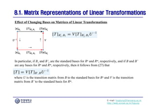
Formula (17) [or (19) in the orthogonal case] tells us that the process of changing from the
standard basis for Rn to a basis B produces a factorization of the standard matrix for T as
Changing Bases
in which P is the transition matrix from the basis B to the standard basis S. To understand the
geometric significance of this factorization, let us use it to compute T(x) by writing
Reading from right to left, this equation tells us that T(x) can be obtained by first mapping the
standard coordinates of x to B-coordinates using the matrix P-1, then performing the operation
on the B-coordinates using the matrix [T]B, and then using the matrix P to map the resulting
vector back to standard coordinates.](https://image.slidesharecdn.com/diagonalization-240722231727-0a90b72e/85/Some-lecture-notes-on-diagonalization-of-matrices-16-320.jpg)
![E-mail: hogijung@hanyang.ac.kr
http://web.yonsei.ac.kr/hgjung
8.1. Matrix Representations of Linear Transformations
8.1. Matrix Representations of Linear Transformations
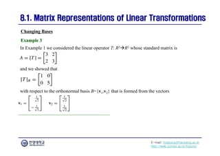
In this case the transition matrix from B to S is
Changing Bases
Example 3
Example 3
so it follows from (17) that [T] can be factored as](https://image.slidesharecdn.com/diagonalization-240722231727-0a90b72e/85/Some-lecture-notes-on-diagonalization-of-matrices-18-320.jpg)
![E-mail: hogijung@hanyang.ac.kr
http://web.yonsei.ac.kr/hgjung
8.1. Matrix Representations of Linear Transformations
8.1. Matrix Representations of Linear Transformations
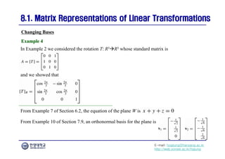
Since v3=v1×v2,
Changing Bases
Example 4
Example 4
The transition matrix from B={v1,v2,v3} to the standard basis is
Since this matrix is orthogonal, it follows from (19) that [T] can be factored as](https://image.slidesharecdn.com/diagonalization-240722231727-0a90b72e/85/Some-lecture-notes-on-diagonalization-of-matrices-20-320.jpg)
![E-mail: hogijung@hanyang.ac.kr
http://web.yonsei.ac.kr/hgjung
8.1. Matrix Representations of Linear Transformations
8.1. Matrix Representations of Linear Transformations
Recall that every linear transformation T: RnRm has an associated m×n standard matrix
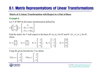
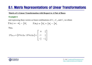
Matrix of A Linear Transformation with Respect to A Pair of Bases
with the property that
If B and B’ are bases for Rn and Rm, respectively, then the transformation
creates an associated transformation
that maps the coordinate matrix [x]B into the coordinate matrix [T(x)]B’. As in the operator
case, this associated transformation is linear and hence must be a matrix transformation; that is,
there must be a matrix A such that](https://image.slidesharecdn.com/diagonalization-240722231727-0a90b72e/85/Some-lecture-notes-on-diagonalization-of-matrices-23-320.jpg)
![E-mail: hogijung@hanyang.ac.kr
http://web.yonsei.ac.kr/hgjung
8.1. Matrix Representations of Linear Transformations
8.1. Matrix Representations of Linear Transformations
The matrix A in (23) is called the matrix for T with respect to the bases B and B’ and is
denoted by the symbol [T]B’,B.
Matrix of A Linear Transformation with Respect to A Pair of Bases](https://image.slidesharecdn.com/diagonalization-240722231727-0a90b72e/85/Some-lecture-notes-on-diagonalization-of-matrices-24-320.jpg)
![E-mail: hogijung@hanyang.ac.kr
http://web.yonsei.ac.kr/hgjung
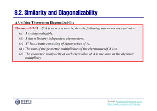
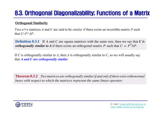
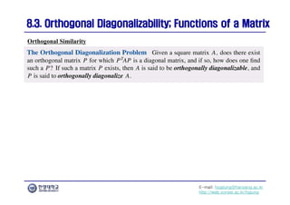
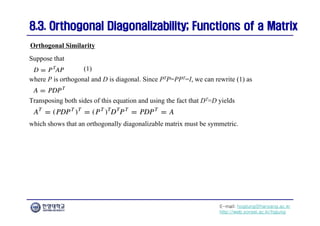
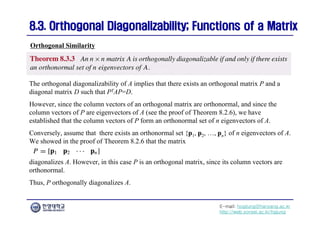
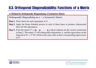
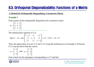
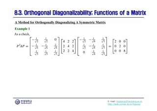
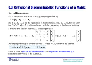
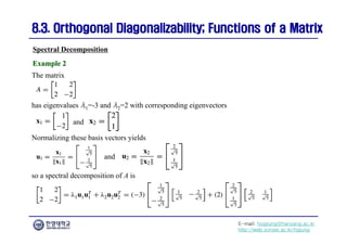
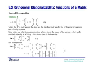
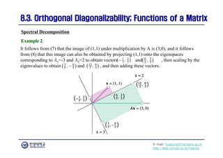
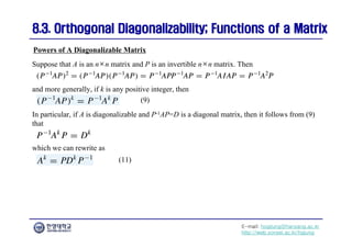
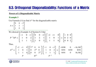
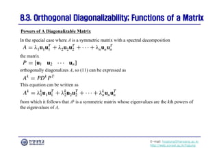
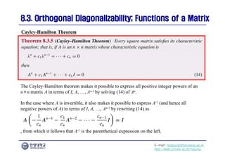
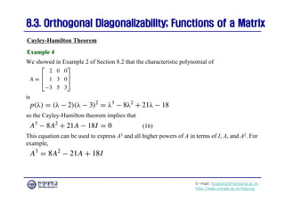
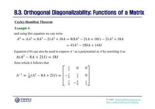
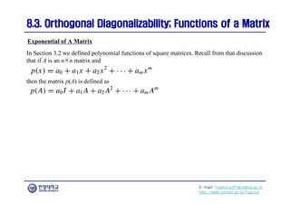
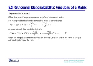
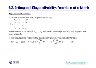
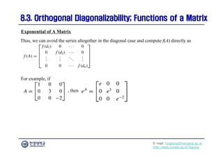
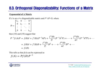
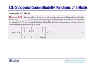
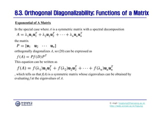
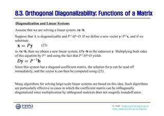
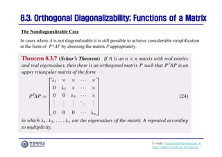
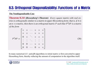
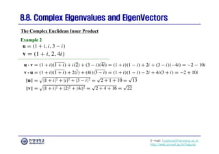
8.3. Orthogonal Diagonalizability; Functions of a Matrix
8.3. Orthogonal Diagonalizability; Functions of a Matrix
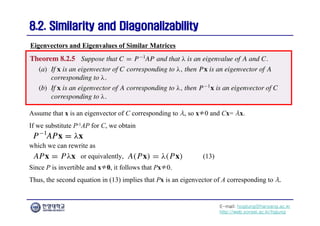
(b) Let v1 and v2 be eigenvectors corresponding to distinct eigenvalues λ1 and λ2, respectively.
The proof that v1·v2=0 will be facilitated by using Formula (26) of Section 3.1 to write
λ1 (v1·v2)=(λ1v1)·v2 as the matrix product (λ1v1)Tv2. The rest of the proof now consists of
manipulating this expression in the right way:
Orthogonal Similarity
[v1 is an eigenvector corresponding to λ1]
[symmetry of A]
[v2 is an eigenvector corresponding to λ2]
[Formula (26) of Section 3.1]
This implies that (λ1- λ2)(v1·v2)=0, so v1·v2=0 as a result of the fact that λ1≠λ2.](https://image.slidesharecdn.com/diagonalization-240722231727-0a90b72e/85/Some-lecture-notes-on-diagonalization-of-matrices-57-320.jpg)

![E-mail: hogijung@hanyang.ac.kr
http://web.yonsei.ac.kr/hgjung
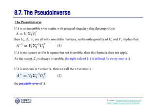
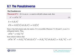
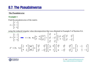
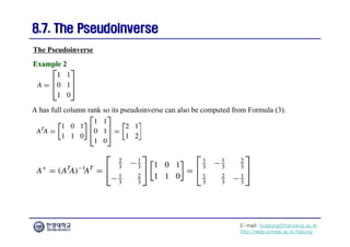
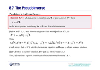
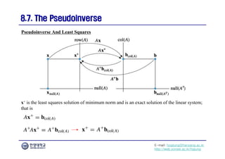
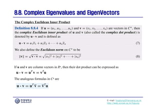
8.7. The Pseudoinverse
8.7. The Pseudoinverse
(b) Multiplying A+ on the right by U1 yields
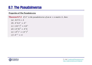
Properties of The Pseudoinverse
The result now follows by comparing corresponding column vectors on the two sides of this
equation.
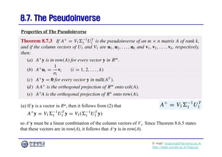
(c) If y is a vector in null(AT), then y is orthogonal to each vector in col(A), and, in particular,
it is orthogonal to each column vector of U1=[u1, u2, …, uk].
This implies that U1
Ty=0, and hence that](https://image.slidesharecdn.com/diagonalization-240722231727-0a90b72e/85/Some-lecture-notes-on-diagonalization-of-matrices-156-320.jpg)
![E-mail: hogijung@hanyang.ac.kr
http://web.yonsei.ac.kr/hgjung
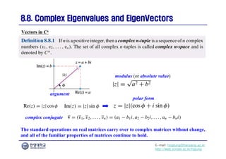
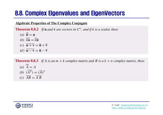
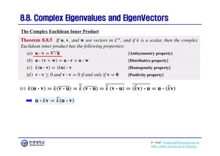
8.8. Complex Eigenvalues and
8.8. Complex Eigenvalues and EigenVectors
EigenVectors
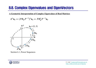
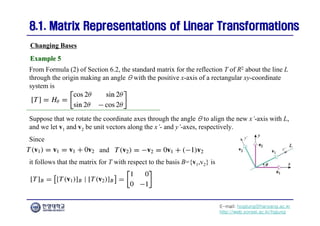
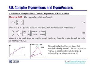
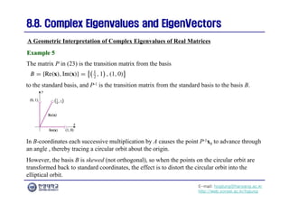
A Geometric Interpretation of Complex Eigenvalues of Real Matrices
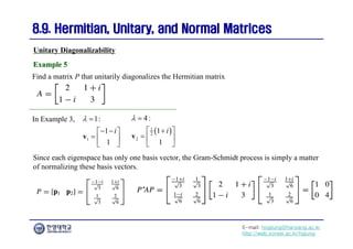
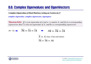
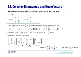
Example 5
Example 5
3 3
1 4
1
2 4 5 5
2
3 3 1
11 4
2
5 10 5 5
0 1
1 1
1
1
1 1
1 0
3
4
1
5 5
2
3 1
4
2
5 5
1
1
1 0
1 1
2 2
1
1 0 1
5
4
1
2
[x0 is mapped to B-coordinates]
[The point (1,1/2) is rotated through the angle φ]
[The point (1/2,1) is mapped to standard coordinates]](https://image.slidesharecdn.com/diagonalization-240722231727-0a90b72e/85/Some-lecture-notes-on-diagonalization-of-matrices-176-320.jpg)