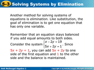
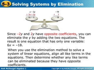
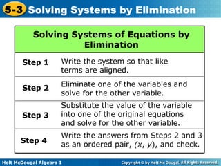
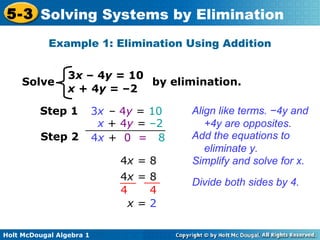
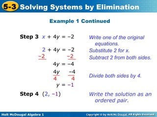
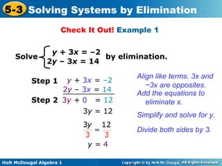
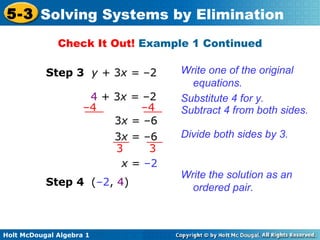
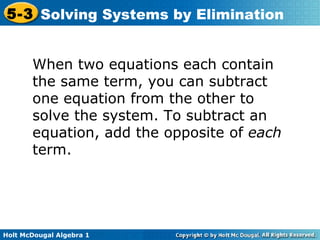
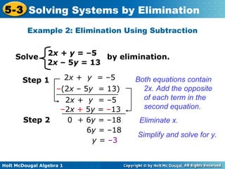
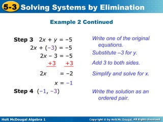
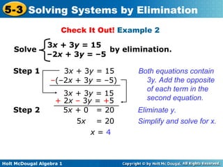
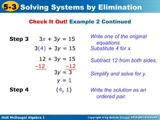
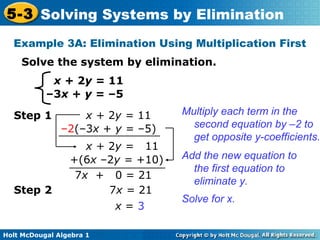
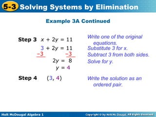
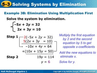
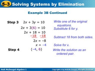
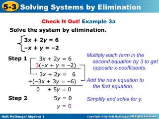
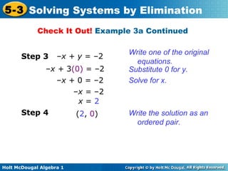
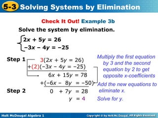
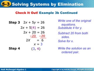
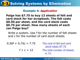
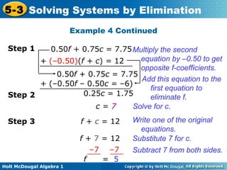
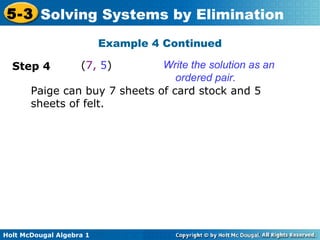
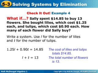
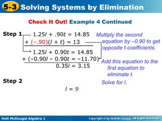
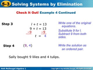
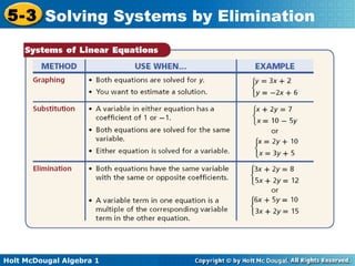
Learning Objective(s)
· Solve a system of equations when no multiplication is necessary to eliminate a variable.
· Solve a system of equations when multiplication is necessary to eliminate a variable.
· Recognize systems that have no solution or an infinite number of solutions.
· Solve application problems using the elimination method.
I have added to the original presentation in response to one of the comments.... the result of 'x' is correct on slide 7, take a look at the new version of this ppt to clear up any confusion about why...
This document discusses using x-intercepts and y-intercepts to graph linear functions. It provides 4 examples of finding the x-intercept and y-intercept of linear equations by setting either x or y equal to 0 and solving for the other variable. The x-intercept is the x-coordinate where the line crosses the x-axis (when y=0) and the y-intercept is the y-coordinate where the line crosses the y-axis (when x=0).
1) This document discusses double-angle and half-angle formulas for trigonometric functions like sine, cosine, and tangent.
2) It derives formulas that relate trig functions of double and half angles to trig functions of the original angle, such as sin(2x) = 2sin(x)cos(x) and sin(x/2) = ±√(1-cos(x))/2.
3) Examples are provided to demonstrate applying these formulas to simplify trigonometric expressions and derive new identities.
The document discusses direct and inverse variation. It provides examples of questions determining if a relationship demonstrates direct or inverse variation. It also shows how to write the equation for a direct or inverse variation relationship given data points. Direct variation follows the equation y=kx, where k is the constant rate of change. Inverse variation follows y=k/x. The document provides step-by-step workings for multiple examples of identifying and modeling direct and inverse variation relationships from sets of data points.
Quadratic equations are equations of the form ax^2 + bx + c = 0, where a ≠ 0. They are called quadratic because the highest exponent is 2. The standard form is ax^2 + bx + c = 0. Quadratic equations can be solved using the quadratic formula. They are useful for modeling real-world problems involving time, velocity, distance, height, area, length, speed, cost, and benefits. An example is designing a new sports bike and using a quadratic equation to determine how many to produce for maximum profit.
1) A composite function is formed by combining two functions, where one function is substituted into the other.
2) Notations like fg(x) indicate that function g(x) is substituted into function f(x).
3) Composite functions are non-commutative, meaning the order of the functions matters - fg(x) may not equal gf(x).
- The order of a root of a polynomial is the number of times the root repeats.
- The polynomial x5 + 2x4 + x3 has two roots, x = 0 with order 3 and x = -1 with order 2.
- In general, polynomials of the form k(x - c1)m(x - c2)m...(x - cn)m have roots x = c1 with order m1, x = c2 with order m2, and so on.
The document discusses higher order derivatives. It defines the nth derivative of a function f(x) as f(n)(x). The first example finds the first five derivatives of f(x)=2x^4 - x^3 - 2. The second example finds the first three derivatives of f(x)=-x^2/3. The third example finds the first four derivatives of f(x)=ln(x) and discusses how derivatives of rational functions become more complicated with higher orders. It also provides examples of finding derivatives of other functions like sin(x).
1) An inverse function f^-1 interchanges the x and y values of the original function f.
2) For a function to have an inverse, it must be one-to-one, meaning each x maps to a single y and vice versa.
3) To find the inverse of a function algebraically, interchange x and y and solve for y. The graph of an inverse is the reflection of the original graph across the line y=x.
This document discusses how to graph polynomial functions and find local extrema. It provides instructions on making a table of values, plotting points, connecting them with a smooth curve, and checking end behavior based on the degree and leading coefficient. Extrema are defined as local maxima or minima, where the graph changes from increasing to decreasing. Examples are given to demonstrate graphing polynomials and finding turning points that indicate local extrema.
The document discusses the fundamental counting principle, which states that if one task can be completed in n ways and a second task can be completed in m ways, the total number of ways both tasks can be completed is n x m. It provides examples of applying this principle, such as a party with 3 juice options and 4 dessert options resulting in 3 x 4 = 12 possible juice-dessert pairs. The document also explains that outfits have 8 blouse options, 4 skirt/pants options, and 3 shoe options, so there are 8 x 4 x 3 = 96 possible outfits according to the fundamental counting principle.
This document provides a lesson on writing and graphing linear equations in slope-intercept form. It begins with examples of finding the slope and y-intercept of lines and writing the equation in the form y = mx + b. Then it shows how to graph lines from their equations in slope-intercept form. Applications include writing cost functions and finding values. A quiz reviews writing equations from slopes and points and graphing lines from their equations.
The document discusses piecewise functions, which are functions defined by multiple rules over different parts of the domain. It provides examples of piecewise functions, including how to graph them by applying each rule over the appropriate portion of the domain. It also discusses evaluating piecewise functions at given values, writing piecewise functions based on graphs, and analyzing properties like extrema. Piecewise functions allow modeling of real-world situations using multiple equations each corresponding to a part of the input range.
This document discusses finding the sum and product of the roots of quadratic equations. It provides the formulas for calculating the sum and product of roots without explicitly solving for the individual roots. The sum of the roots is equal to -b/a, and the product of the roots is equal to c/a, where a, b, and c are the coefficients of the quadratic equation in the standard form ax^2 + bx + c = 0. Several examples are worked out applying these formulas. The document also contains exercises asking the reader to find the sum and product of roots for additional quadratic equations using the given coefficients a, b, and c.
The document defines proper and improper integrals, and discusses different types of improper integrals based on whether the limits are infinite or the function is unbounded. It provides tests to determine if improper integrals converge or diverge, including the T1 test involving exponential functions, the T2 test involving power functions, and comparison tests. Examples are worked through applying these tests to determine if various improper integrals converge or diverge. The key information is on defining improper integrals and tests to analyze their convergence.
3 αρχεία στη Γ λυκείου! Ποδαρικό με το δεξί για το lisariΜάκης Χατζόπουλος
Επιμέλεια: Τριαντάφυλλος Πλιάτσιος το διαγώνισμα Θεωρίας
Επιμέλεια: Κωνσταντίνος Τσόλκας το αρχείο με το Ρυθμό μεταβολής
Επιμέλεια: Νίκος Σούρμπης το 1ο διαγώνισμα προσομοίωσης
This document discusses how to graph straight lines from tables of values and find equations of lines from their graphs. It provides examples of graphing the line y = 2x - 5 by plotting the points from its table of values on a coordinate plane and drawing the line through them. Exercises are included to graph additional lines from their equations in y = mx + b form and to determine the equations of lines from their graphs. The concept of gradient and y-intercept is introduced for writing linear equations in the form y = mx + b.
This document defines Sturm-Liouville boundary value problems (SL-BVPs) and Sturm-Liouville eigenvalue problems (SL-EVPs). It discusses regular, singular, and periodic SL-BVPs. Two examples are presented in detail: one with separated boundary conditions and one with periodic boundary conditions. Properties of regular and periodic SL-BVPs are discussed, including that eigenvalues are real and eigenfunctions corresponding to distinct eigenvalues are orthogonal with respect to the weight function. The document proves several properties and establishes that regular SL-BVPs have an infinite sequence of eigenvalues.
The document defines the derivative of a function f(x) as the limit of the difference quotient (f(x+h) - f(x))/h as h approaches 0. This represents the slope of the tangent line to the function f(x) at the point x. An example is worked out where the derivative of the function f(x) = x^2 - 2x + 2 is calculated to be 2x - 2. The derivative is denoted by f'(x) and represents the instantaneous rate of change of the function at the point x.
This document provides an overview of linear functions and equations. It defines linear equations as having the standard form Ax + By = C, with examples and how to identify linear vs. nonlinear equations. Linear functions are defined as having the form f(x) = mx + b. The document discusses slope, x-intercepts, y-intercepts, and how to graph linear equations from these components. It also covers representing linear functions in slope-intercept form as y = mx + b, and point-slope form as y - y1 = m(x - x1).
1) The document discusses finding the inverse of functions by interchanging the x and y variables and solving for y. It provides examples of finding the inverses of f(x)=3x-7 and g(x)=2x^3+1.
2) It also discusses verifying inverses by checking if the composition of a function and its inverse equals x. And finding inverses of functions with restricted domains, including an example of f(x)=sqrt(x+4).
3) Finally, it discusses the relationship between a function being one-to-one and having an inverse function, both algebraically and graphically.
Geometric Series and Finding the Sum of Finite Geometric SequenceFree Math Powerpoints
This document provides instruction on finding the sum of finite geometric sequences. It defines a geometric series as the sum of terms in a geometric sequence. It gives examples of finding the sum of the first n terms when the ratio r is -1, 1, or another value. The key formula provided is Sn = a1rn-1/(r-1) for finding the sum of a finite geometric sequence, where a1 is the first term, r is the common ratio, and n is the number of terms. An example problem applies this to find the total distance traveled by a ball bouncing repeatedly to 40% of its previous height.
The document discusses the Fundamental Theorem of Algebra, which establishes that any polynomial of degree n has n complex roots, counting multiplicity. It also states that if a polynomial has real coefficients, then its complex roots must occur in conjugate pairs. The proof of this second part is then shown. It involves using properties of complex conjugates, such as (az)* = a(z*) if a is real, to show that if z is a root, then its conjugate z* is also a root.
The document discusses slopes and derivatives. It defines slope as the ratio of the "rise" over the "run" between two points on a line. For a curve, the slope at a point is defined as the slope of the tangent line at that point. The derivative at a point is also called the slope of the tangent line and represents the instantaneous rate of change of the function at that point. The document provides an example of using slopes to calculate rates like velocity and fuel efficiency from distance and time measurements.
The document discusses polynomials and their properties. It defines what a polynomial is, how they are written in standard form with exponents in descending order, and how to rewrite verbal expressions as algebraic polynomials. Examples are provided of rewriting polynomials in standard form and writing the polynomial expression for the speed of a stone thrown upwards over time. The purpose is to help students understand polynomials and how to frame them from written descriptions.
This document is a lesson on direct variation from a mathematics course. It begins with warm up problems identifying points and slopes of lines from their equations. It then covers identifying direct variation by graphing data and checking if ratios are constant. It provides examples of determining if data sets show direct variation and finding equations of direct variation given points. It concludes with a lesson quiz testing finding equations of direct variation from points and determining if data sets vary directly.
This document provides examples of solving systems of linear equations by elimination. It explains the steps:
1) Write the system so that like terms are aligned.
2) Eliminate one variable by adding or subtracting the equations.
3) Substitute the value into one equation to solve for the other variable.
4) Write the solution as an ordered pair and check.
It shows how to multiply equations by a number to produce opposite coefficients for elimination. Examples demonstrate solving systems by addition, subtraction, and multiplication.
This document appears to be notes from a math class covering systems of inequalities and equations. It includes examples of solving systems of equations by elimination and substitution. It provides step-by-step instructions for setting up and solving systems using both methods. It also shows examples of applying systems of equations to word problems involving tickets sales and math test points.
This document provides instruction on solving systems of linear equations by graphing. It begins with examples of identifying whether an ordered pair is a solution to a given system by substituting the values into each equation. Next, it shows how to solve systems by graphing the lines and finding their point of intersection. An example problem is then presented where two girls are reading the same book at different rates, requiring setting up and solving a system to determine when they will have read the same number of pages. The document concludes with a lesson quiz to assess understanding.
This document provides examples for solving systems of linear equations in three variables. It begins with an example using elimination to solve the system 5x - 2y - 3z = -7, etc. step-by-step, reducing it to a 2x2 system and solving for x, y, and z. The next example uses substitution to solve a word problem about ticket sales. It shows setting up and solving a 3x3 system. The document concludes with an example of a system having an infinite number of solutions.
This document discusses solving special systems of linear equations in two variables. It presents examples of systems with no solution, infinitely many solutions, and a single solution. For systems with no solution, the graphs of the equations are parallel lines. For systems with infinitely many solutions, the graphs are the same line. For systems with a single solution, the graphs intersect at one point. The document uses slope-intercept form and algebraic and graphical methods to classify systems as consistent or inconsistent, and determine the number of solutions.
This document provides a lesson on solving systems of linear equations by substitution. It begins with examples of solving single variable equations and evaluating expressions. Then it explains the substitution method for solving systems of equations in five steps: 1) isolate one variable in one equation, 2) substitute into the other equation, 3) solve for the isolated variable, 4) substitute back into the original equation, and 5) write the solution as an ordered pair. Several examples demonstrate applying these steps to solve systems algebraically. The document concludes with a short quiz to assess understanding of the substitution method.
This learner's module discusses and help the students about the topic Systems of Linear Inequalities. It includes definition, examples, applications of Systems of Linear Inequalities.
This document discusses solving nonlinear systems of equations. It provides 6 examples of solving nonlinear systems using various methods like substitution, elimination, and a combination of methods. It also discusses how to visualize the graphs of nonlinear systems and how complex solutions may arise. The final example uses a nonlinear system to find the dimensions of a box given the volume and surface area. Key methods taught are substitution, elimination, factoring, and using the quadratic formula.
1. The document outlines the day's math lesson which includes reviewing systems of equations solutions, solving 3x3 systems, and completing yesterday's class work.
2. It provides examples and steps for solving systems of equations by graphing, elimination, and substitution. Equations are presented in standard form and slope-intercept form.
3. Solving 3x3 systems is discussed, noting they cannot be graphed since they exist in three dimensions. The substitution method is demonstrated through an example.
This document provides an overview of solving systems of linear equations through three methods: graphing, substitution, and elimination. It defines systems of linear equations as two or more linear equations with the same variables, where the point of intersection is the solution. Examples are worked through for each solving method. Graphing involves putting the equations in y-intercept form and finding the point where the lines intersect on a graph. Substitution involves solving one equation for a variable and substituting it into the other equation. Elimination involves adding or subtracting the equations to eliminate a variable and then solving for the remaining variable.
This document provides instruction on solving systems of linear inequalities in two variables. It begins with examples of identifying whether an ordered pair is a solution to a given system by evaluating it in each inequality. It then demonstrates how to graph systems of linear inequalities and describe their solution sets, including cases where the boundary lines are parallel. An example application problem asks students to represent constraints on mowing and raking jobs with a system of inequalities and list possible combinations of jobs that satisfy the constraints. The document concludes with a lesson quiz involving graphing a system and listing possible combinations for an applied problem involving budgets for toys.
The document provides examples for solving systems of linear equations by substitution. It explains the substitution method and walks through three examples step-by-step. The key steps are: 1) solve one equation for one variable, 2) substitute the expression into the other equation, 3) solve the resulting equation for the second variable, 4) substitute values back into the original equations to check. An example application compares the total costs of two cell phone plans over time.
This document discusses methods for solving nonlinear systems of equations, including elimination, substitution, and graphing. It provides examples of solving systems by each method and writing the solutions as ordered pairs. Nonlinear systems contain at least one equation that is not linear. Elimination transforms equations so variables can be eliminated. Substitution solves one equation for a variable and substitutes into the other equations. Graphing can also show the intersection points that are the solutions. The document emphasizes being able to use any solving method and explains solutions may be irrational numbers. It concludes with assigning practice problems from the textbook.
The document describes the substitution method for solving systems of linear equations. It provides examples of using the substitution method to solve systems of two equations with two unknowns. The steps are: (1) solve one equation for one variable, (2) substitute this expression into the other equation and solve, (3) substitute the solution back to find the other variable, (4) write the solution as an ordered pair. Video clips demonstrate the method and examples provide the full working of the substitution method to find the point of intersection for systems of equations. Practice problems are given for readers to try applying the substitution method on their own.
The document discusses solving quadratic equations by factoring. It provides examples of factoring quadratic expressions to find the solutions to the equations. These include using the zero product rule, factoring a common factor, and factoring a perfect square. It also provides two word problems involving consecutive integers and the Pythagorean theorem and shows how to set up and solve the quadratic equations derived from the word problems.
1. To solve linear systems by multiplying, arrange the equations so that like terms are in columns. Multiply one or both equations by a number to obtain opposite coefficients for one variable.
2. Add or subtract the equations to eliminate one variable. Solve for the remaining variable and substitute back into the original equations.
3. Check the solution by substituting the values back into the original equations.
Systems of equations by graphing by graphing sect 6 1tty16922
This document provides an overview of solving systems of linear equations by graphing. It begins with examples of identifying whether an ordered pair is a solution to a given system. It then explains that the solution to a system is the point of intersection between the graphs of the two equations. Several examples are worked through of solving systems by graphing and checking solutions by substitution. An example word problem application involves setting up and solving a system to determine the number of nights it will take for two girls reading the same book to reach the same number of pages.
The document covers systems of linear equations, including how to solve them using substitution and elimination methods. It provides examples of solving systems of equations with one solution, no solution, and infinitely many solutions. Quadratic equations are also discussed, including how to solve them by factoring, using the quadratic formula, and identifying the nature of solutions based on the discriminant.
The document outlines the agenda for today which includes a warm-up on systems of equations, reviewing different methods for solving systems of equations like graphing, elimination by addition/subtraction, elimination by multiplying, and substitution. It also provides examples of solving systems of equations using each of these methods and reminds students that Monday will be a review for Tuesday's test and to leave their notebooks before leaving for the day.
Chemists divide energy into two classes. Kinetic energy is energy possessed by an object in motion. The earth revolving around the sun, you walking down the street, and molecules moving in space all have kinetic energy.
Kinetic energy is directly proportional to the mass of the object and to the square of its velocity: K.E. = 1/2 m v2. If the mass has units of kilograms and the velocity of meters per second, the kinetic energy has units of kilograms-meters squared per second squared. Kinetic energy is usually measured in units of Joules (J); one Joule is equal to 1 kg m2 / s2.
This document discusses generalizations, which are broad statements about what groups of people or things have in common. Good generalizations are supported by facts and use words like "most" rather than absolute terms like "all" or "never". Bad generalizations are not supported by facts and use absolute terms that are unlikely to be true of an entire group. The document provides examples of good and bad generalizations and guidelines for forming statements that accurately generalize without overstating facts or claiming something is true of all cases.
The nation’s surface-water resources—the water in the nation’s rivers, streams, creeks, lakes, and reservoirs—are vitally important to our everyday life. The main uses of surface water include drinking-water and other public uses, irrigation uses, and for use by the thermoelectric-power industry to cool electricity-generating equipment.
Groundwater is an important part of the water cycle. Groundwater is the part of precipitation that seeps down through the soil until it reaches rock material that is saturated with water. Water in the ground is stored in the spaces between rock particles (no, there are no underground rivers or lakes). Groundwater slowly moves underground, generally at a downward angle (because of gravity), and may eventually seep into streams, lakes, and oceans.
Here is a simplified diagram showing how the ground is saturated below the water table (the purple area). The ground above the water table (the pink area) may be wet to a certain degree, but it does not stay saturated. The dirt and rock in this unsaturated zone contain air and some water and support the vegetation on the Earth. The saturated zone below the water table has water that fills the tiny spaces (pores) between rock particles and the cracks (fractures) of the rocks.
Scientists classify living things based on their shared characteristics to better understand organisms and their relationships. Classification systems are constantly evolving as scientists learn more about genetics and discover new organisms. Organisms can be identified using dichotomous keys that lead to an identification through a series of paired statements.
An easy way to educate faster and better how a chemical reaction occurs Please subscribe share and like very soon wish you a good luck and good life
e-learning Done by Saleem Halabi
This document discusses classifying triangles based on angle measures and side lengths. Triangles can be classified as acute, obtuse, right, equiangular, isosceles, equilateral, or scalene. Examples are provided to demonstrate classifying triangles using given angle measures or side lengths. The document also includes an application example calculating the number of equilateral triangles that can be formed from a given length of steel beam.
हिंदी वर्णमाला पीपीटी, hindi alphabet PPT presentation, hindi varnamala PPT, Hindi Varnamala pdf, हिंदी स्वर, हिंदी व्यंजन, sikhiye hindi varnmala, dr. mulla adam ali, hindi language and literature, hindi alphabet with drawing, hindi alphabet pdf, hindi varnamala for childrens, hindi language, hindi varnamala practice for kids, https://www.drmullaadamali.com
A review of the growth of the Israel Genealogy Research Association Database Collection for the last 12 months. Our collection is now passed the 3 million mark and still growing. See which archives have contributed the most. See the different types of records we have, and which years have had records added. You can also see what we have for the future.
This presentation includes basic of PCOS their pathology and treatment and also Ayurveda correlation of PCOS and Ayurvedic line of treatment mentioned in classics.
বাংলাদেশের অর্থনৈতিক সমীক্ষা ২০২৪ [Bangladesh Economic Review 2024 Bangla.pdf] কম্পিউটার , ট্যাব ও স্মার্ট ফোন ভার্সন সহ সম্পূর্ণ বাংলা ই-বুক বা pdf বই " সুচিপত্র ...বুকমার্ক মেনু 🔖 ও হাইপার লিংক মেনু 📝👆 যুক্ত ..
আমাদের সবার জন্য খুব খুব গুরুত্বপূর্ণ একটি বই ..বিসিএস, ব্যাংক, ইউনিভার্সিটি ভর্তি ও যে কোন প্রতিযোগিতা মূলক পরীক্ষার জন্য এর খুব ইম্পরট্যান্ট একটি বিষয় ...তাছাড়া বাংলাদেশের সাম্প্রতিক যে কোন ডাটা বা তথ্য এই বইতে পাবেন ...
তাই একজন নাগরিক হিসাবে এই তথ্য গুলো আপনার জানা প্রয়োজন ...।
বিসিএস ও ব্যাংক এর লিখিত পরীক্ষা ...+এছাড়া মাধ্যমিক ও উচ্চমাধ্যমিকের স্টুডেন্টদের জন্য অনেক কাজে আসবে ...
How to Setup Warehouse & Location in Odoo 17 InventoryCeline George
In this slide, we'll explore how to set up warehouses and locations in Odoo 17 Inventory. This will help us manage our stock effectively, track inventory levels, and streamline warehouse operations.
How to Build a Module in Odoo 17 Using the Scaffold MethodCeline George
Odoo provides an option for creating a module by using a single line command. By using this command the user can make a whole structure of a module. It is very easy for a beginner to make a module. There is no need to make each file manually. This slide will show how to create a module using the scaffold method.
Executive Directors Chat Leveraging AI for Diversity, Equity, and InclusionTechSoup
Let’s explore the intersection of technology and equity in the final session of our DEI series. Discover how AI tools, like ChatGPT, can be used to support and enhance your nonprofit's DEI initiatives. Participants will gain insights into practical AI applications and get tips for leveraging technology to advance their DEI goals.
How to Add Chatter in the odoo 17 ERP ModuleCeline George
In Odoo, the chatter is like a chat tool that helps you work together on records. You can leave notes and track things, making it easier to talk with your team and partners. Inside chatter, all communication history, activity, and changes will be displayed.
1. Holt McDougal Algebra 1
5-3 Solving Systems by Elimination
Solve systems of linear equations in
two variables by elimination.
Compare and choose an appropriate
method for solving systems of linear
equations.
Objectives
2. Holt McDougal Algebra 1
5-3 Solving Systems by Elimination
Another method for solving systems of
equations is elimination. Like substitution, the
goal of elimination is to get one equation that
has only one variable.
Remember that an equation stays balanced
if you add equal amounts to both sides.
Consider the system . Since
5x + 2y = 1, you can add 5x + 2y to one
side of the first equation and 1 to the other
side and the balance is maintained.
3. Holt McDougal Algebra 1
5-3 Solving Systems by Elimination
Since –2y and 2y have opposite coefficients, you can
eliminate the y by adding the two equations. The
result is one equation that has only one variable:
6x = –18.
When you use the elimination method to solve a
system of linear equations, align all like terms in the
equations. Then determine whether any like terms
can be eliminated because they have opposite
coefficients.
4. Holt McDougal Algebra 1
5-3 Solving Systems by Elimination
Solving Systems of Equations by
Elimination
Step 1 Write the system so that like
terms are aligned.
Step 2
Eliminate one of the variables and
solve for the other variable.
Step 3
Substitute the value of the variable
into one of the original equations
and solve for the other variable.
Step 4
Write the answers from Steps 2 and 3
as an ordered pair, (x, y), and check.
5. Holt McDougal Algebra 1
5-3 Solving Systems by Elimination
Later in this lesson you will learn
how to multiply one or more
equations by a number in order to
produce opposites that can be
eliminated.
6. Holt McDougal Algebra 1
5-3 Solving Systems by Elimination
Example 1: Elimination Using Addition
3x – 4y = 10
x + 4y = –2
Solve by elimination.
Step 1 3x – 4y = 10 Align like terms. −4y and
+4y are opposites.
Add the equations to
eliminate y.
4x = 8 Simplify and solve for x.
x + 4y = –2
4x + 0 = 8Step 2
Divide both sides by 4.
4x = 8
4 4
x = 2
7. Holt McDougal Algebra 1
5-3 Solving Systems by Elimination
Example 1 Continued
Step 3 x + 4y = –2 Write one of the original
equations.
2 + 4y = –2 Substitute 2 for x.
–2 –2
4y = –4
4y –4
4 4
y = –1
Step 4 (2, –1)
Subtract 2 from both sides.
Divide both sides by 4.
Write the solution as an
ordered pair.
8. Holt McDougal Algebra 1
5-3 Solving Systems by Elimination
Check It Out! Example 1
y + 3x = –2
2y – 3x = 14
Solve by elimination.
Align like terms. 3x and
−3x are opposites.
Step 1
2y – 3x = 14
y + 3x = –2
Add the equations to
eliminate x.Step 2 3y + 0 = 12
3y = 12
Simplify and solve for y.
Divide both sides by 3.
y = 4
9. Holt McDougal Algebra 1
5-3 Solving Systems by Elimination
Step 3 y + 3x = –2
Check It Out! Example 1 Continued
Write one of the original
equations.
4 + 3x = –2 Substitute 4 for y.
Subtract 4 from both sides.–4 –4
3x = –6
Divide both sides by 3.3x = –6
3 3
x = –2
Write the solution as an
ordered pair.
Step 4 (–2, 4)
10. Holt McDougal Algebra 1
5-3 Solving Systems by Elimination
When two equations each contain
the same term, you can subtract
one equation from the other to
solve the system. To subtract an
equation, add the opposite of each
term.
11. Holt McDougal Algebra 1
5-3 Solving Systems by Elimination
2x + y = –5
2x – 5y = 13
Solve by elimination.
Example 2: Elimination Using Subtraction
Both equations contain
2x. Add the opposite
of each term in the
second equation.
Step 1
–(2x – 5y = 13)
2x + y = –5
2x + y = –5
–2x + 5y = –13
Eliminate x.
Simplify and solve for y.
0 + 6y = –18Step 2
6y = –18
y = –3
12. Holt McDougal Algebra 1
5-3 Solving Systems by Elimination
Example 2 Continued
Write one of the original
equations.
Step 3 2x + y = –5
2x + (–3) = –5
Substitute –3 for y.
Add 3 to both sides.
2x – 3 = –5
+3 +3
2x = –2 Simplify and solve for x.
x = –1
Write the solution as an
ordered pair.
Step 4 (–1, –3)
13. Holt McDougal Algebra 1
5-3 Solving Systems by Elimination
Remember to check by substituting your answer
into both original equations.
Remember!
14. Holt McDougal Algebra 1
5-3 Solving Systems by Elimination
Check It Out! Example 2
3x + 3y = 15
–2x + 3y = –5
Solve by elimination.
3x + 3y = 15
–(–2x + 3y = –5)
Step 1
3x + 3y = 15
+ 2x – 3y = +5
Both equations contain
3y. Add the opposite
of each term in the
second equation.
Eliminate y.
Simplify and solve for x.
5x + 0 = 20
5x = 20
x = 4
Step 2
15. Holt McDougal Algebra 1
5-3 Solving Systems by Elimination
Check It Out! Example 2 Continued
Write one of the original
equations.
Substitute 4 for x.
Subtract 12 from both sides.
Step 3 3x + 3y = 15
3(4) + 3y = 15
12 + 3y = 15
–12 –12
3y = 3
y = 1
Simplify and solve for y.
Write the solution as an
ordered pair.
(4, 1)Step 4
16. Holt McDougal Algebra 1
5-3 Solving Systems by Elimination
In some cases, you will first need to
multiply one or both of the equations by
a number so that one variable has
opposite coefficients.
17. Holt McDougal Algebra 1
5-3 Solving Systems by Elimination
x + 2y = 11
–3x + y = –5
Solve the system by elimination.
Example 3A: Elimination Using Multiplication First
Multiply each term in the
second equation by –2 to
get opposite y-coefficients.
x + 2y = 11Step 1
–2(–3x + y = –5)
x + 2y = 11
+(6x –2y = +10) Add the new equation to
the first equation to
eliminate y.
7x + 0 = 21
Step 2 7x = 21
x = 3
Solve for x.
18. Holt McDougal Algebra 1
5-3 Solving Systems by Elimination
Example 3A Continued
Write one of the original
equations.
Step 3 x + 2y = 11
Substitute 3 for x.3 + 2y = 11
Subtract 3 from both sides.–3 –3
2y = 8
y = 4
Solve for y.
Write the solution as an
ordered pair.
Step 4 (3, 4)
19. Holt McDougal Algebra 1
5-3 Solving Systems by Elimination
–5x + 2y = 32
2x + 3y = 10
Solve the system by elimination.
Example 3B: Elimination Using Multiplication First
Step 1 2(–5x + 2y = 32)
5(2x + 3y = 10)
Multiply the first equation
by 2 and the second
equation by 5 to get
opposite x-coefficients–10x + 4y = 64
+(10x + 15y = 50) Add the new equations to
eliminate x.
Solve for y.
19y = 114
y = 6
Step 2
20. Holt McDougal Algebra 1
5-3 Solving Systems by Elimination
Example 3B Continued
Write one of the original
equations.
Step 3 2x + 3y = 10
Substitute 6 for y.2x + 3(6) = 10
Subtract 18 from both sides.–18 –18
2x = –8
2x + 18 = 10
x = –4 Solve for x.
Step 4 Write the solution as an
ordered pair.
(–4, 6)
21. Holt McDougal Algebra 1
5-3 Solving Systems by Elimination
Check It Out! Example 3a
Solve the system by elimination.
3x + 2y = 6
–x + y = –2
Step 1 3x + 2y = 6
3(–x + y = –2)
3x + 2y = 6
+(–3x + 3y = –6)
0 + 5y = 0
Multiply each term in the
second equation by 3 to get
opposite x-coefficients.
Add the new equation to
the first equation.
Simplify and solve for y.5y = 0
y = 0
Step 2
22. Holt McDougal Algebra 1
5-3 Solving Systems by Elimination
Check It Out! Example 3a Continued
Write one of the original
equations.
Step 3 –x + y = –2
Substitute 0 for y.–x + 3(0) = –2
–x + 0 = –2
–x = –2
Solve for x.
Step 4 Write the solution as an
ordered pair.
(2, 0)
x = 2
23. Holt McDougal Algebra 1
5-3 Solving Systems by Elimination
Check It Out! Example 3b
Solve the system by elimination.
2x + 5y = 26
–3x – 4y = –25
Step 1 3(2x + 5y = 26)
+(2)(–3x – 4y = –25)
Multiply the first equation
by 3 and the second
equation by 2 to get
opposite x-coefficients6x + 15y = 78
+(–6x – 8y = –50) Add the new equations to
eliminate x.
Solve for y.y = 4
0 + 7y = 28Step 2
24. Holt McDougal Algebra 1
5-3 Solving Systems by Elimination
Check It Out! Example 3b Continued
Write one of the original
equations.
Step 3 2x + 5y = 26
Substitute 4 for y.2x + 5(4) = 26
Solve for x.
Step 4 Write the solution as an
ordered pair.
(3, 4)
x = 3
2x + 20 = 26
–20 –20
2X = 6
Subtract 20 from both
sides.
25. Holt McDougal Algebra 1
5-3 Solving Systems by Elimination
Example 4: Application
Paige has $7.75 to buy 12 sheets of felt and
card stock for her scrapbook. The felt costs
$0.50 per sheet, and the card stock costs
$0.75 per sheet. How many sheets of each
can Paige buy?
Write a system. Use f for the number of felt sheets
and c for the number of card stock sheets.
0.50f + 0.75c = 7.75 The cost of felt and card
stock totals $7.75.
f + c = 12 The total number of sheets
is 12.
26. Holt McDougal Algebra 1
5-3 Solving Systems by Elimination
Example 4 Continued
Step 1 0.50f + 0.75c = 7.75
+ (–0.50)(f + c) = 12
Multiply the second
equation by –0.50 to get
opposite f-coefficients.
0.50f + 0.75c = 7.75
+ (–0.50f – 0.50c = –6)
Add this equation to the
first equation to
eliminate f.
Solve for c.
Step 2 0.25c = 1.75
c = 7
Step 3 f + c = 12
Substitute 7 for c.f + 7 = 12
–7 –7
f = 5
Subtract 7 from both sides.
Write one of the original
equations.
27. Holt McDougal Algebra 1
5-3 Solving Systems by Elimination
Write the solution as an
ordered pair.
Step 4 (7, 5)
Paige can buy 7 sheets of card stock and 5
sheets of felt.
Example 4 Continued
28. Holt McDougal Algebra 1
5-3 Solving Systems by Elimination
Check It Out! Example 4
What if…? Sally spent $14.85 to buy 13
flowers. She bought lilies, which cost $1.25
each, and tulips, which cost $0.90 each. How
many of each flower did Sally buy?
Write a system. Use l for the number of lilies
and t for the number of tulips.
1.25l + 0.90t = 14.85 The cost of lilies and tulips
totals $14.85.
l + t = 13 The total number of flowers
is 13.
29. Holt McDougal Algebra 1
5-3 Solving Systems by Elimination
Check It Out! Example 4 Continued
Step 1 1.25l + .90t = 14.85
+ (–.90)(l + t) = 13
Multiply the second
equation by –0.90 to get
opposite t-coefficients.
1.25l + 0.90t = 14.85
+ (–0.90l – 0.90t = –11.70) Add this equation to the
first equation to
eliminate t.
Solve for l.Step 2
0.35l = 3.15
l = 9
30. Holt McDougal Algebra 1
5-3 Solving Systems by Elimination
Check It Out! Example 4 Continued
Write the solution as
an ordered pair.
Step 4 (9, 4)
Sally bought 9 lilies and 4 tulips.
Step 3 Write one of the original
equations.
Substitute 9 for l.
9 + t = 13
–9 –9
t = 4
Subtract 9 from both
sides.
l + t = 13
31. Holt McDougal Algebra 1
5-3 Solving Systems by Elimination
All systems can be solved in more than
one way. For some systems, some
methods may be better than others.