Downloaded 50 times
![arXiv:1007.1245v2[astro-ph.IM]2Oct2010
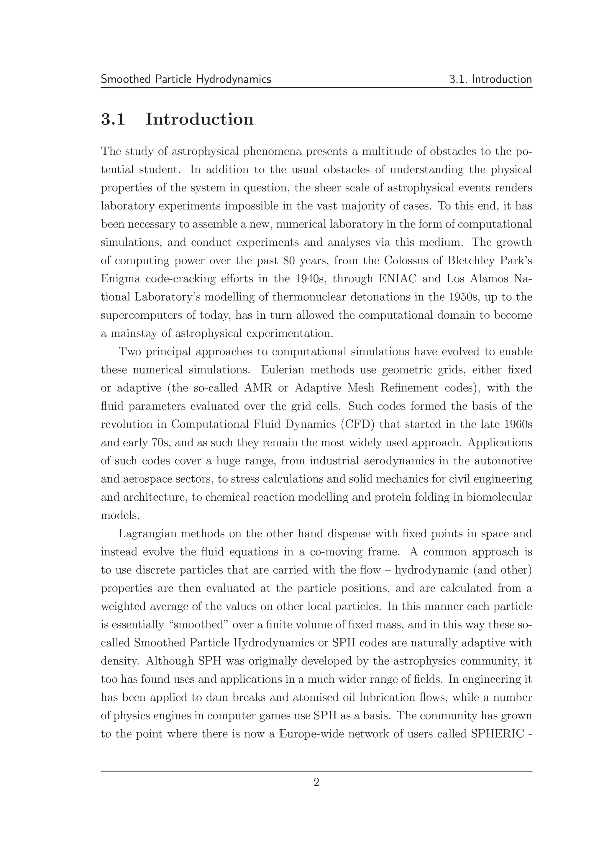
As far as the laws of mathematics refer to real-
ity, they are not certain; and as far as they are
certain, they do not refer to reality.
Albert Einstein
3Smoothed Particle Hydrodynamics
Or: How I Learned to Stop Worrying and Love the Lagrangian*
* With apologies to Drs. Strangelove and Price
1](https://image.slidesharecdn.com/smoothedparticlehydrodynamics-140523203129-phpapp01/75/Smoothed-Particle-Hydrodynamics-1-2048.jpg)
![Smoothed Particle Hydrodynamics 3.3. Fluid Equations
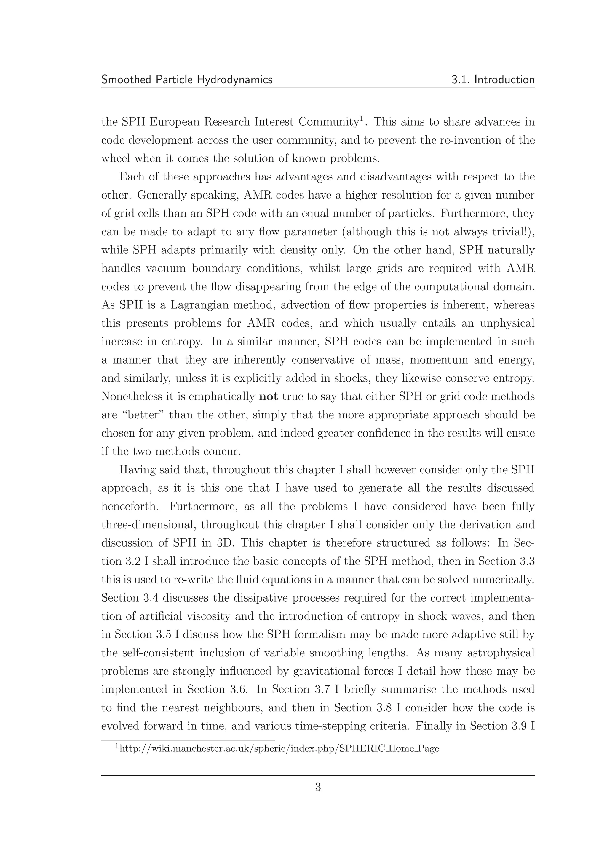
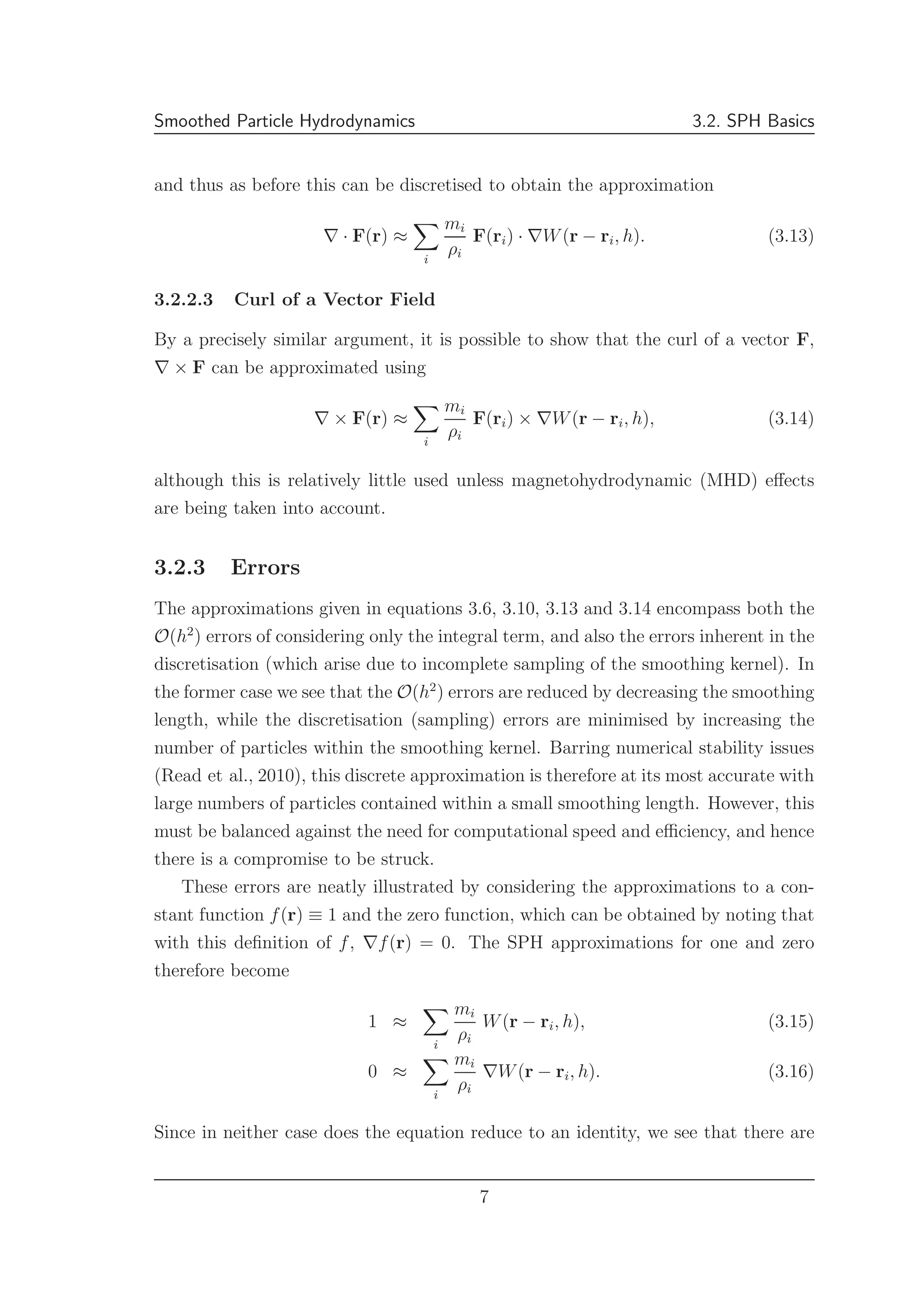
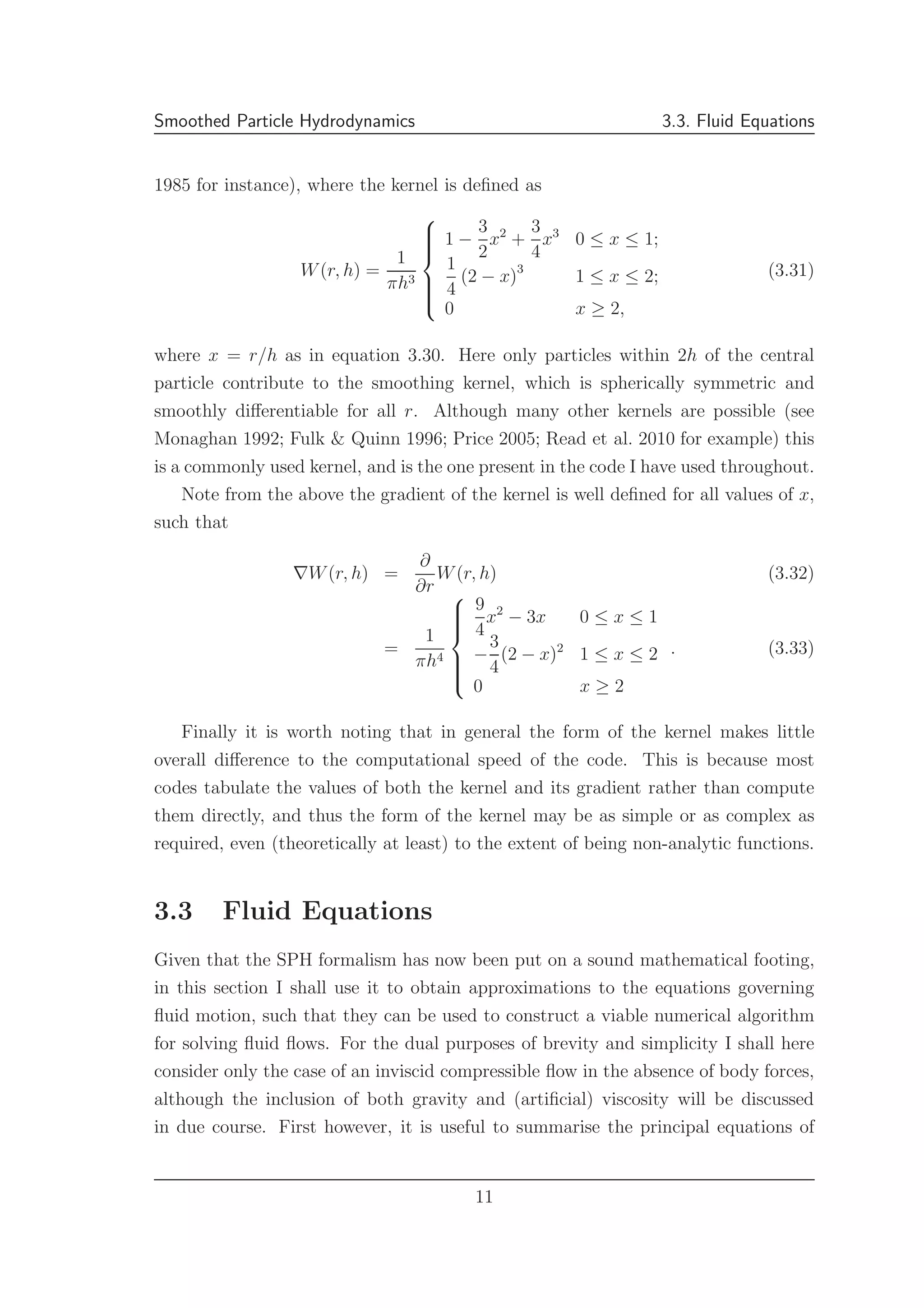
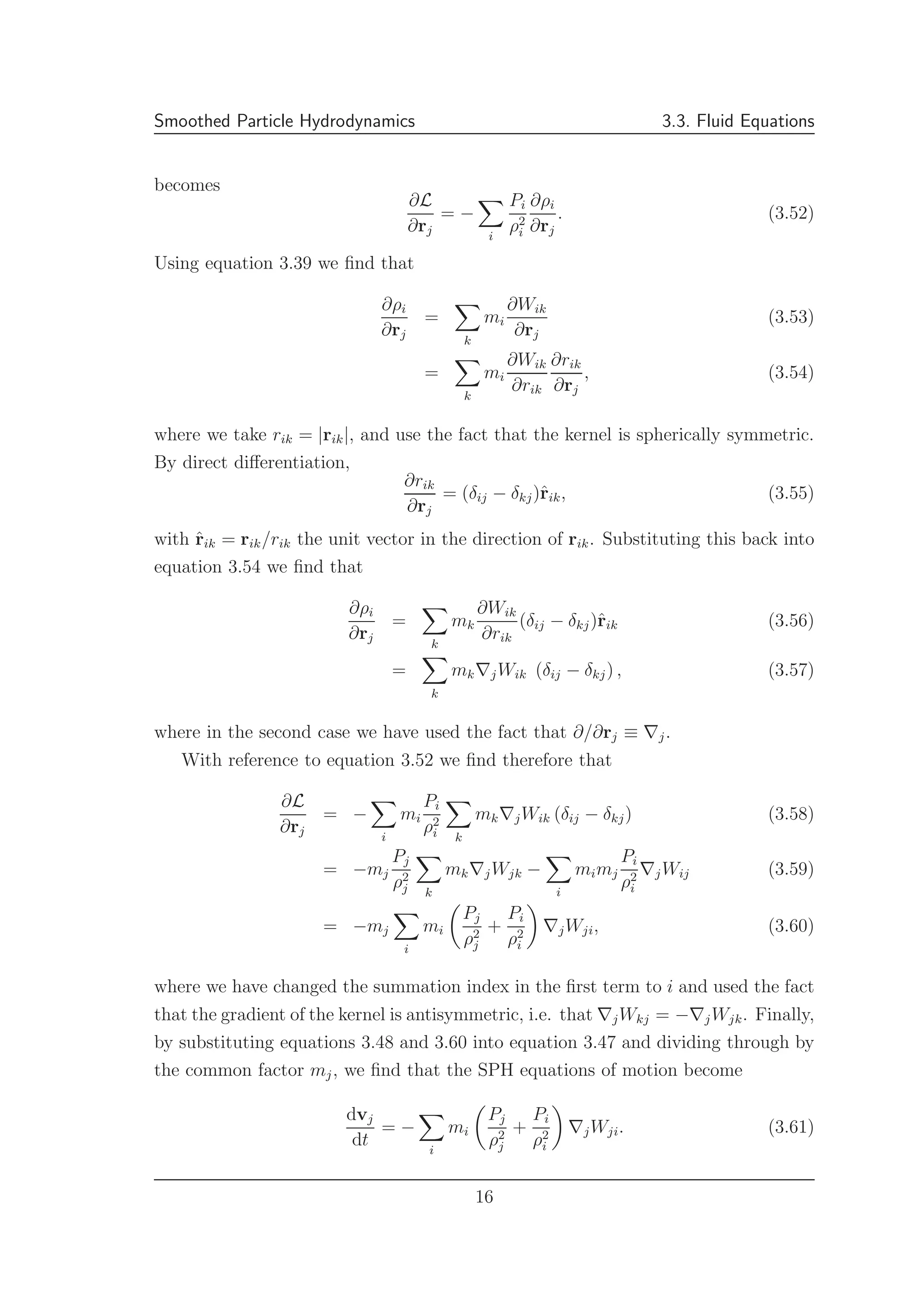
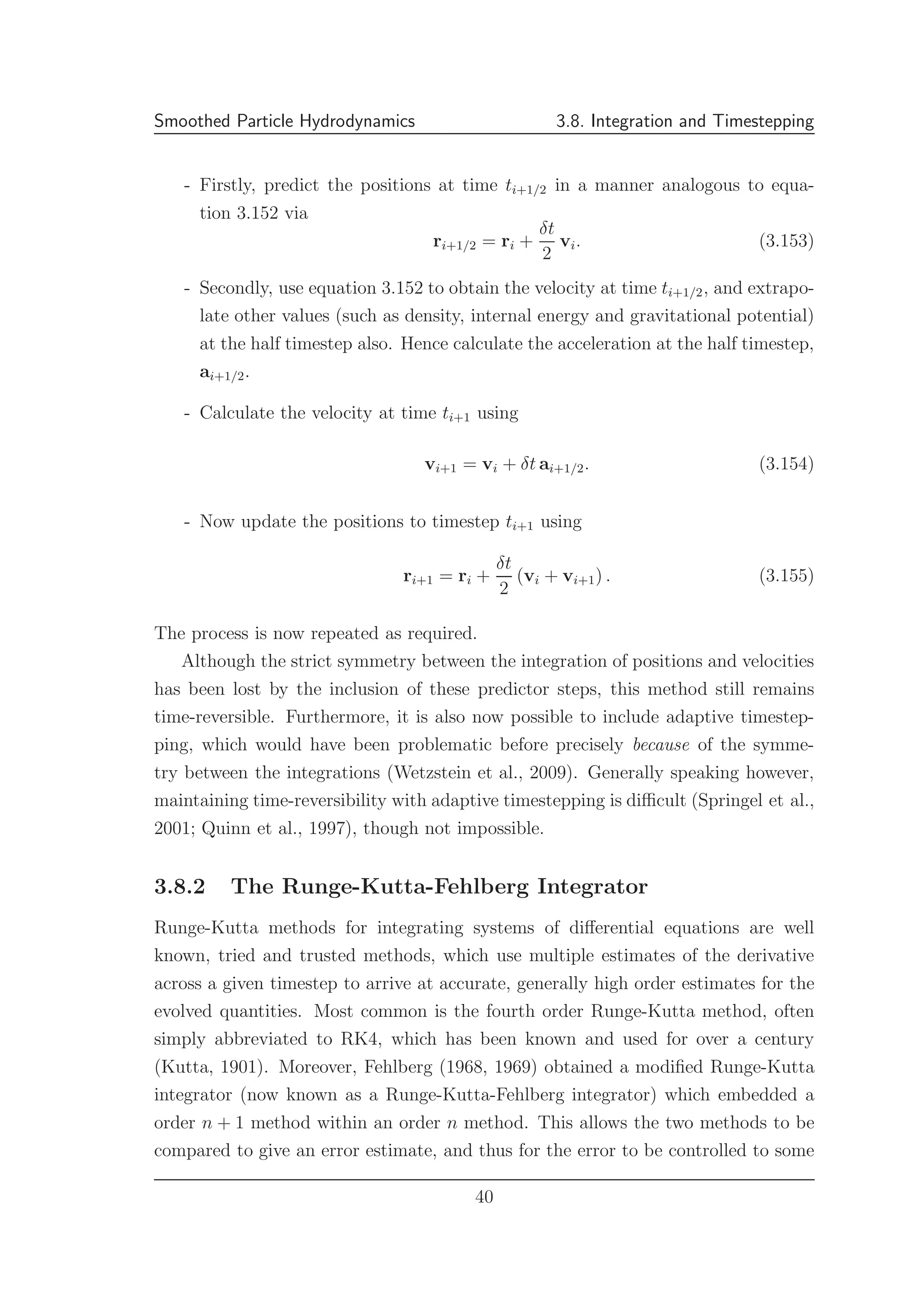
motion in their standard conservative form.
The continuity (conservation of mass) equation is given by
∂ρ
∂t
+ ∇ · (ρv) = 0 (3.34)
where as normal, ρ is the density, t is time and v is velocity.
The Euler equation gives the equations of motion in the case of an inviscid fluid,
and encapsulates the conservation of momentum. In the absence of external (body)
forces it becomes
∂ρv
∂t
+ ∇ · (ρv ⊗ v) + ∇P = 0, (3.35)
where P is the fluid pressure and ⊗ represents the outer or tensor product3
. For
compressible flows it is also necessary to take into account the energy equation, and
as such the conservation of energy is embodied in the following equation;
∂u
∂t
+ ∇ · [(u + P)v] = 0, (3.36)
where u is the specific internal energy and v = |v| is the magnitude of the velocity
vector. Finally it is worth noting that these five equations (there are 3 components
to the momentum equation) contain six unknowns (ρ, the three components of
velocity vx, vy and vz, P and u). Therefore in order to solve the system we require
a further constraint; an equation of state is required. All the analysis I shall present
henceforth uses the ideal gas equation of state, where
P = κ(s)ργ
, (3.37)
= (γ − 1)uρ, (3.38)
where γ is the adiabatic index (the ratio of specific heats), which throughout has
been set to 5/3, and κ(s) is the adiabat, itself a function of the specific entropy s.
In the case of isentropic flows, s and (thus κ) remains constant.
I shall now discuss the SPH formulation of each of the continuity, momentum
and energy equations in turn. Note that again for the purposes of brevity I assume
that the smoothing length is held constant (i.e. ˙h = 0, where the dot denotes the
derivative with respect to time), and is equal for all particles. Individual, variable
smoothing lengths will be discussed in due course. Furthermore, I assume through-
3
The outer product of two vectors may be summarised as A ⊗ B = ABT
= AiBj (in indicial
notation).
12](https://image.slidesharecdn.com/smoothedparticlehydrodynamics-140523203129-phpapp01/75/Smoothed-Particle-Hydrodynamics-12-2048.jpg)
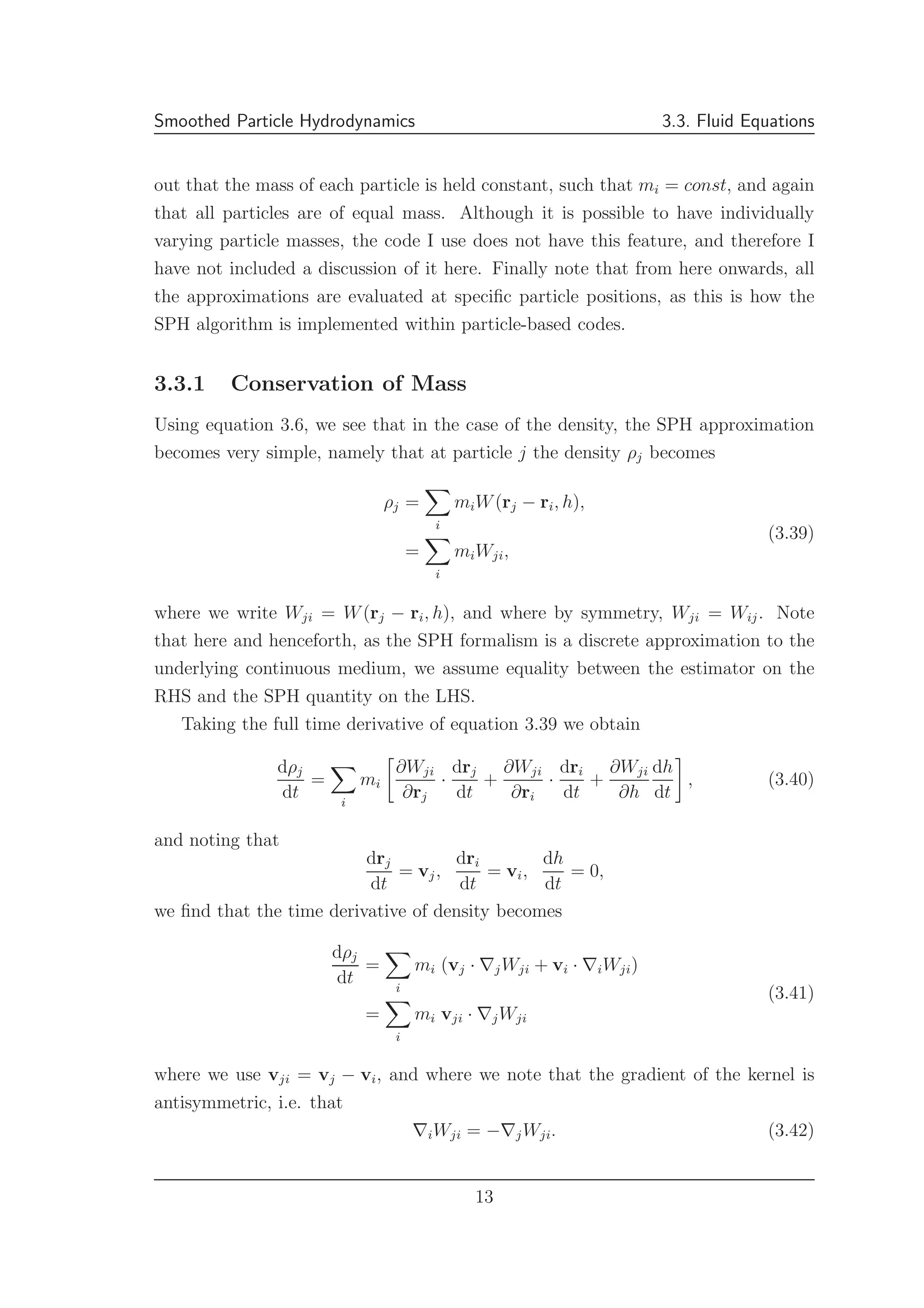
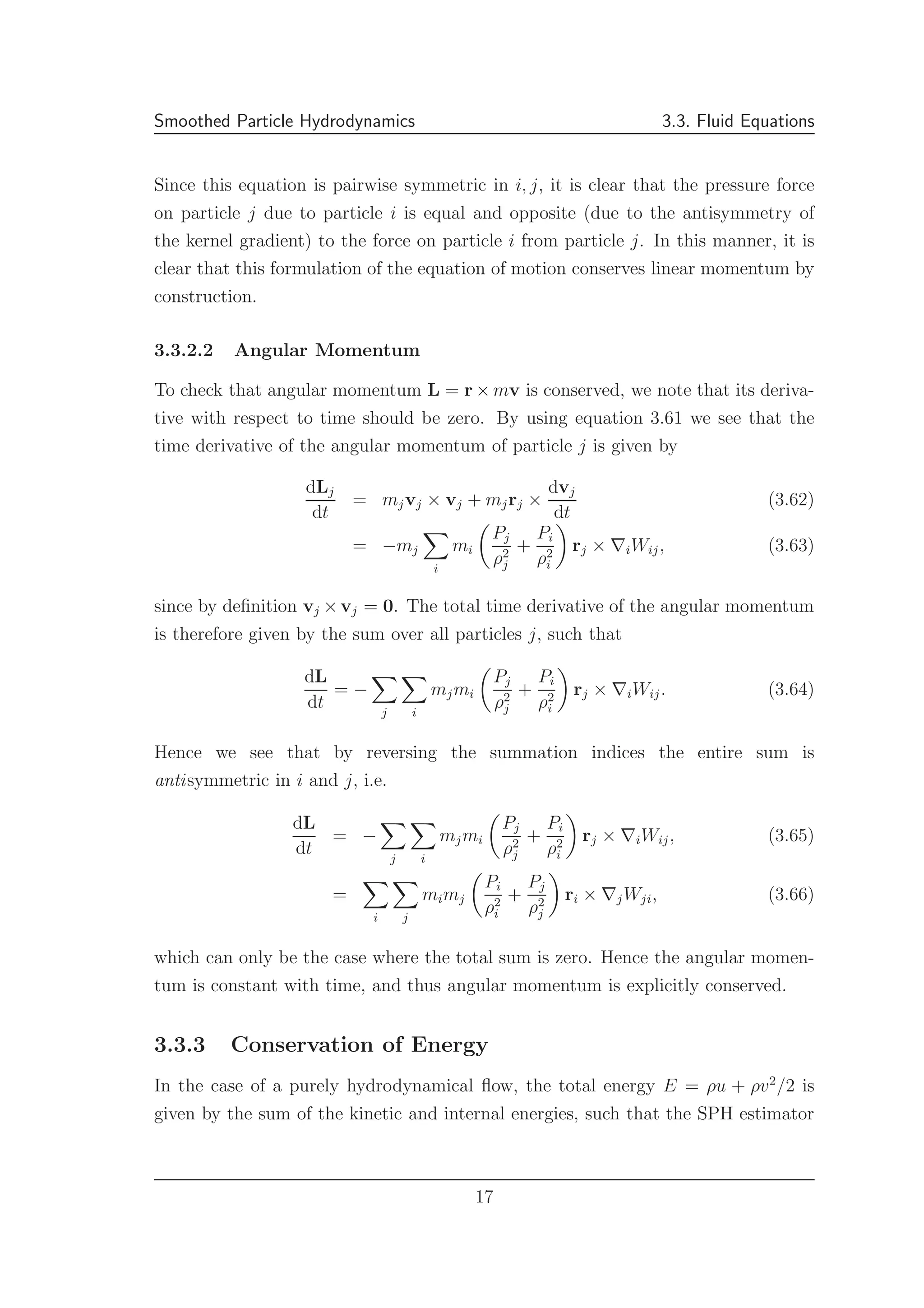
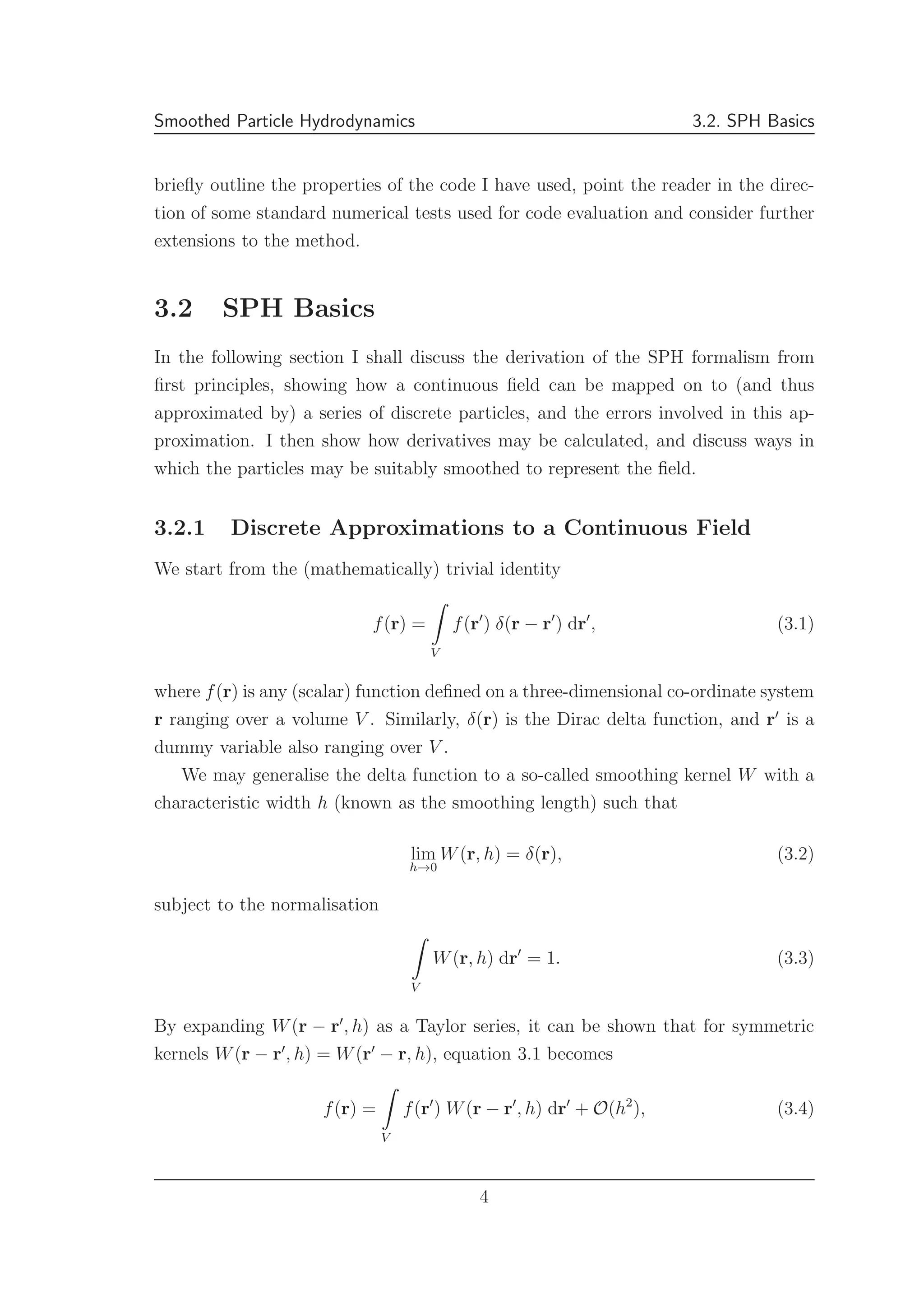
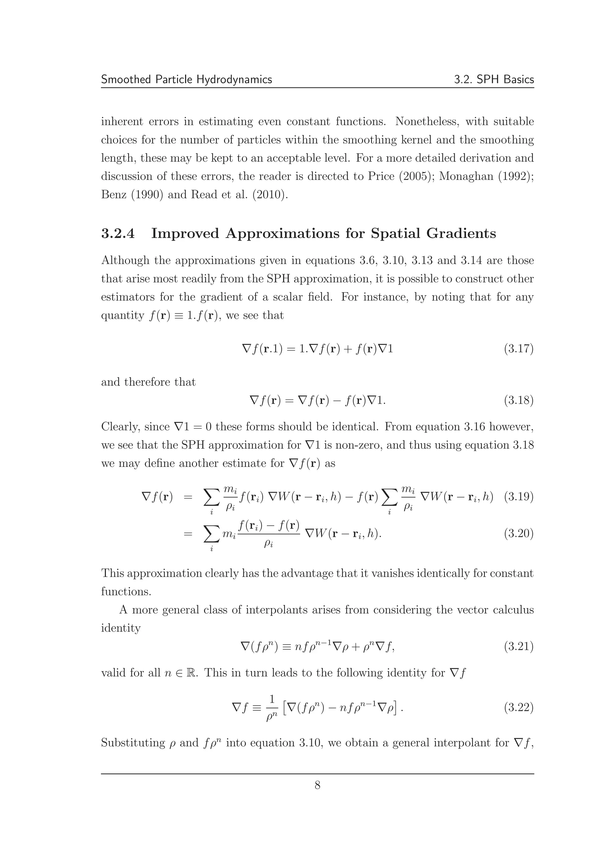
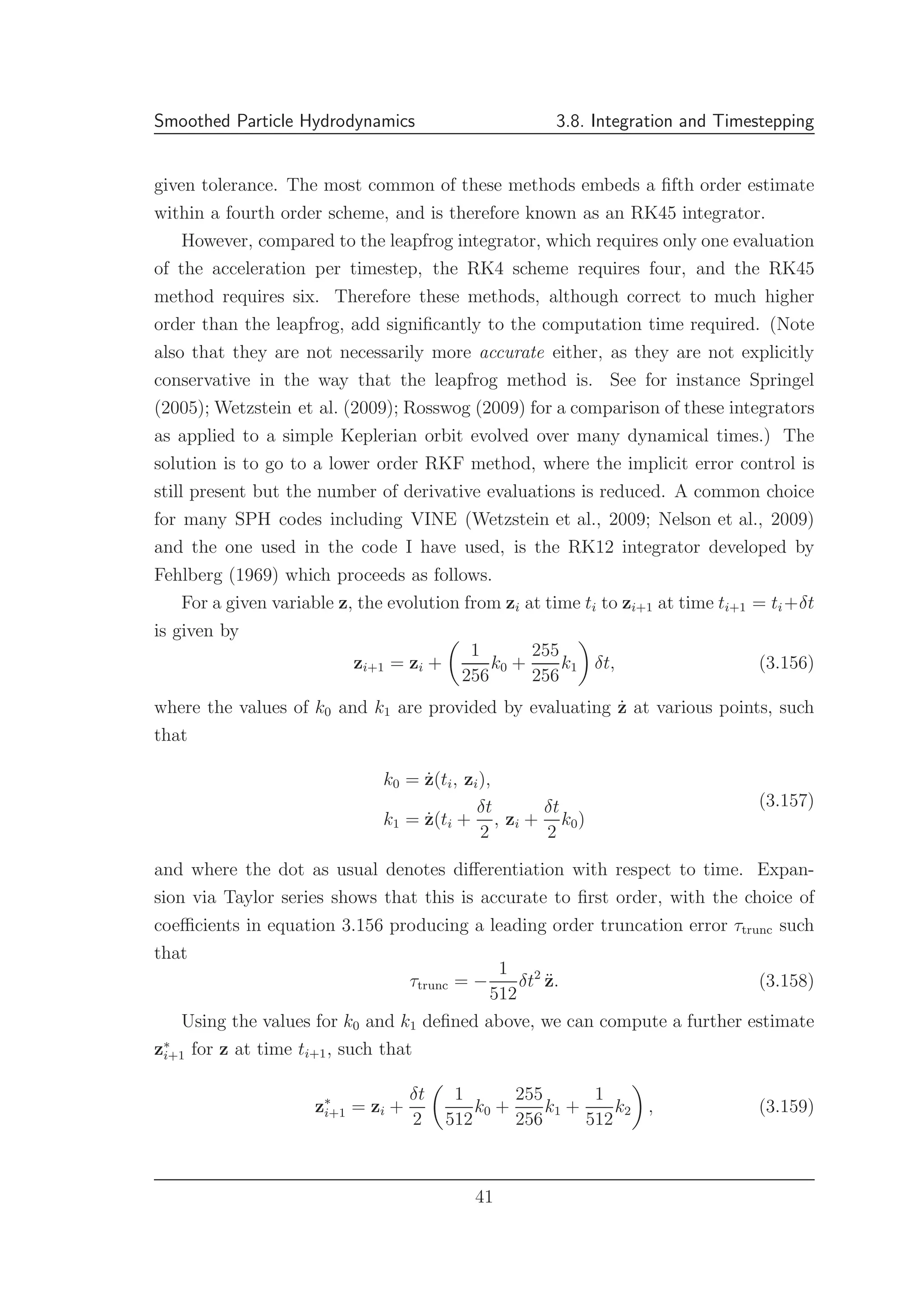
![Smoothed Particle Hydrodynamics 3.5. Variable Smoothing Lengths
where W and ∇W are given by equations 3.31 and 3.33 respectively.
Similarly, there is a correction factor to the momentum equation to allow for
the spatial variation in smoothing lengths. Recall from equation 3.52 that in order
to calculate the spatial variation of the Lagrangian, we need to know the spatial
derivative of the density. Allowing now for variable smoothing lengths and using
equation 3.57, we therefore find that
∂ρj
∂ri
=
k
mk ∇jWji(hj) [δji − δjk] +
∂Wjk(hj)
∂hj
dhj
dρj
∂ρj
∂ri
. (3.108)
By gathering like terms, we find that the correction factor for the spatial derivative
of the density is same as that for the temporal one, namely that
∂ρj
∂ri
=
1
Ωj
k
mk∇iWjk(hj) [δji − δjk] , (3.109)
with the factor Ωj defined as before in equation 3.106.
Following the same derivation as in Section 3.3.2, it is then easy to show that the
acceleration due to hydrodynamic forces with spatially varying smoothing lengths
is given by
dvj
dt
= −
i
mi
Pj
Ωjρ2
j
∇iWji(hj) +
Pi
Ωiρ2
i
∇jWji(hi) . (3.110)
Finally, from equation 3.73, we see that the evolution of the internal energy in the
presence of variable smoothing lengths becomes
duj
dt
=
Pj
Ωjρ2
j i
mivji · ∇Wji(hj). (3.111)
By an analogous process to that described in Section 3.3.3, it is possible to show that
this equation for the evolution of the internal energy is also explicitly conservative of
the total energy of the system, E. The three equations 3.100, 3.110 and 3.111 along
with the relationship between the density and the smoothing length equation 3.98
therefore form a fully consistent, fully conservative SPH formalism with spatially
varying smoothing lengths.
A problem exists however, in that in order to obtain the density, one needs to
know the smoothing length (equation 3.100) and to obtain the smoothing length one
needs to know the density (equation 3.98). In order to resolve this, this pair of equa-
28](https://image.slidesharecdn.com/smoothedparticlehydrodynamics-140523203129-phpapp01/75/Smoothed-Particle-Hydrodynamics-28-2048.jpg)

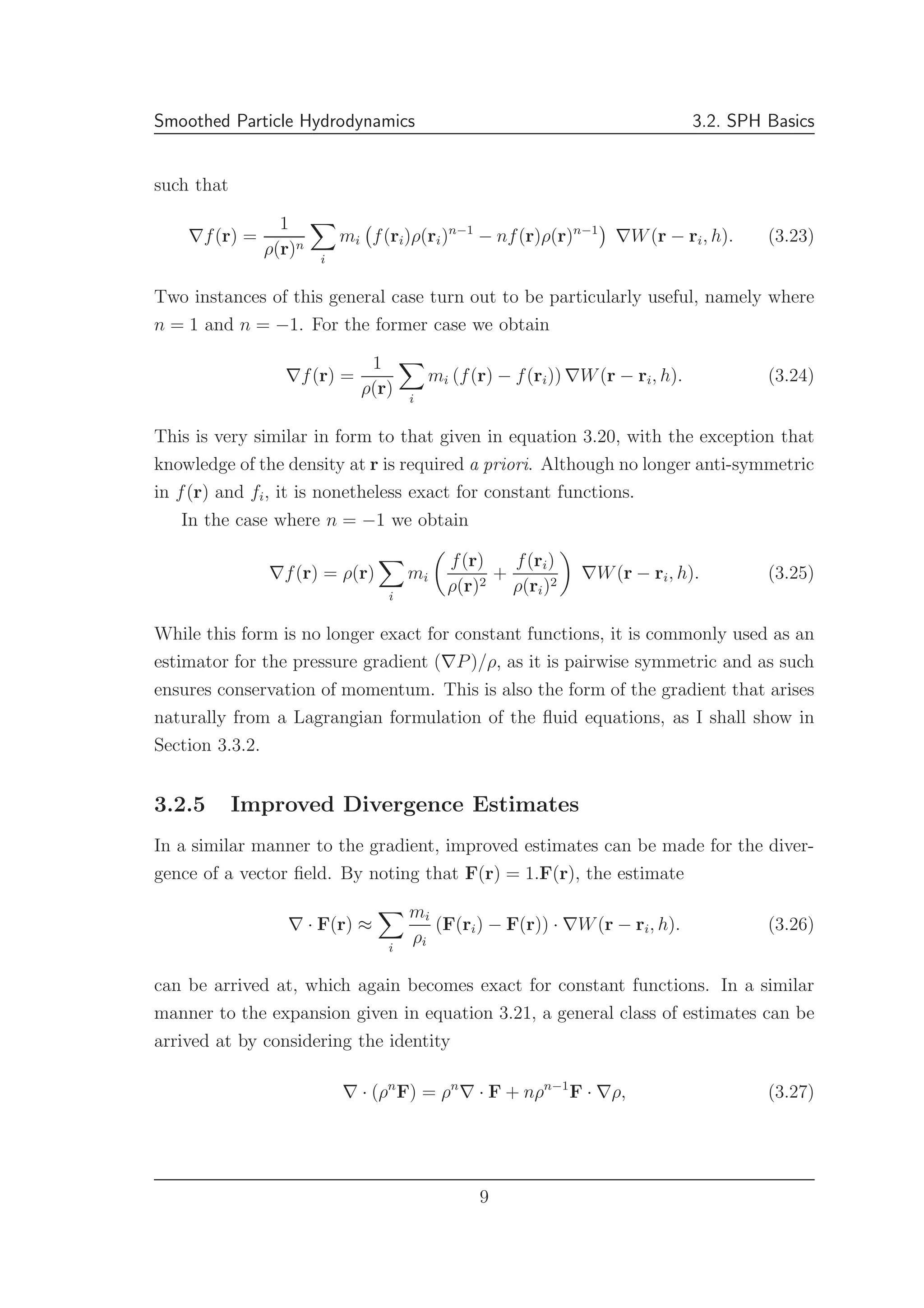
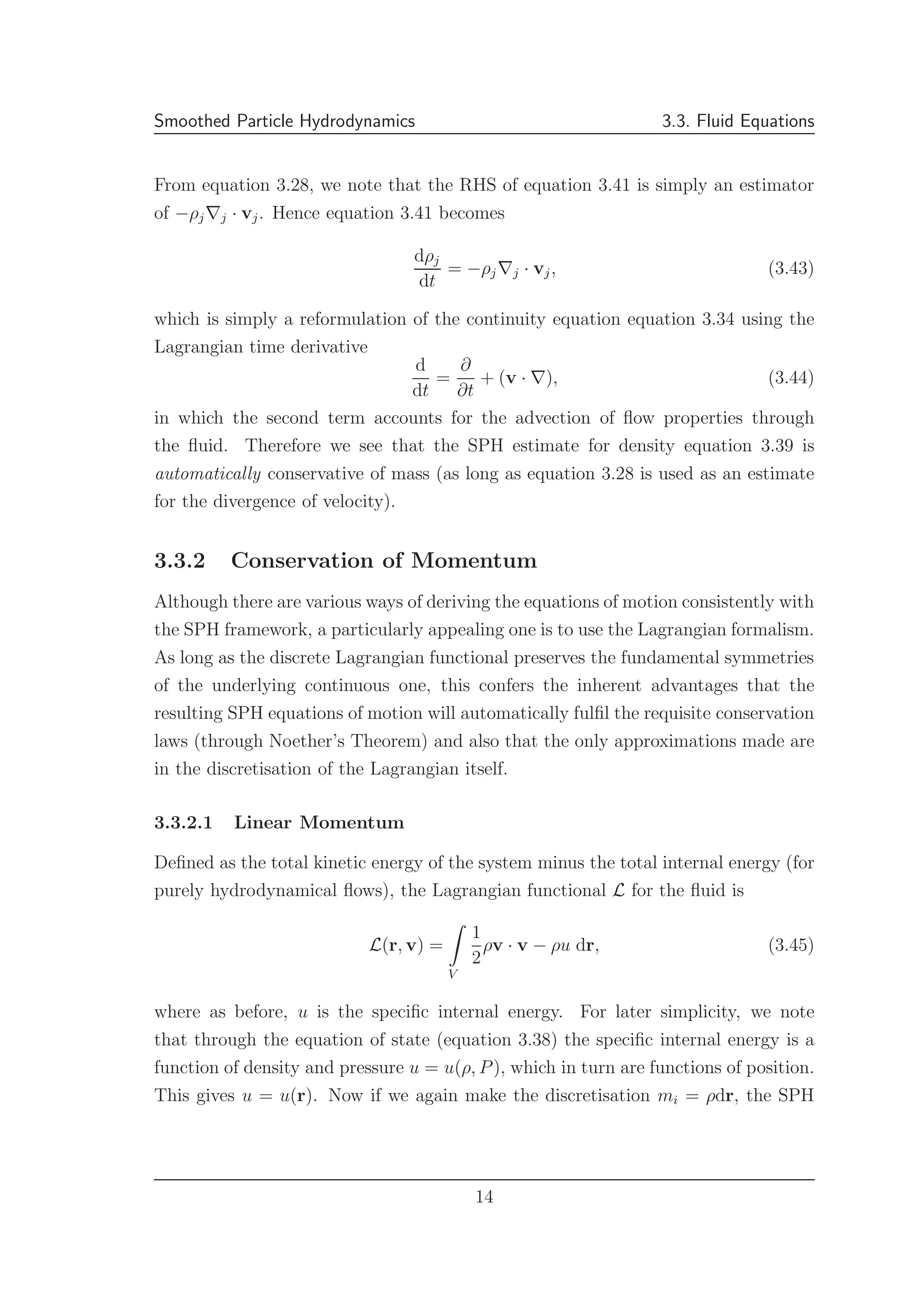
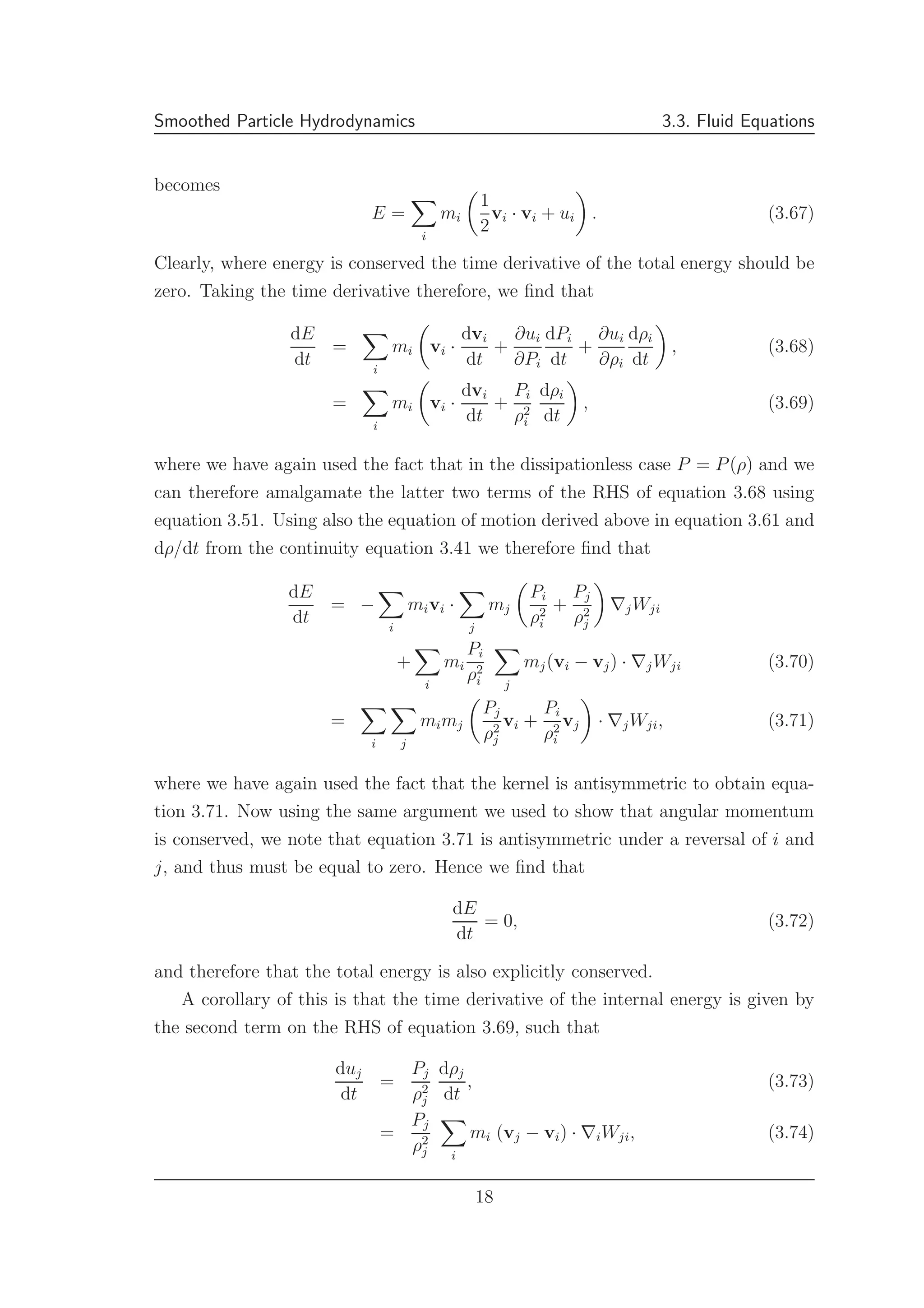
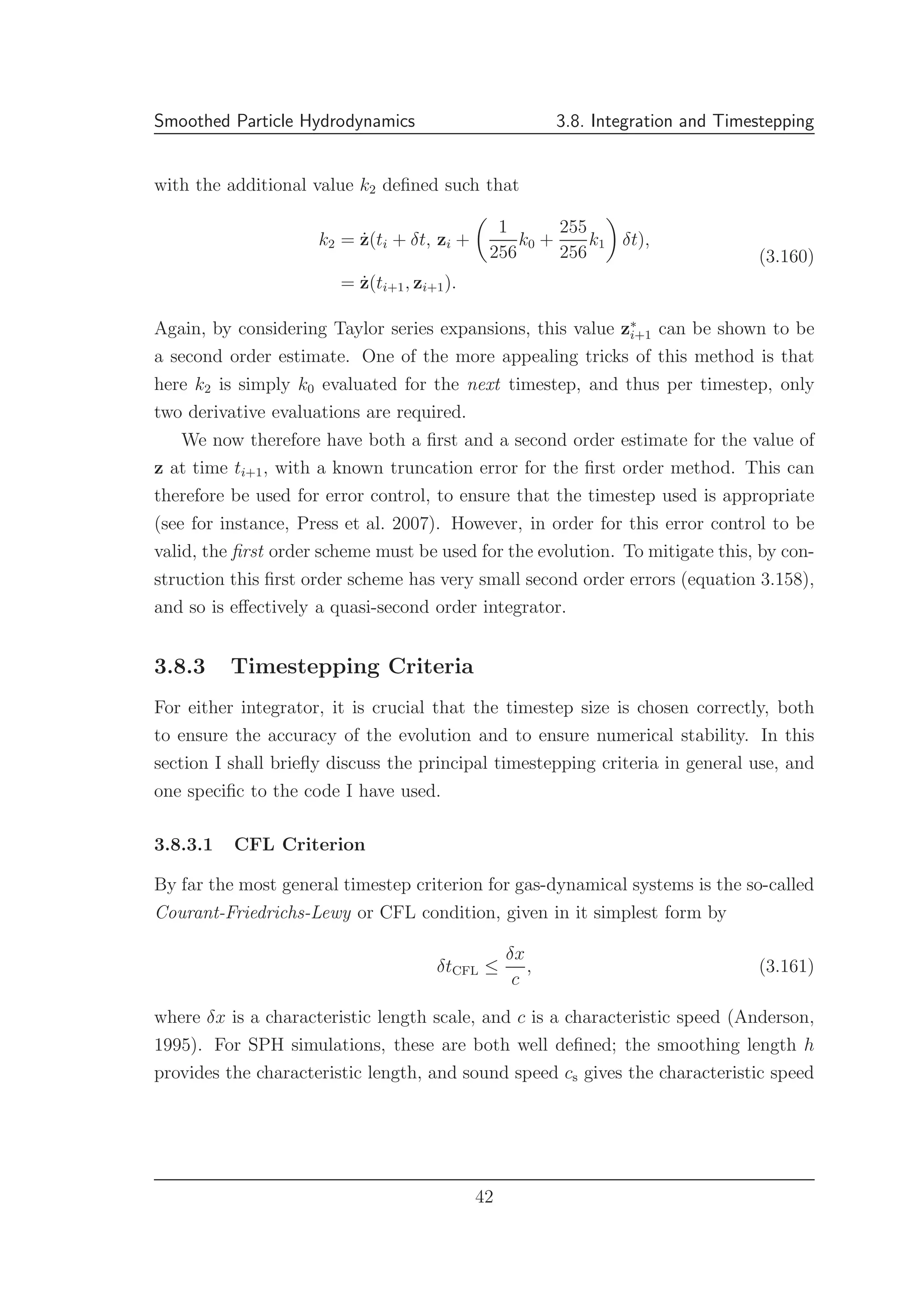
![Smoothed Particle Hydrodynamics 3.6. Including Gravity
which becomes
mj
dvj
dt
=
∂Lgrav
∂rj
. (3.123)
Using equations 3.117 and 3.120 we therefore find that the spatial derivative of the
gravitational Lagrangian becomes
∂Lgrav
∂rj
= −
G
2 i k
mimk
∂φik(hi)
∂rj
(3.124)
= −
G
2 i k
mimk ∇jφik(hi) +
∂φik(hi)
∂hi
∂hi
∂rj
. (3.125)
Here we see that in the case of fixed smoothing (and therefore softening) lengths,
∂hi/∂rk = 0, and thus we only require the first term to determine the effects of
gravity. The second term is therefore a correction term to allow for spatial variation
in h.
As before, using the method of equations 3.54 to 3.57 the spatial gradient be-
comes
∂Lgrav
∂rj h
= −
G
2 i k
mimk ∇jφik(hi) [δij − δkj] , (3.126)
= −
G
2
mj
k
mk∇jφjk(hj) +
G
2 i
mimj∇jφij(hi). (3.127)
Now by changing the summation index of the first term to i, and noting again that
the kernel is antisymmetric we obtain
∂Lgrav
∂rj h
= −
G
2
mj
i
mi (∇jφji(hj) + ∇jφji(hi)) , (3.128)
which therefore encapsulates the effects of gravity in the case of constant smoothing
lengths.
If we now consider the second term in equation 3.125 and self-consistently correct
for spatial variation in the smoothing length, we find that
∂Lgrav
∂rj corr
= −
G
2 i k
mimk
∂φik(hi)
∂hi
dhi
dρi
∂ρi
∂rj
. (3.129)
32](https://image.slidesharecdn.com/smoothedparticlehydrodynamics-140523203129-phpapp01/75/Smoothed-Particle-Hydrodynamics-32-2048.jpg)
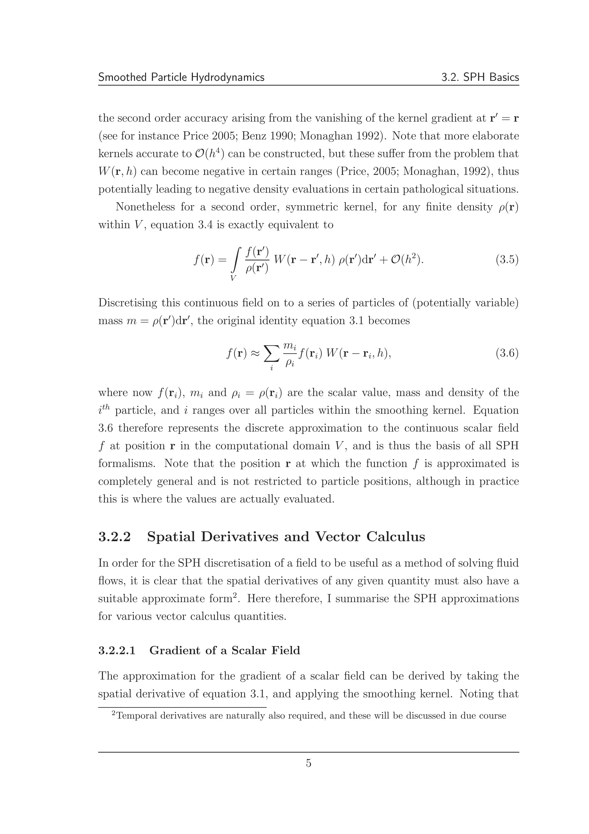
![Smoothed Particle Hydrodynamics 3.6. Including Gravity
By substituting equation 3.109 into the above we find that
∂Lgrav
∂rj corr
= −
G
2 i k
mimk
∂φik(hi)
∂hi
dhi
dρi
1
Ωi
l
ml∇jWil(hl)[δij − δlj] (3.130)
= −
G
2
mj
k
mk
∂φjk
∂hj
dhj
dρj
1
Ωj
l
ml∇jWjl(hl)
+
G
2 i k
∂φik(hi)
∂hi
1
Ωi
mj∇jWij(hi).
(3.131)
Now by changing the summation index of the second sum in the first term of equa-
tion 3.131 to i, defining a new quantity ξp such that
ξp =
dhp
dρp q
mq
∂φpq(hp)
∂hp
, (3.132)
and using the antisymmetry property of the gradient of the smoothing kernel, we
see that the correction term reduces to
∂Lgrav
∂rj corr
= −
G
2
mj
i
mi
ξj
Ωj
∇jWji(hj) +
ξi
Ωi
∇jWji(hi) . (3.133)
Finally, using equation 3.123 and by incorporating the effects of gravity into the
equations of motion for a hydrodynamic flow with artificial viscosity (while self-
consistently allowing for variable smoothing lengths) we find that the full equations
of motion become
dvj
dt
= −
i
mi
Pj
Ωjρ2
j
∇jWji(hj) +
Pi
Ωiρ2
i
∇jWji(hi) + Πji
∇jWji(hj) + ∇jWji(hi)
2
−
G
2 i
mi (∇jφji(hj) + ∇jφji(hj)) (3.134)
−
G
2 i
mi
ξj
Ωj
∇jWji(hj) +
ξi
Ωi
∇jWji(hi) ,
with Ωi and ξi defined as per equations 3.106 and 3.132 respectively6
. As in the case
for the pure hydrodynamic flow, the use of a Lagrangian in deriving these equations
ensures the explicit conservation of both linear and angular momentum, which is
also clear from the pairwise symmetry present in all terms in the above equation.
6
Note that for consistency, the artificial viscosity term Πji uses the average value of the smooth-
ing lengths hji = (hj + hi)/2 in its definition of µji (equation 3.83).
33](https://image.slidesharecdn.com/smoothedparticlehydrodynamics-140523203129-phpapp01/75/Smoothed-Particle-Hydrodynamics-33-2048.jpg)

This document discusses smoothed particle hydrodynamics (SPH), a Lagrangian numerical method for simulating fluid flows. SPH uses discrete particles that move with the fluid and sample hydrodynamic properties by averaging values over neighboring particles. The document outlines the basic concepts of SPH, including how it approximates continuous fields with discrete particles and calculates spatial derivatives. It also discusses how SPH can be used to model astrophysical phenomena through numerical simulations since laboratory experiments are often impossible at astrophysical scales.


![Vibe Coding vs. Spec-Driven Development [Free Meetup]](https://cdn.slidesharecdn.com/ss_thumbnails/vibecodingvsspecdrivendevelopment-251209105622-43f455e7-thumbnail.jpg?width=640&height=640&fit=bounds)


