Lecture1 for industrial organization for undergrad
1.
ECON 404 A:
IndustrialOrganization & Price
Analysis
Spring Quarter 2020
Lecture 1
March 31, 2020
Yuya Takahashi
1
2.
Information
• Lectures: Tuesdaysand Thursdays from 1:30-3:20
• Classroom: Zoom
• Office Hours: After class, or by appointment
• Office: Savery Hall, room 329
• Contact: ytakahas@uw.edu
• Prerequisite: intermediate microeconomics, calculus, basic econometrics
• Course webpage:
https://sites.google.com/site/yuyasweb/teaching/competition
•
2
3.
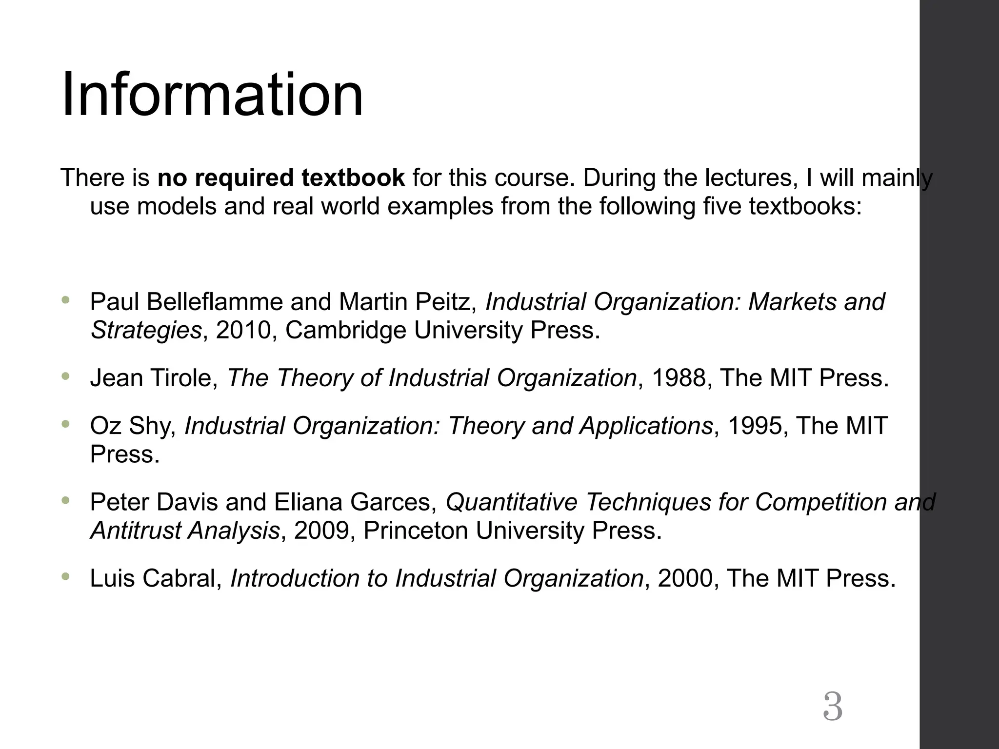
Information
There is norequired textbook for this course. During the lectures, I will mainly
use models and real world examples from the following five textbooks:
Paul Belleflamme and Martin Peitz, Industrial Organization: Markets and
Strategies, 2010, Cambridge University Press.
Jean Tirole, The Theory of Industrial Organization, 1988, The MIT Press.
Oz Shy, Industrial Organization: Theory and Applications, 1995, The MIT
Press.
Peter Davis and Eliana Garces, Quantitative Techniques for Competition and
Antitrust Analysis, 2009, Princeton University Press.
Luis Cabral, Introduction to Industrial Organization, 2000, The MIT Press.
3
4.
Exam and Grading
•There will be one midterm exam, three problem sets (both
analytical and empirical exercises) and one final exam.
Each of these exams and problem sets accounts for 20% of
the course grade.
• Homework assignments: There will be three problem sets.
Students are encouraged to work as a group, but each
student should write her/his own answer.
• Due dates for assignments:
Homework I: Thursday, April 23
Homework II: Tuesday, May 19
Homework III: Thursday, June 4
4
5.
Tools
• Why dowe need a model?
• Why do we need game theory?
• Why do we use data? How?
5
Producer’s Problem
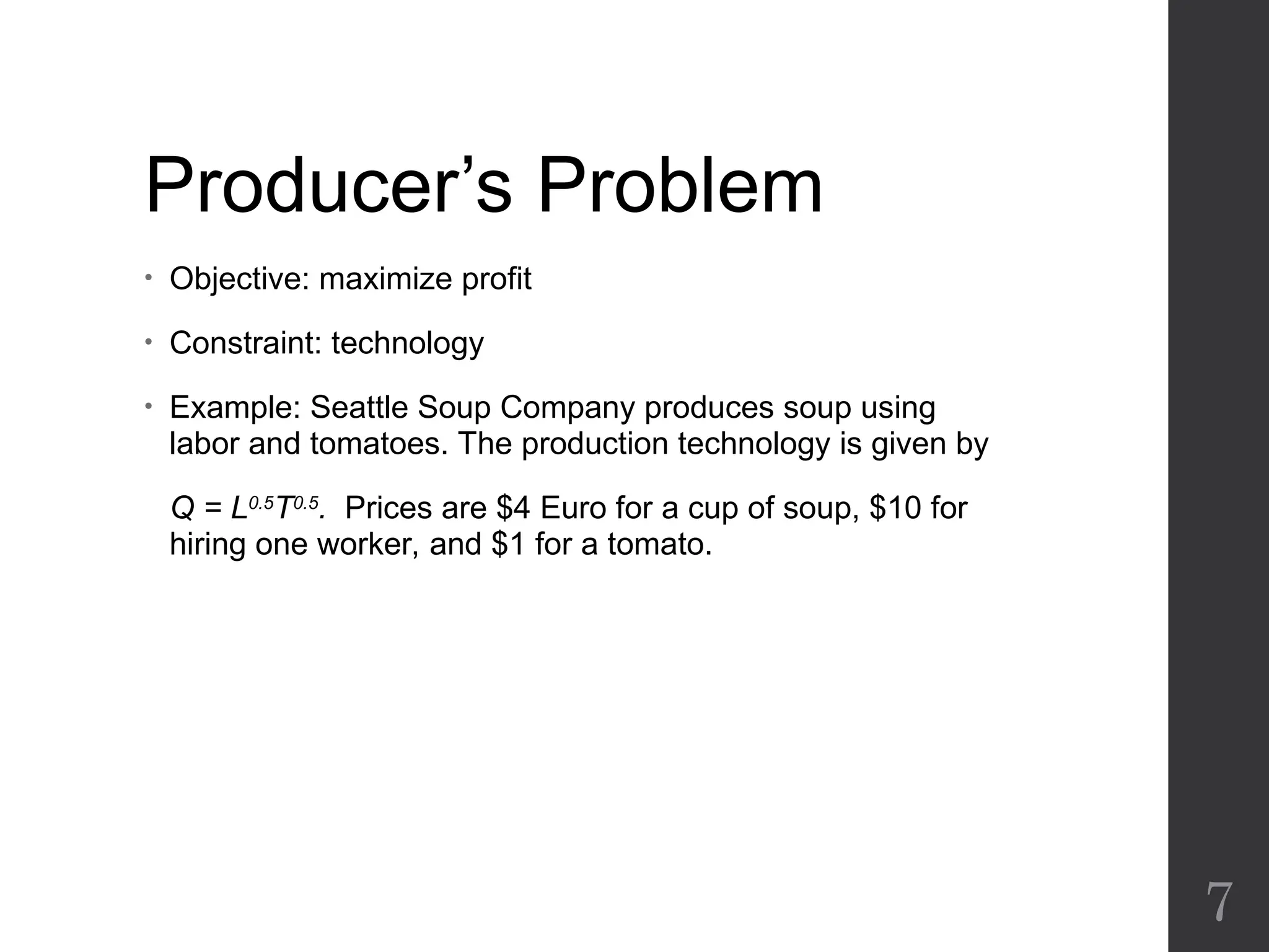
• Objective:maximize profit
• Constraint: technology
• Example: Seattle Soup Company produces soup using
labor and tomatoes. The production technology is given by
Q = L0.5
T0.5
. Prices are $4 Euro for a cup of soup, $10 for
hiring one worker, and $1 for a tomato.
7
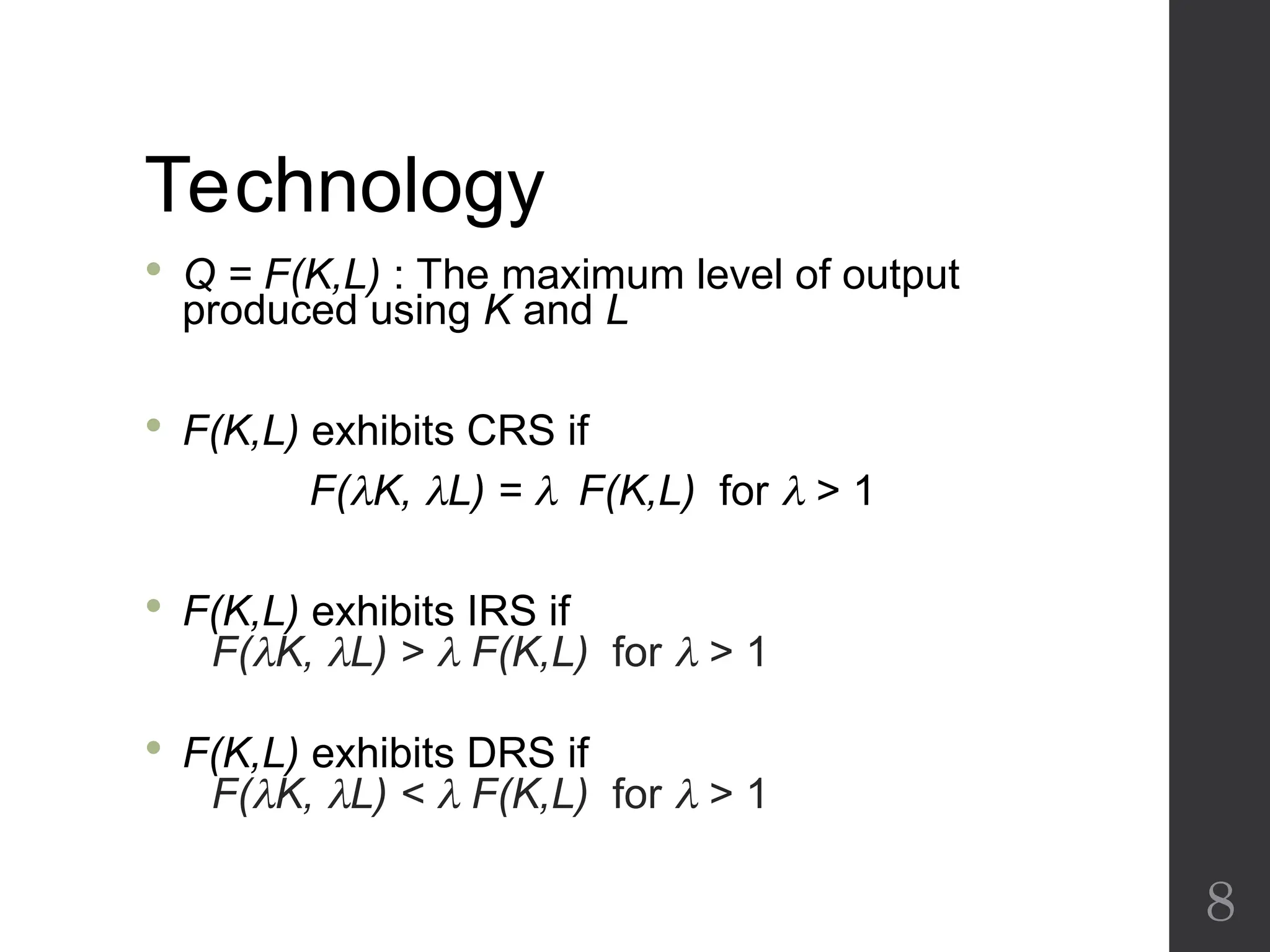
8.
Technology
Q =F(K,L) : The maximum level of output
produced using K and L
F(K,L) exhibits CRS if
F(K, L) = F(K,L) for > 1
F(K,L) exhibits IRS if
F(K, L) > F(K,L) for > 1
F(K,L) exhibits DRS if
F(K, L) < F(K,L) for > 1
8
9.
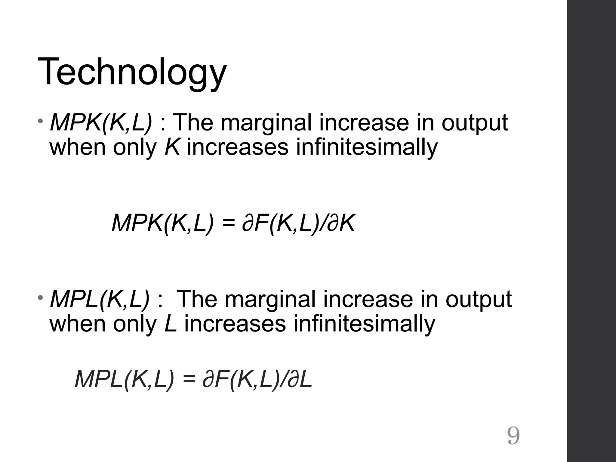
Technology
• MPK(K,L) :The marginal increase in output
when only K increases infinitesimally
MPK(K,L) = ∂F(K,L)/∂K
• MPL(K,L) : The marginal increase in output
when only L increases infinitesimally
MPL(K,L) = ∂F(K,L)/∂L
9
10.
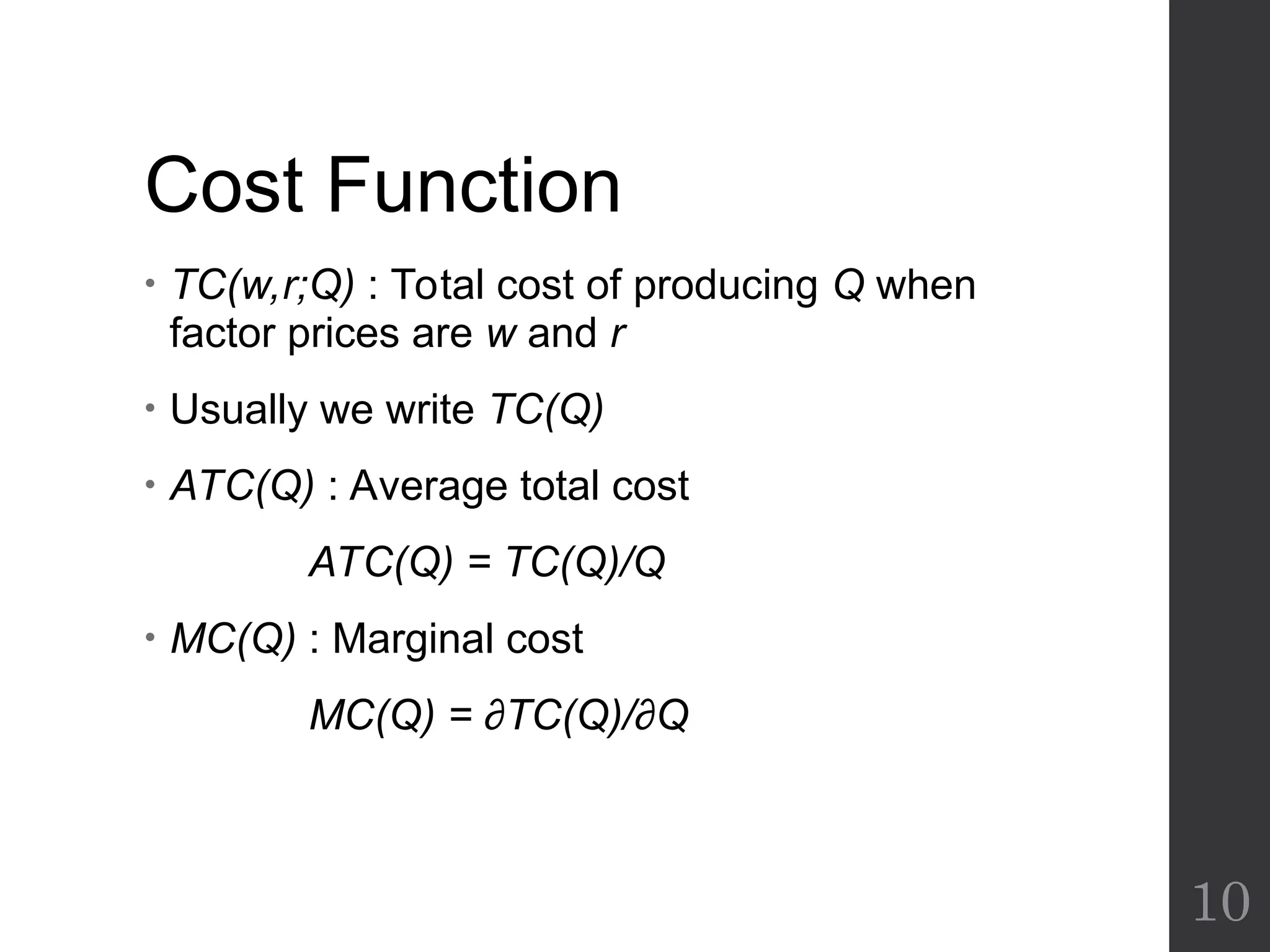
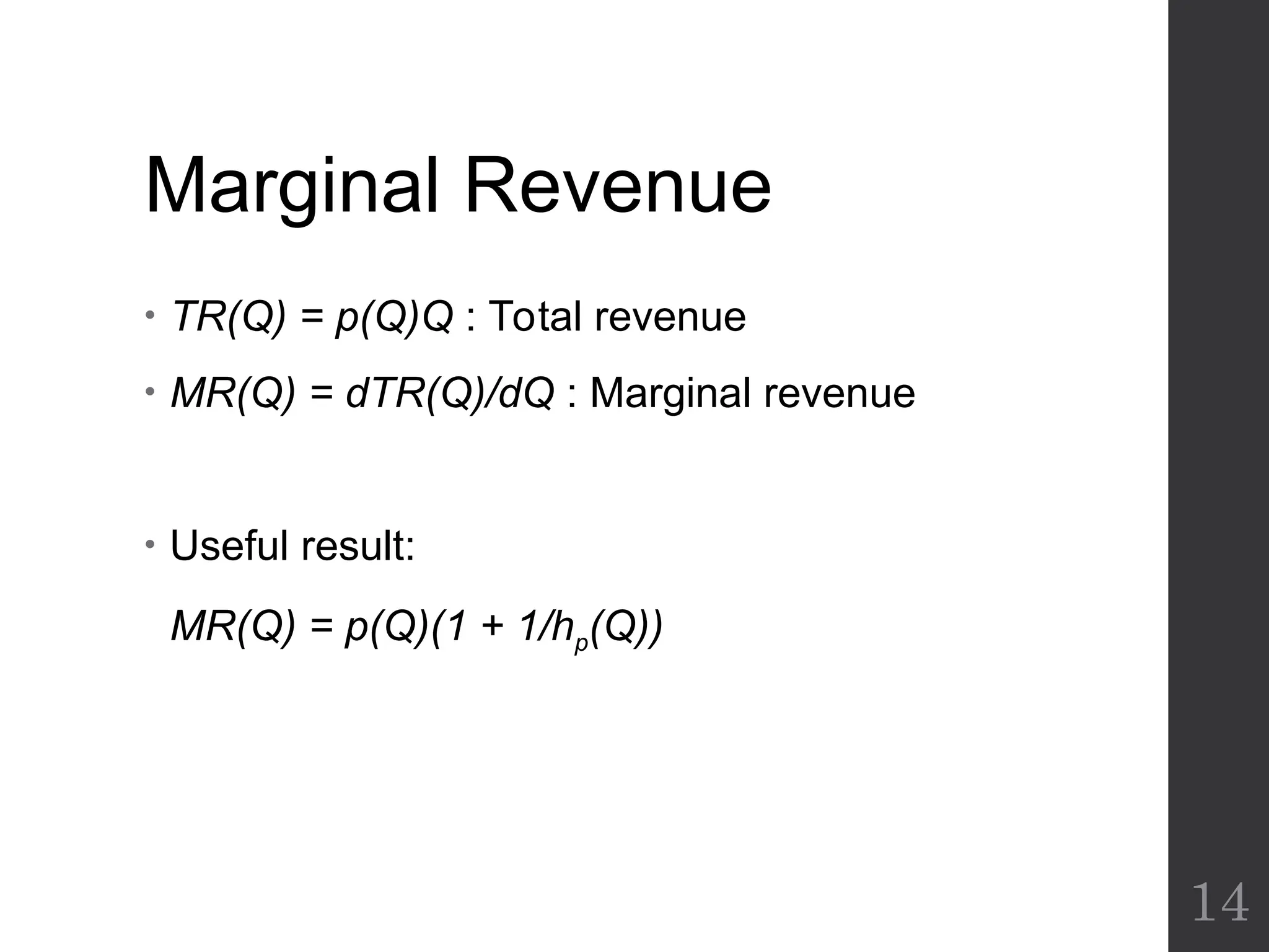
Cost Function
• TC(w,r;Q): Total cost of producing Q when
factor prices are w and r
• Usually we write TC(Q)
• ATC(Q) : Average total cost
ATC(Q) = TC(Q)/Q
• MC(Q) : Marginal cost
MC(Q) = ∂TC(Q)/∂Q
10
11.
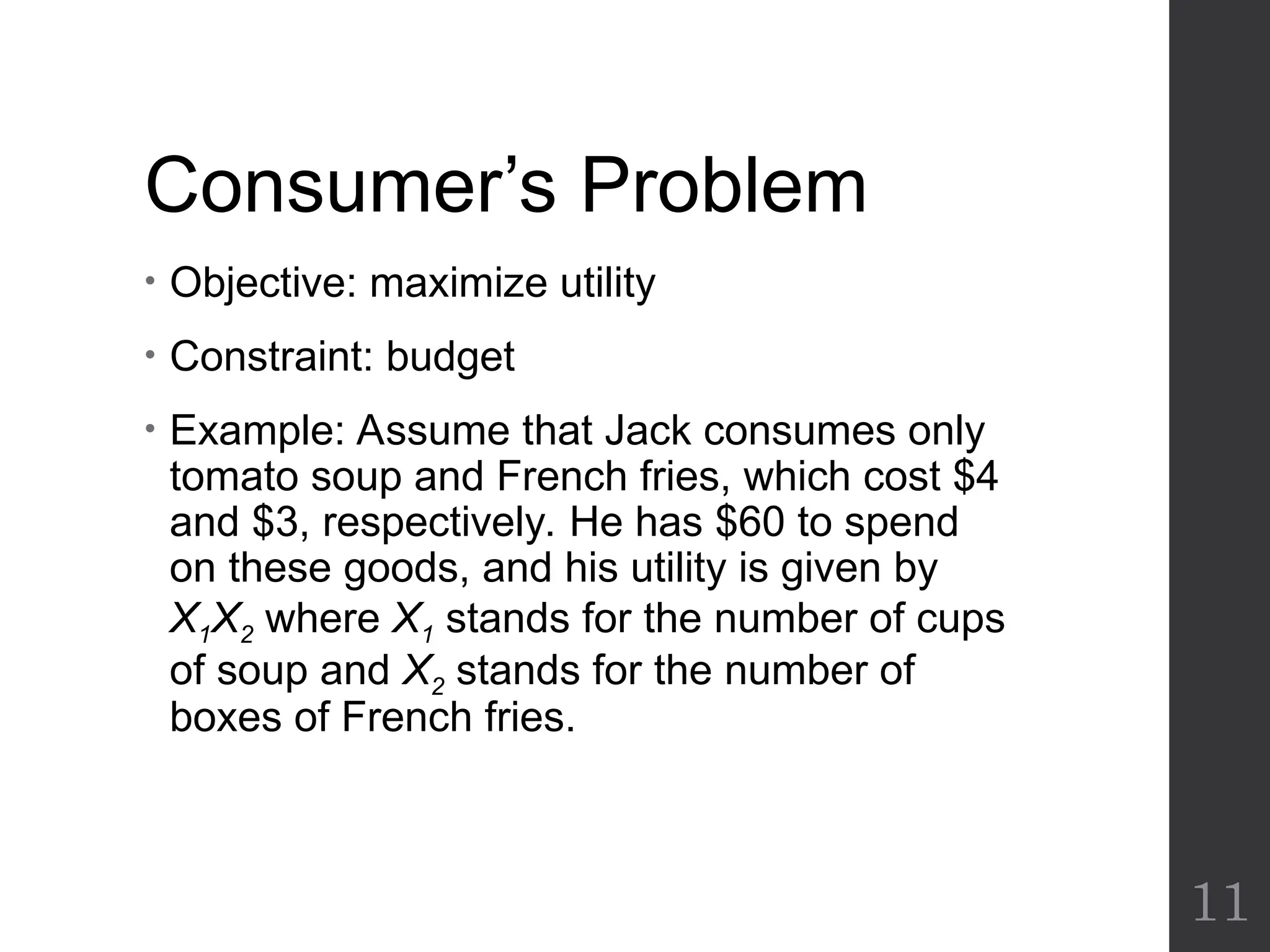
Consumer’s Problem
• Objective:maximize utility
• Constraint: budget
• Example: Assume that Jack consumes only
tomato soup and French fries, which cost $4
and $3, respectively. He has $60 to spend
on these goods, and his utility is given by
X1X2 where X1 stands for the number of cups
of soup and X2 stands for the number of
boxes of French fries.
11
12.
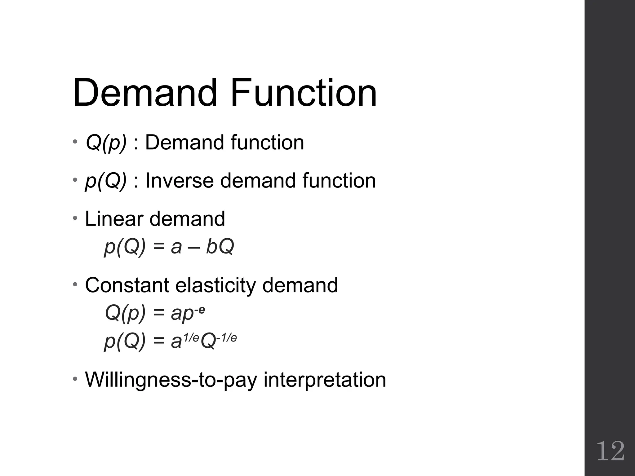
Demand Function
• Q(p): Demand function
• p(Q) : Inverse demand function
• Linear demand
p(Q) = a – bQ
• Constant elasticity demand
Q(p) = ap-e
p(Q) = a1/e
Q-1/e
• Willingness-to-pay interpretation
12
13.
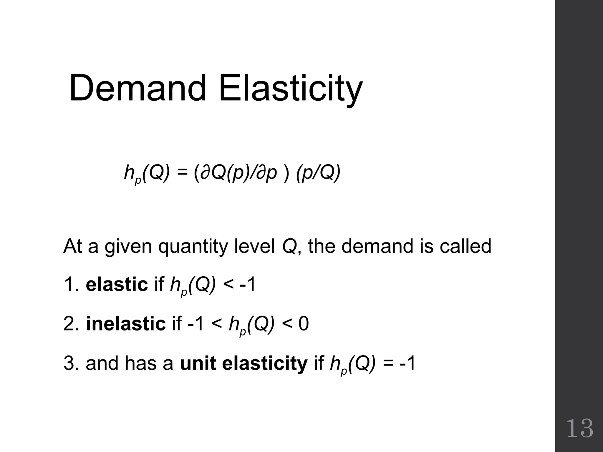
Demand Elasticity
hp(Q) =(∂Q(p)/∂p ) (p/Q)
At a given quantity level Q, the demand is called
1. elastic if hp(Q) < -1
2. inelastic if -1 < hp(Q) < 0
3. and has a unit elasticity if hp(Q) = -1
13
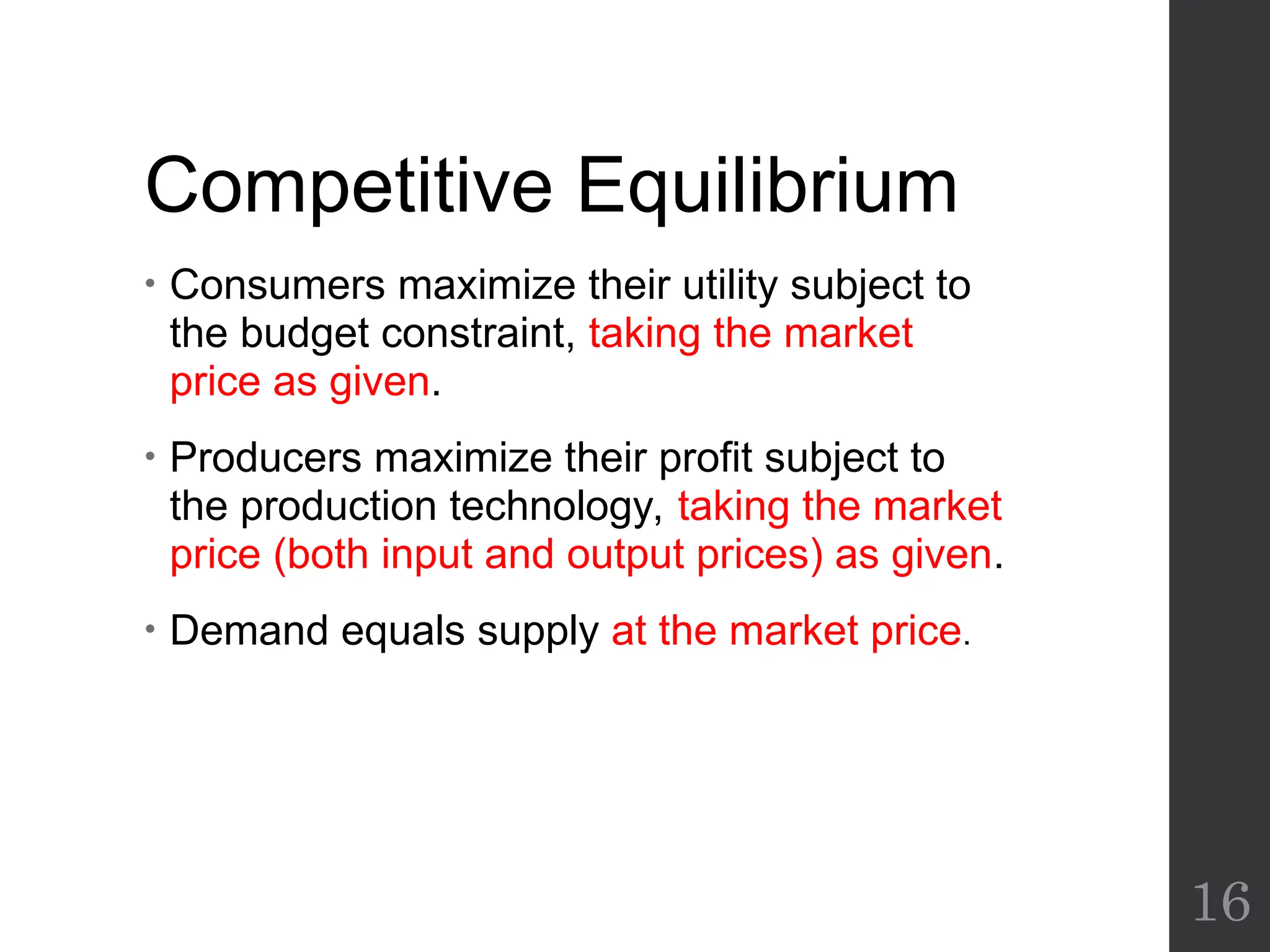
Competitive Equilibrium
• Consumersmaximize their utility subject to
the budget constraint, taking the market
price as given.
• Producers maximize their profit subject to
the production technology, taking the market
price (both input and output prices) as given.
• Demand equals supply at the market price.
16
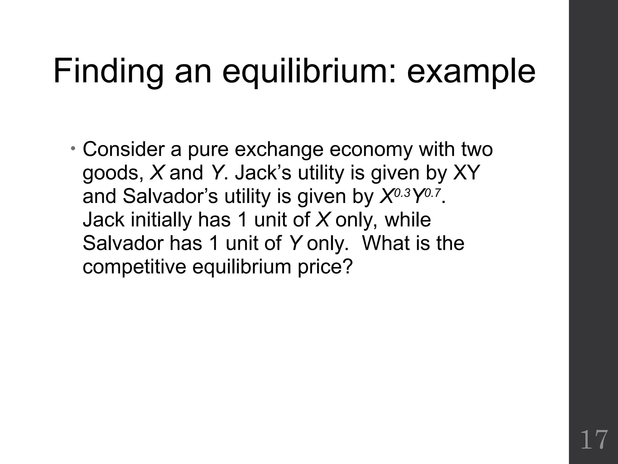
17.
Finding an equilibrium:example
• Consider a pure exchange economy with two
goods, X and Y. Jack’s utility is given by XY
and Salvador’s utility is given by X0.3
Y0.7
.
Jack initially has 1 unit of X only, while
Salvador has 1 unit of Y only. What is the
competitive equilibrium price?
17
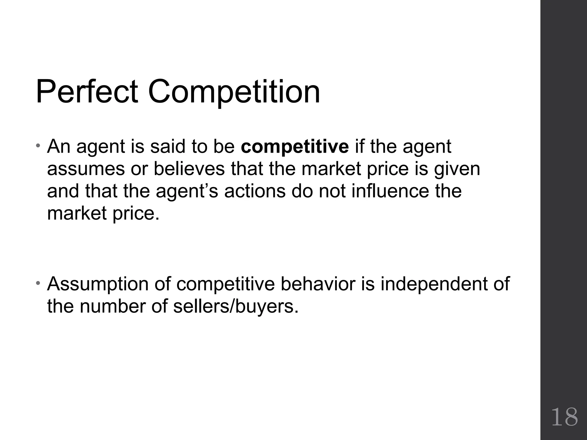
18.
Perfect Competition
• Anagent is said to be competitive if the agent
assumes or believes that the market price is given
and that the agent’s actions do not influence the
market price.
• Assumption of competitive behavior is independent of
the number of sellers/buyers.
18
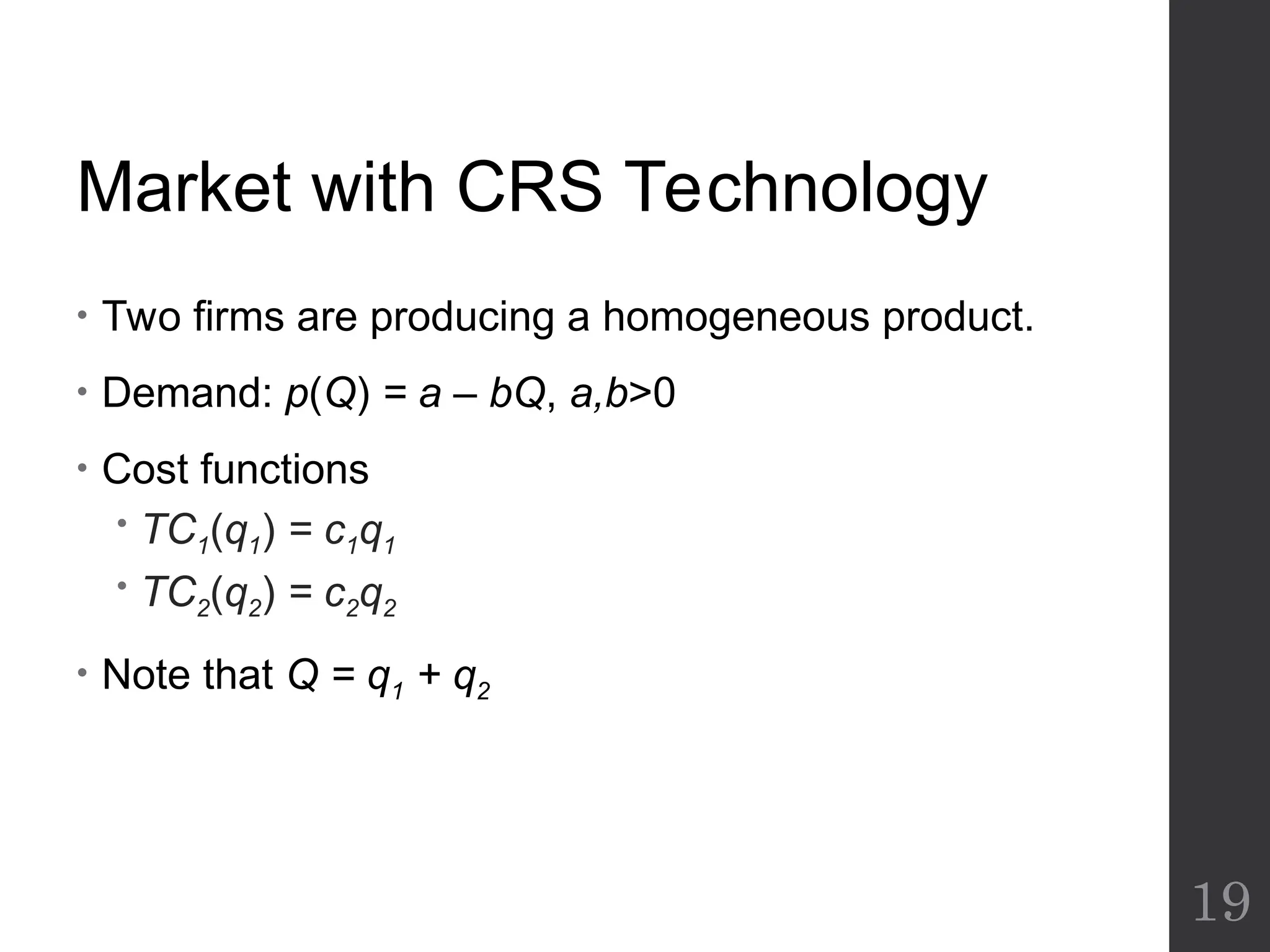
19.
Market with CRSTechnology
• Two firms are producing a homogeneous product.
• Demand: p(Q) = a – bQ, a,b>0
• Cost functions
TC1(q1) = c1q1
TC2(q2) = c2q2
• Note that Q = q1 + q2
19
20.
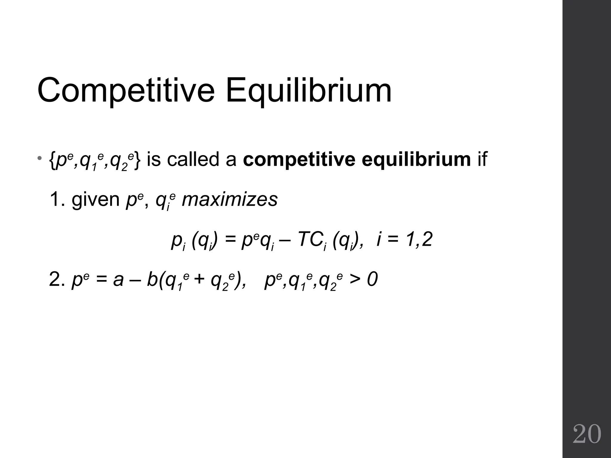
Competitive Equilibrium
• {pe
,q1
e
,q2
e
}is called a competitive equilibrium if
1. given pe
, qi
e
maximizes
pi (qi) = pe
qi – TCi (qi), i = 1,2
2. pe
= a – b(q1
e
+ q2
e
), pe
,q1
e
,q2
e
> 0
20
21.
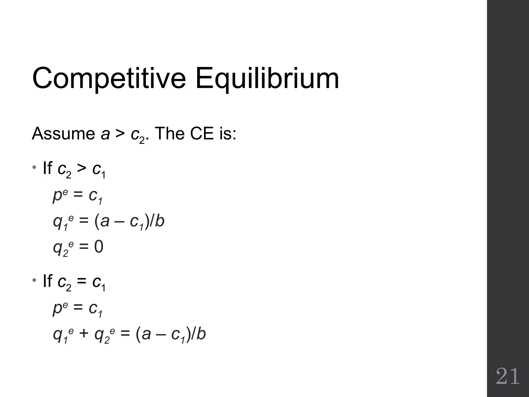
Competitive Equilibrium
Assume a> c2. The CE is:
• If c2 > c1
pe
= c1
q1
e
= (a – c1)/b
q2
e
= 0
• If c2 = c1
pe
= c1
q1
e
+ q2
e
= (a – c1)/b
21
22.
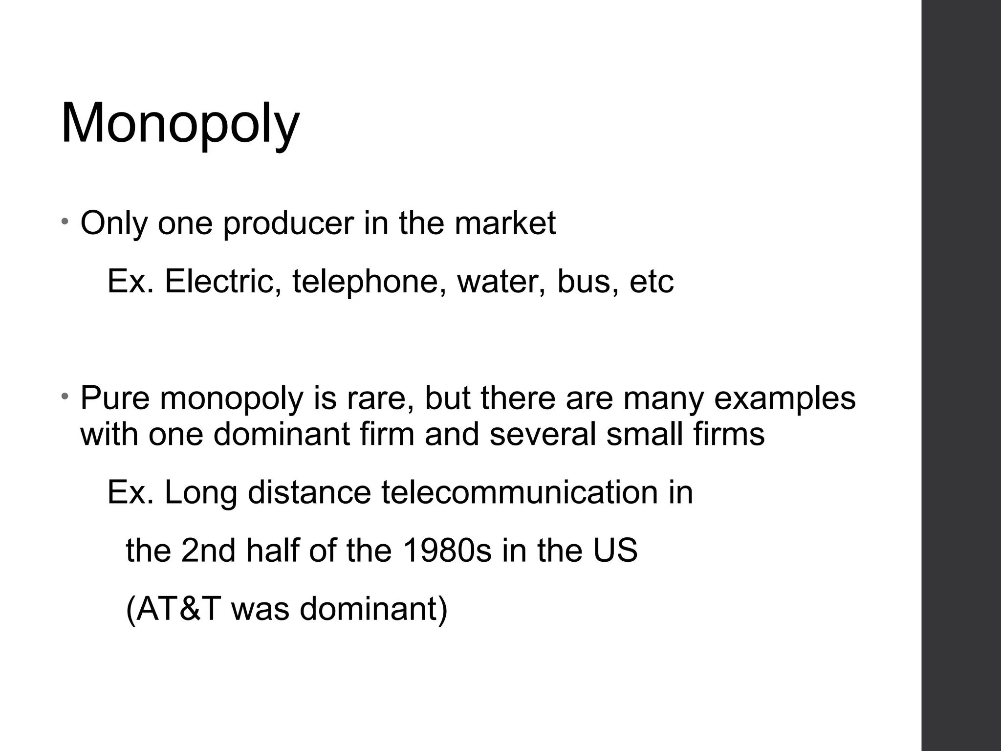
Monopoly
• Only oneproducer in the market
Ex. Electric, telephone, water, bus, etc
• Pure monopoly is rare, but there are many examples
with one dominant firm and several small firms
Ex. Long distance telecommunication in
the 2nd half of the 1980s in the US
(AT&T was dominant)
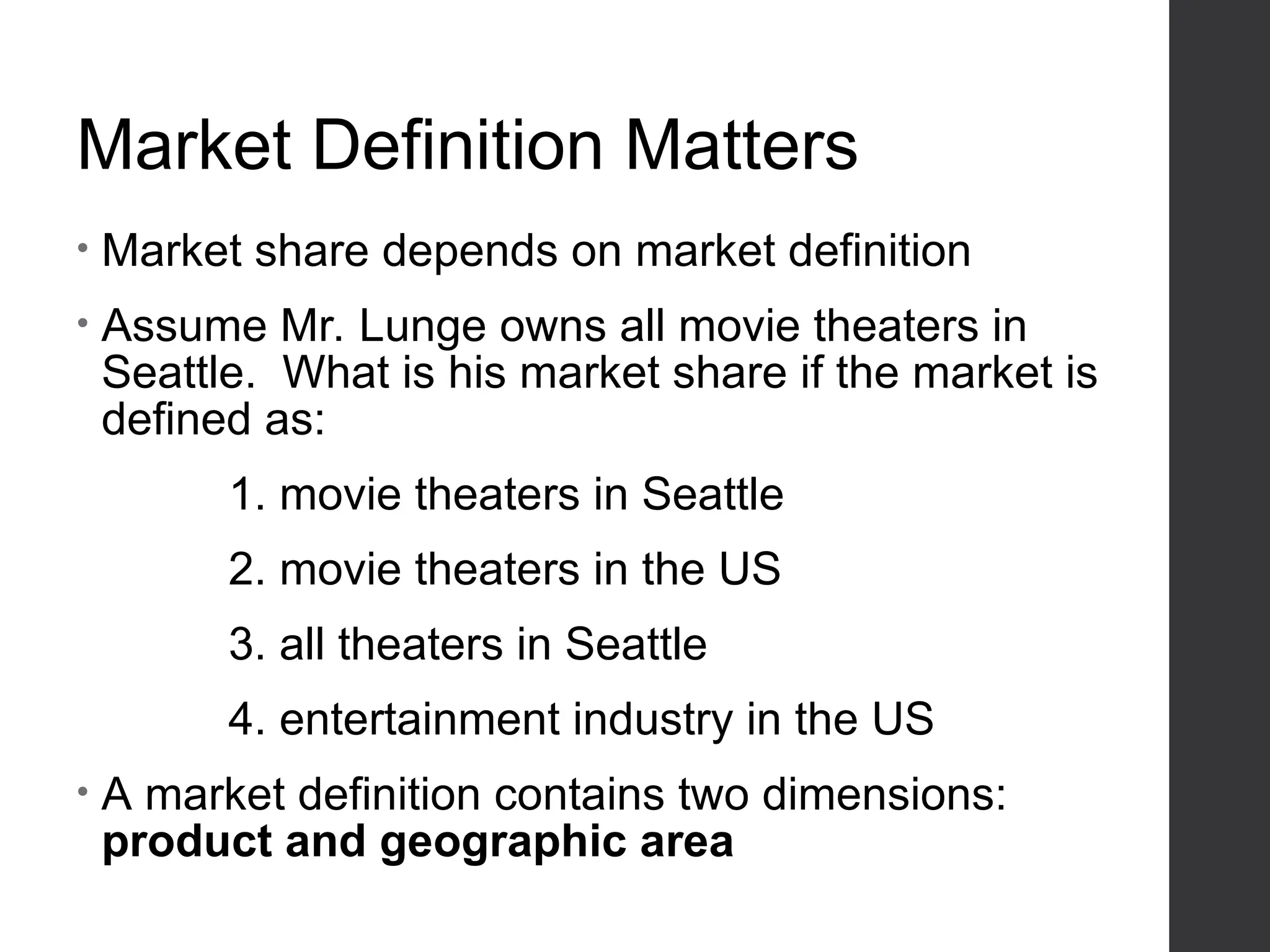
Market Definition Matters
•Market share depends on market definition
• Assume Mr. Lunge owns all movie theaters in
Seattle. What is his market share if the market is
defined as:
1. movie theaters in Seattle
2. movie theaters in the US
3. all theaters in Seattle
4. entertainment industry in the US
• A market definition contains two dimensions:
product and geographic area
25.
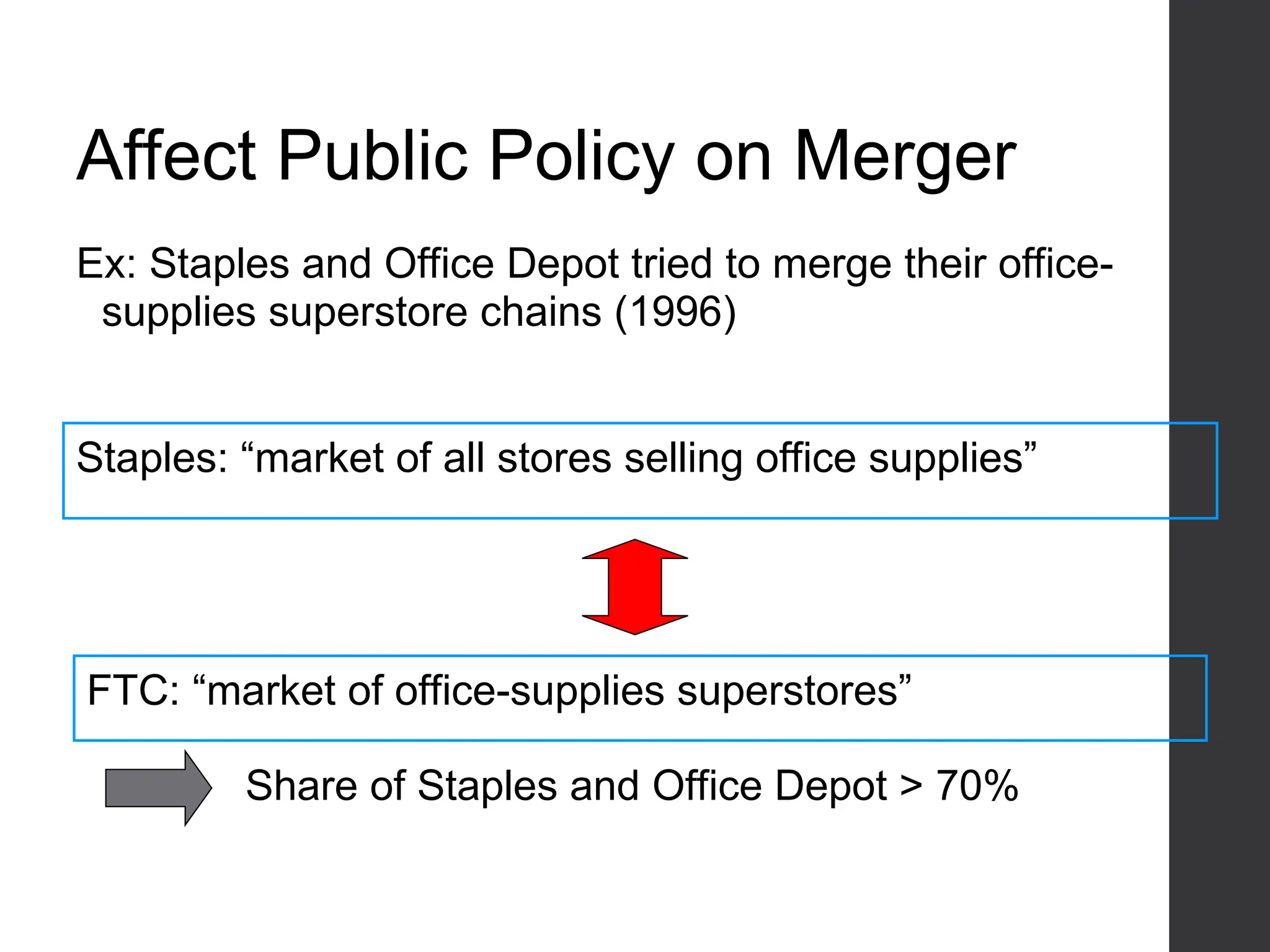
Affect Public Policyon Merger
Ex: Staples and Office Depot tried to merge their office-
supplies superstore chains (1996)
Staples: “market of all stores selling office supplies”
FTC: “market of office-supplies superstores”
Share of Staples and Office Depot > 70%
26.
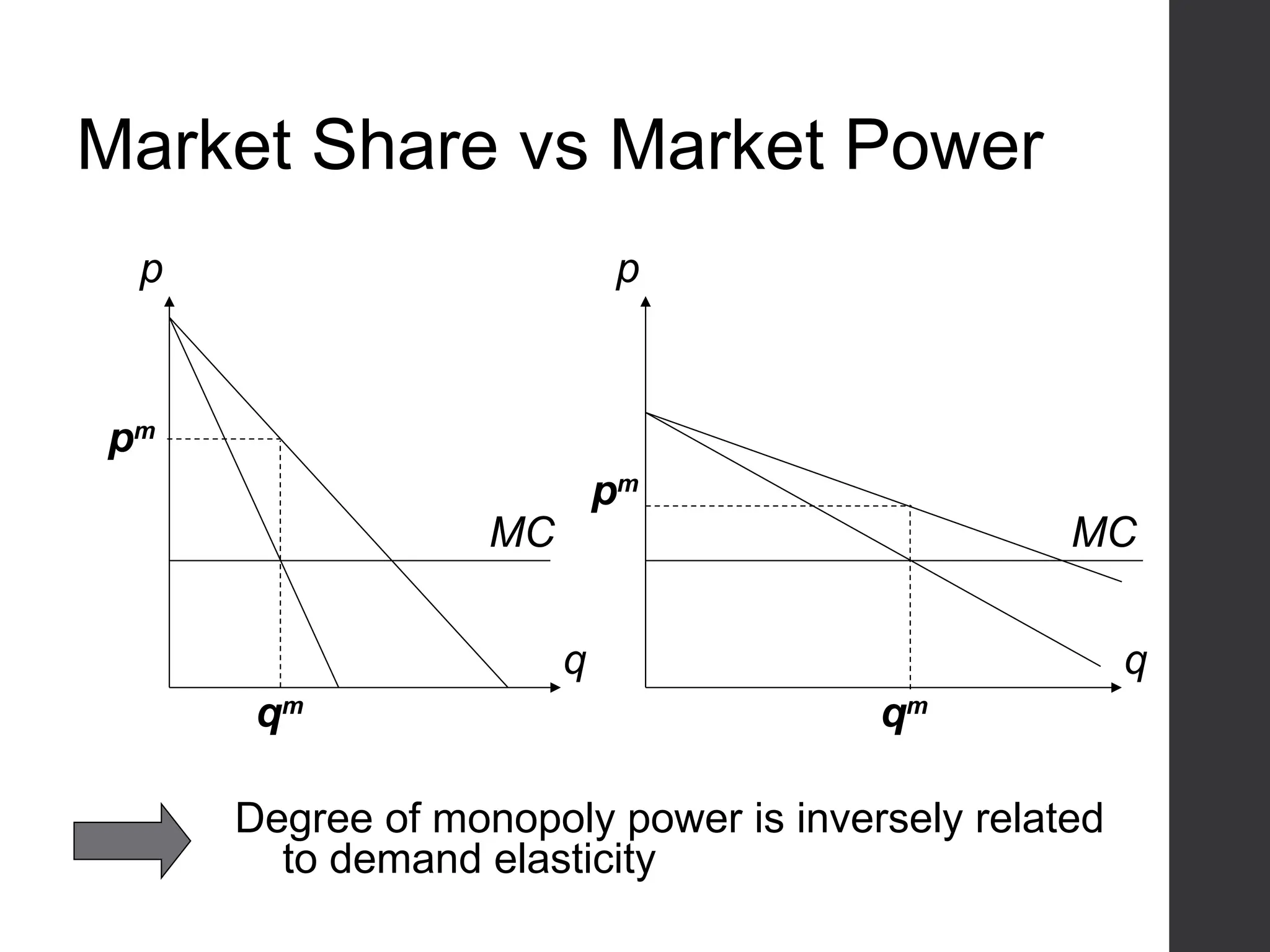
Market Share vsMarket Power
p
p
q q
MC MC
pm
pm
qm
qm
Degree of monopoly power is inversely related
to demand elasticity
27.
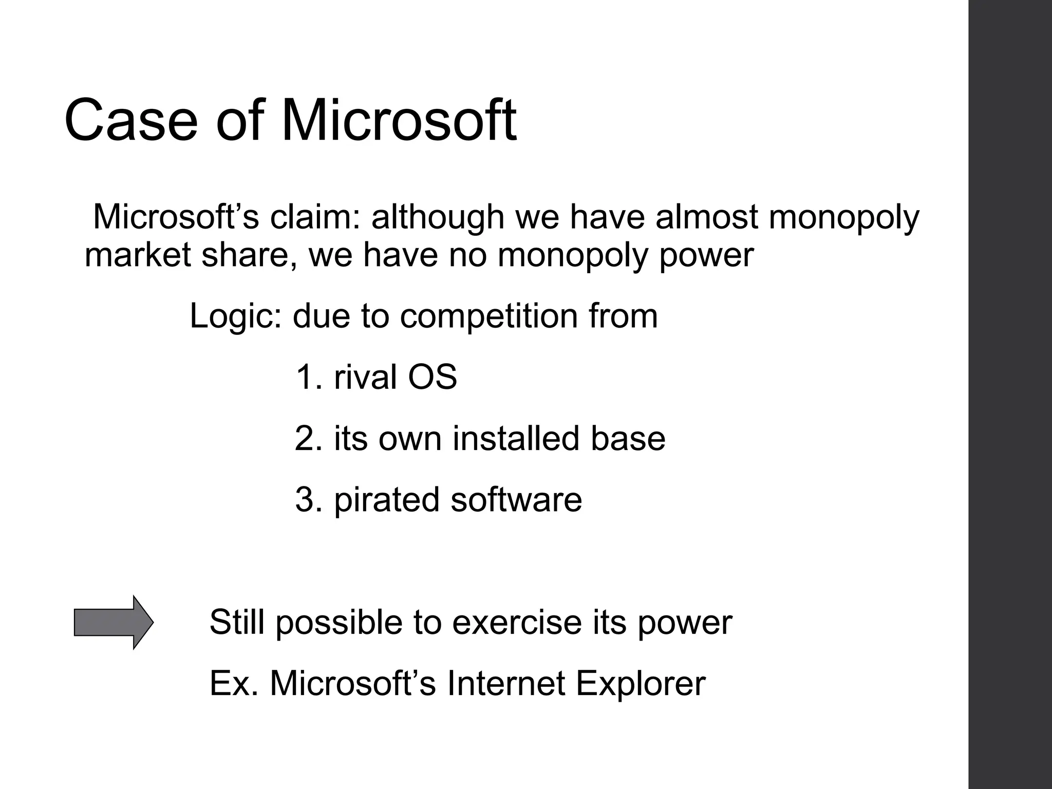
Case of Microsoft
Microsoft’sclaim: although we have almost monopoly
market share, we have no monopoly power
Logic: due to competition from
1. rival OS
2. its own installed base
3. pirated software
Still possible to exercise its power
Ex. Microsoft’s Internet Explorer
28.
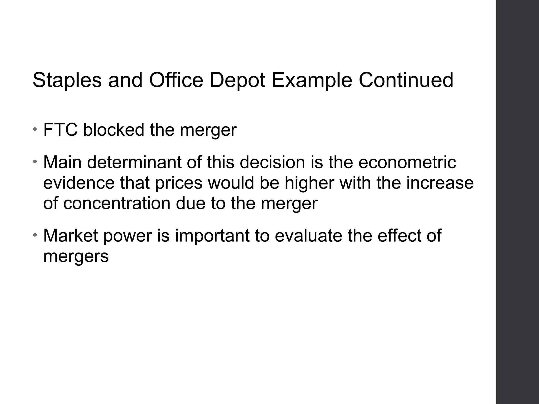
Staples and OfficeDepot Example Continued
• FTC blocked the merger
• Main determinant of this decision is the econometric
evidence that prices would be higher with the increase
of concentration due to the merger
• Market power is important to evaluate the effect of
mergers
29.
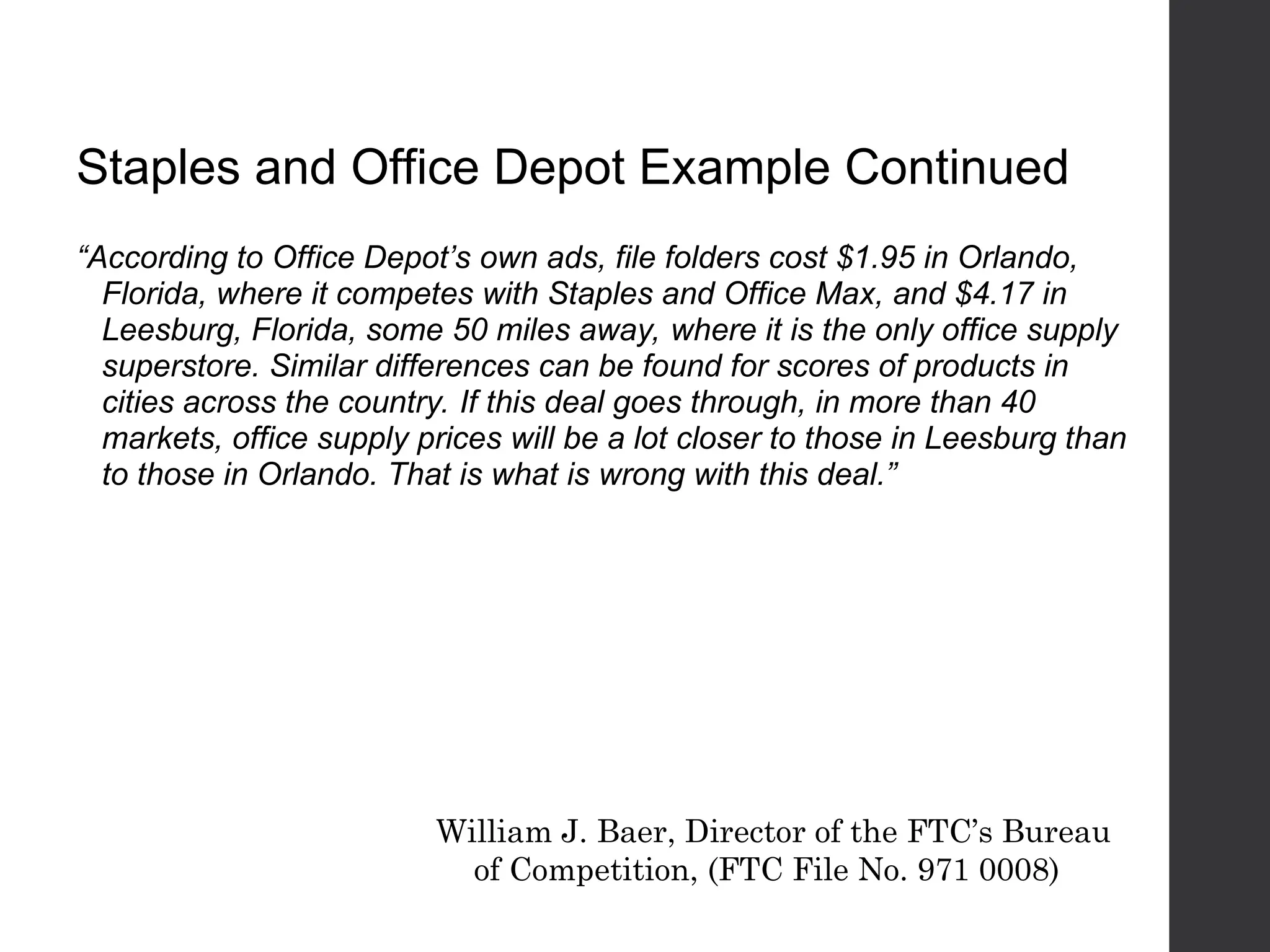
Staples and OfficeDepot Example Continued
“According to Office Depot’s own ads, file folders cost $1.95 in Orlando,
Florida, where it competes with Staples and Office Max, and $4.17 in
Leesburg, Florida, some 50 miles away, where it is the only office supply
superstore. Similar differences can be found for scores of products in
cities across the country. If this deal goes through, in more than 40
markets, office supply prices will be a lot closer to those in Leesburg than
to those in Orlando. That is what is wrong with this deal.”
William J. Baer, Director of the FTC’s Bureau
of Competition, (FTC File No. 971 0008)
30.
Regulation
• Monopoly pricingusually generates inefficiency
• When competition cannot improve efficiency
(e.g., when scale economies are very
important), regulation may achieve the goal.
31.
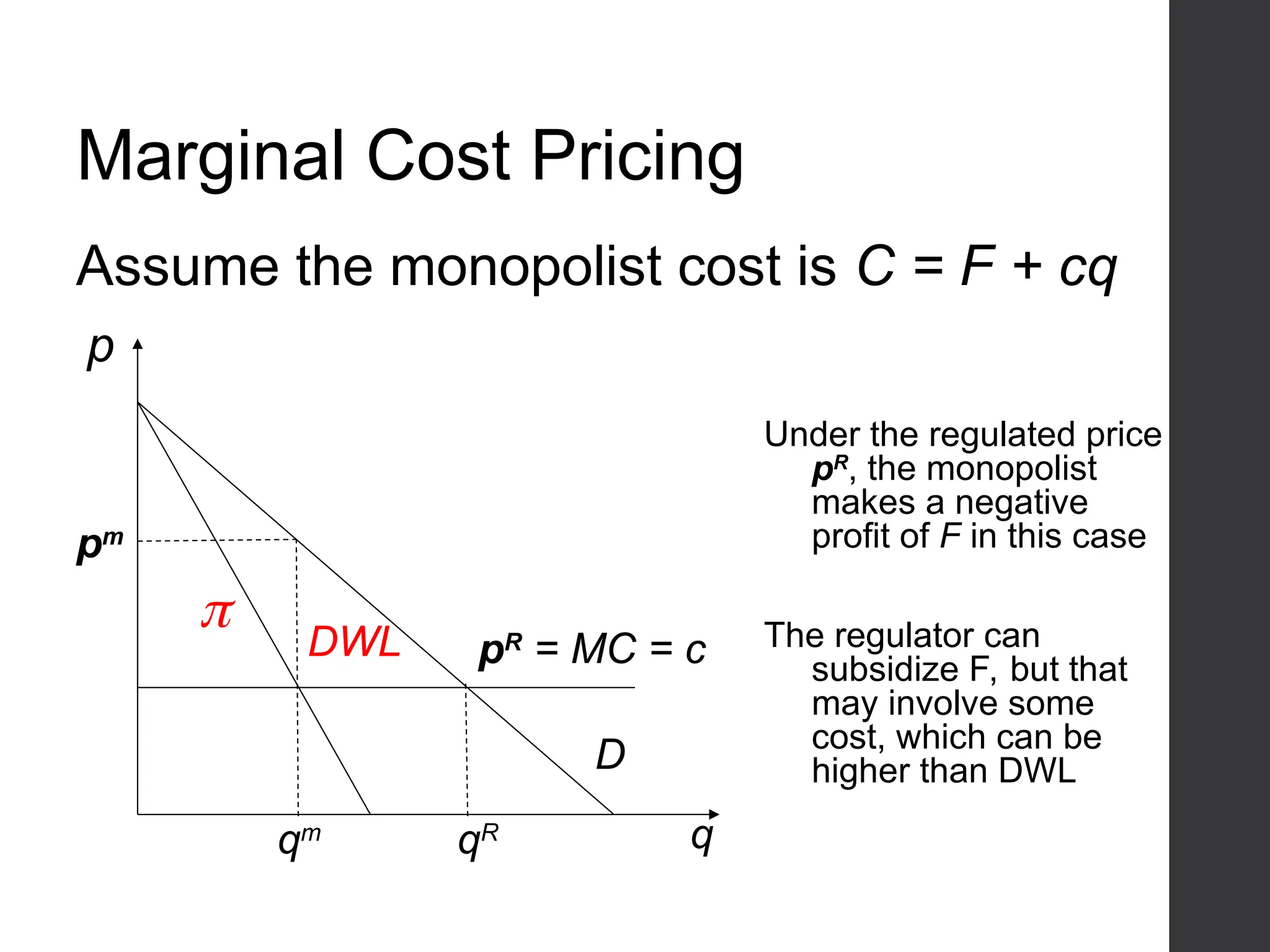
Marginal Cost Pricing
p
qmq
pR
= MC = c
pm
Assume the monopolist cost is C = F + cq
qR
DWL
Under the regulated price
pR
, the monopolist
makes a negative
profit of F in this case
The regulator can
subsidize F, but that
may involve some
cost, which can be
higher than DWL
D
32.
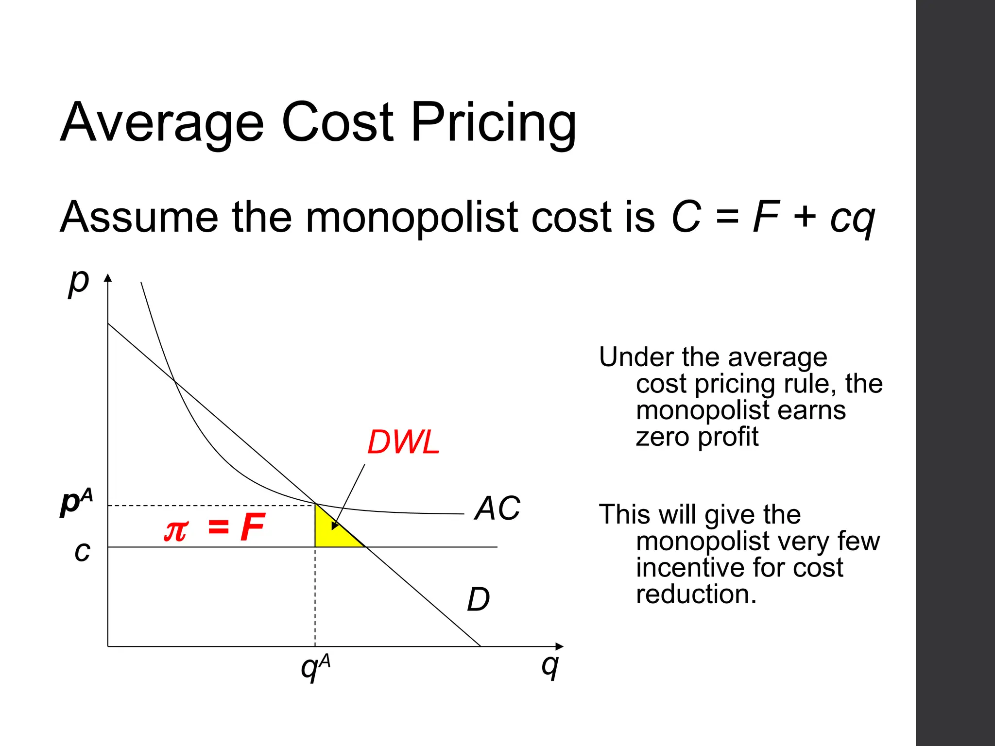
Average Cost Pricing
p
q
AC
pA
Assumethe monopolist cost is C = F + cq
qA
= F
DWL
Under the average
cost pricing rule, the
monopolist earns
zero profit
This will give the
monopolist very few
incentive for cost
reduction.
D
c
33.
Oligopolistic Market
• Amarket with small number of firms
• Called duopoly if there are only two firms
• Take other firms’ actions into account
• Two commonly used model
Firms simultaneously choose quantity (Cournot)
Firms simultaneously choose price (Bertrand)
33
34.
Cournot Market Structure
•Firms choose quantity simultaneously
• There are several variants:
Homogeneous or differentiated products
One-shot or repeated interaction
Sequential moves
• Now we assume
Firms sell homogeneous products
Demand is given by p(Q) = a – b(Q)
Cost function given by TC(q) = cq, c > 0
There are two firms
34
35.
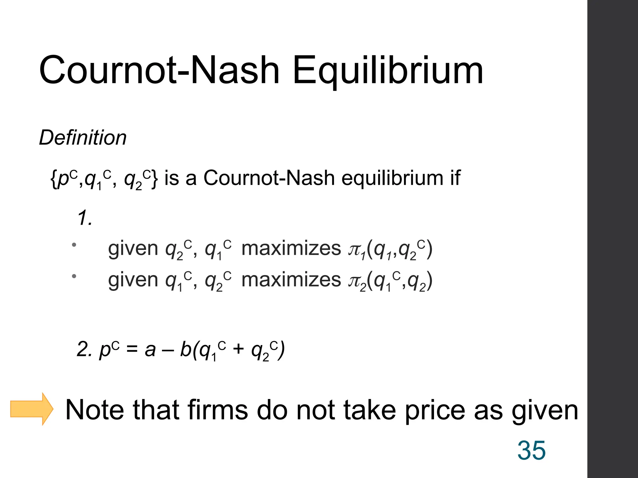
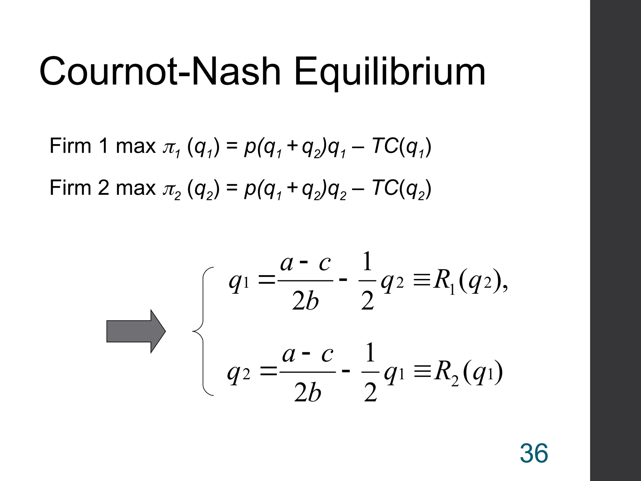
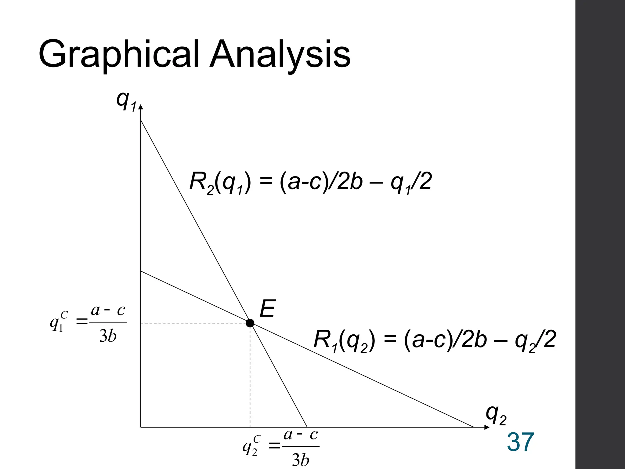
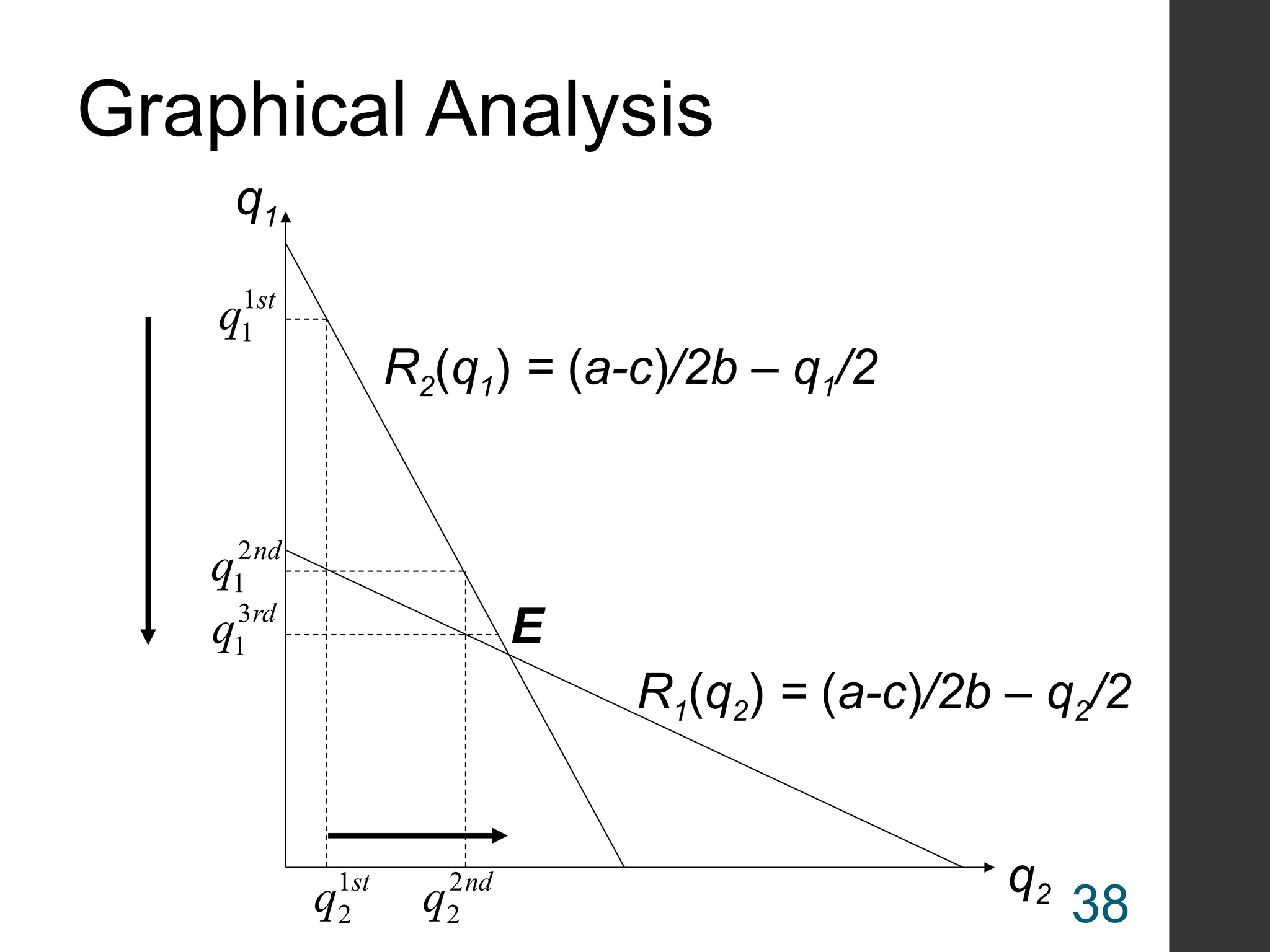
Cournot-Nash Equilibrium
Definition
{pC
,q1
C
, q2
C
}is a Cournot-Nash equilibrium if
1.
given q2
C
, q1
C
maximizes 1(q1,q2
C
)
given q1
C
, q2
C
maximizes 2(q1
C
,q2)
2. pC
= a – b(q1
C
+ q2
C
)
Note that firms do not take price as given
35
36.
Cournot-Nash Equilibrium
Firm 1max 1 (q1) = p(q1 + q2)q1 – TC(q1)
Firm 2 max 2 (q2) = p(q1 + q2)q2 – TC(q2)
),
(
2
1
2
2
1
2
1 q
R
q
b
c
a
q
)
(
2
1
2
1
2
1
2 q
R
q
b
c
a
q
36
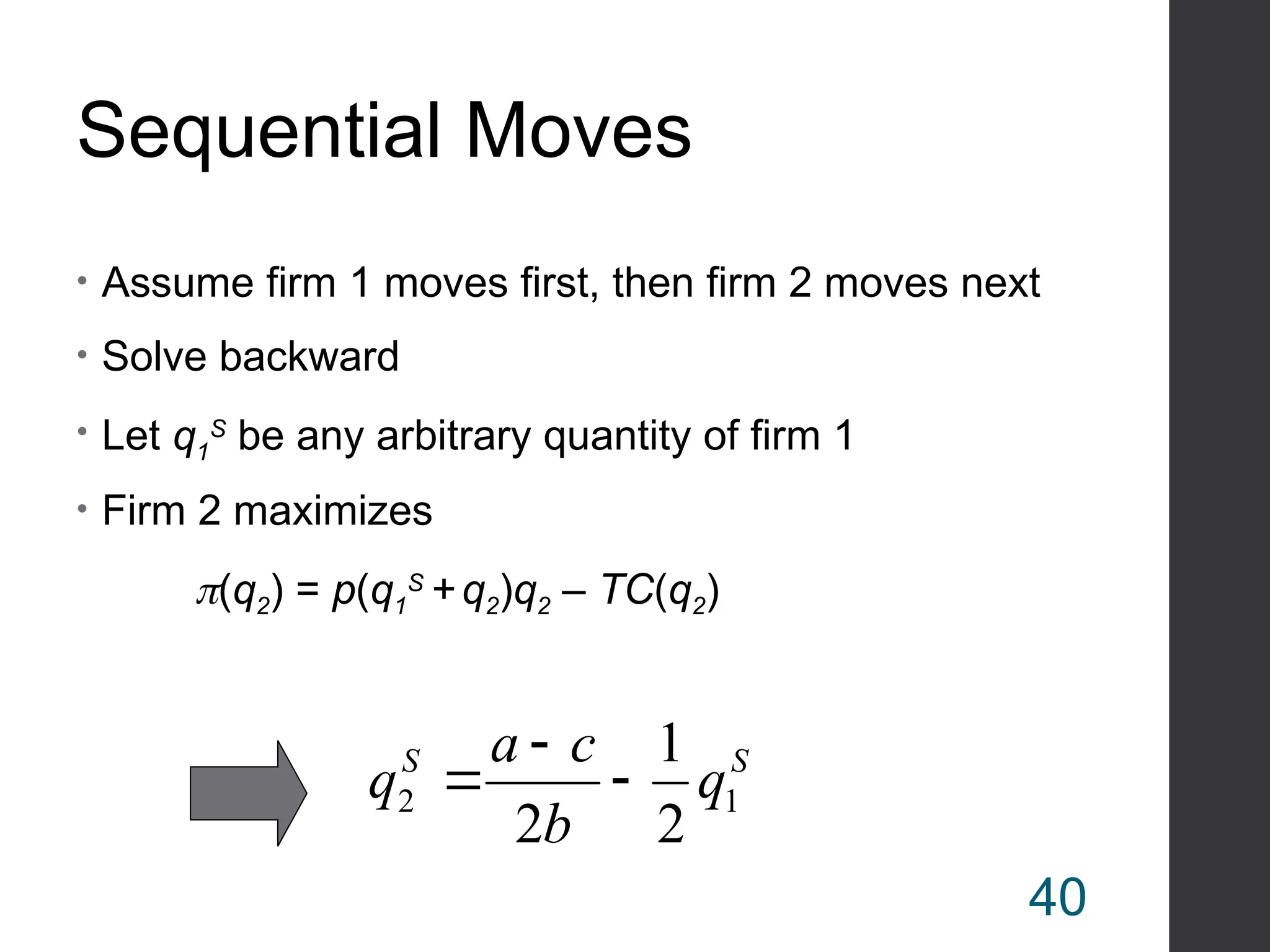
Sequential Moves
• Assumefirm 1 moves first, then firm 2 moves next
• Solve backward
• Let q1
S
be any arbitrary quantity of firm 1
• Firm 2 maximizes
(q2) = p(q1
S
+ q2)q2 – TC(q2)
S
S
q
b
c
a
q 1
2
2
1
2
40
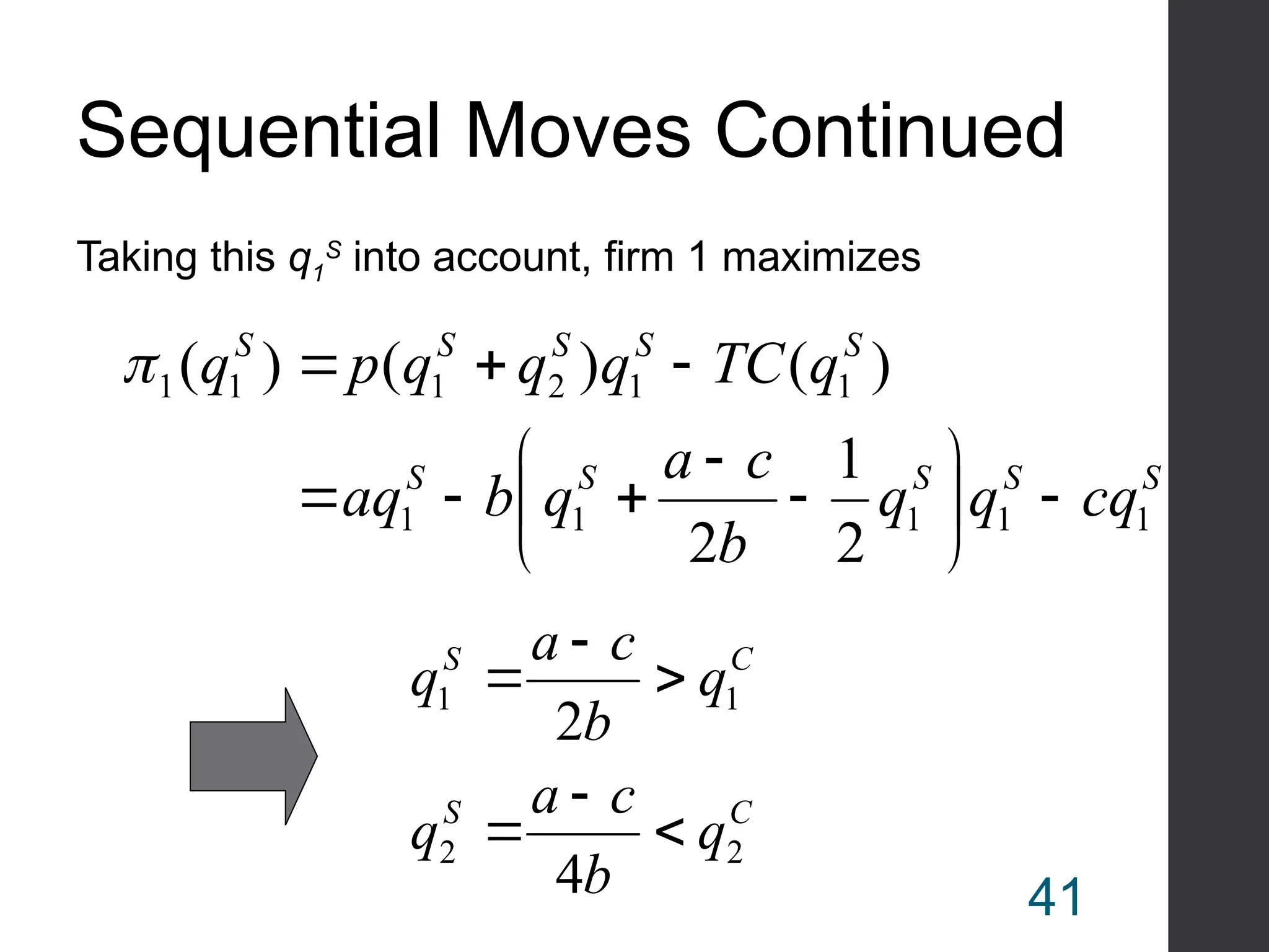
41.
Sequential Moves Continued
Takingthis q1
S
into account, firm 1 maximizes
S
S
S
S
S
S
S
S
S
S
cq
q
q
b
c
a
q
b
aq
q
TC
q
q
q
p
q
1
1
1
1
1
1
1
2
1
1
1
2
1
2
)
(
)
(
)
(
C
S
C
S
q
b
c
a
q
q
b
c
a
q
2
2
1
1
4
2
41
42.
Bertrand Market Structure
•Firms choose price simultaneously
• There are several variants:
Homogeneous or differentiated products
One-shot or repeated interaction
Sequential moves
• Now we assume the same set of assumptions as in the
analysis of the Cournot model
42
43.
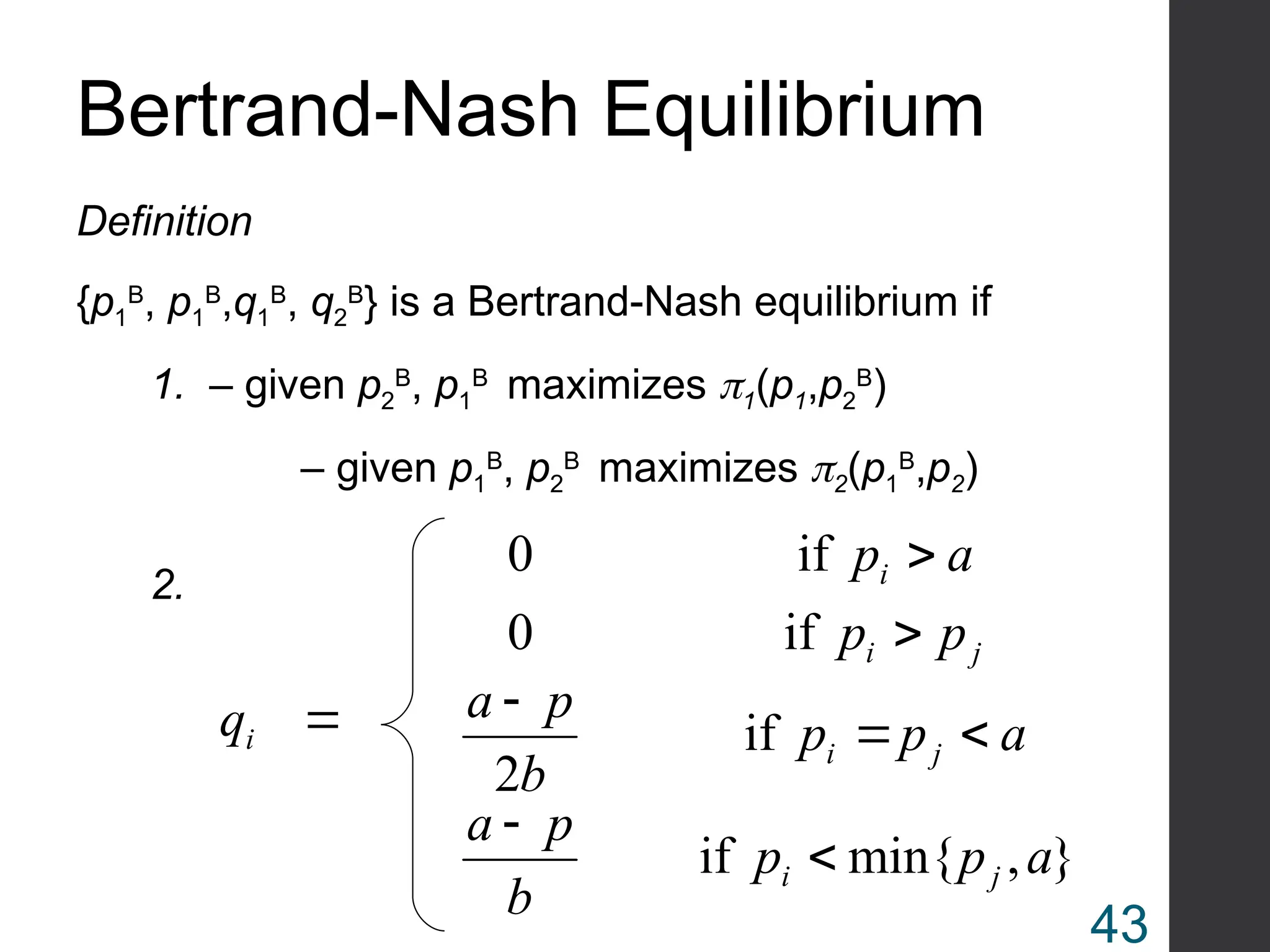
Bertrand-Nash Equilibrium
Definition
{p1
B
, p1
B
,q1
B
,q2
B
} is a Bertrand-Nash equilibrium if
1. – given p2
B
, p1
B
maximizes 1(p1,p2
B
)
– given p1
B
, p2
B
maximizes 2(p1
B
,p2)
}
,
min{
if
if
2
if
0
if
0
a
p
p
b
p
a
a
p
p
b
p
a
p
p
a
p
q
j
i
j
i
j
i
i
i
2.
43
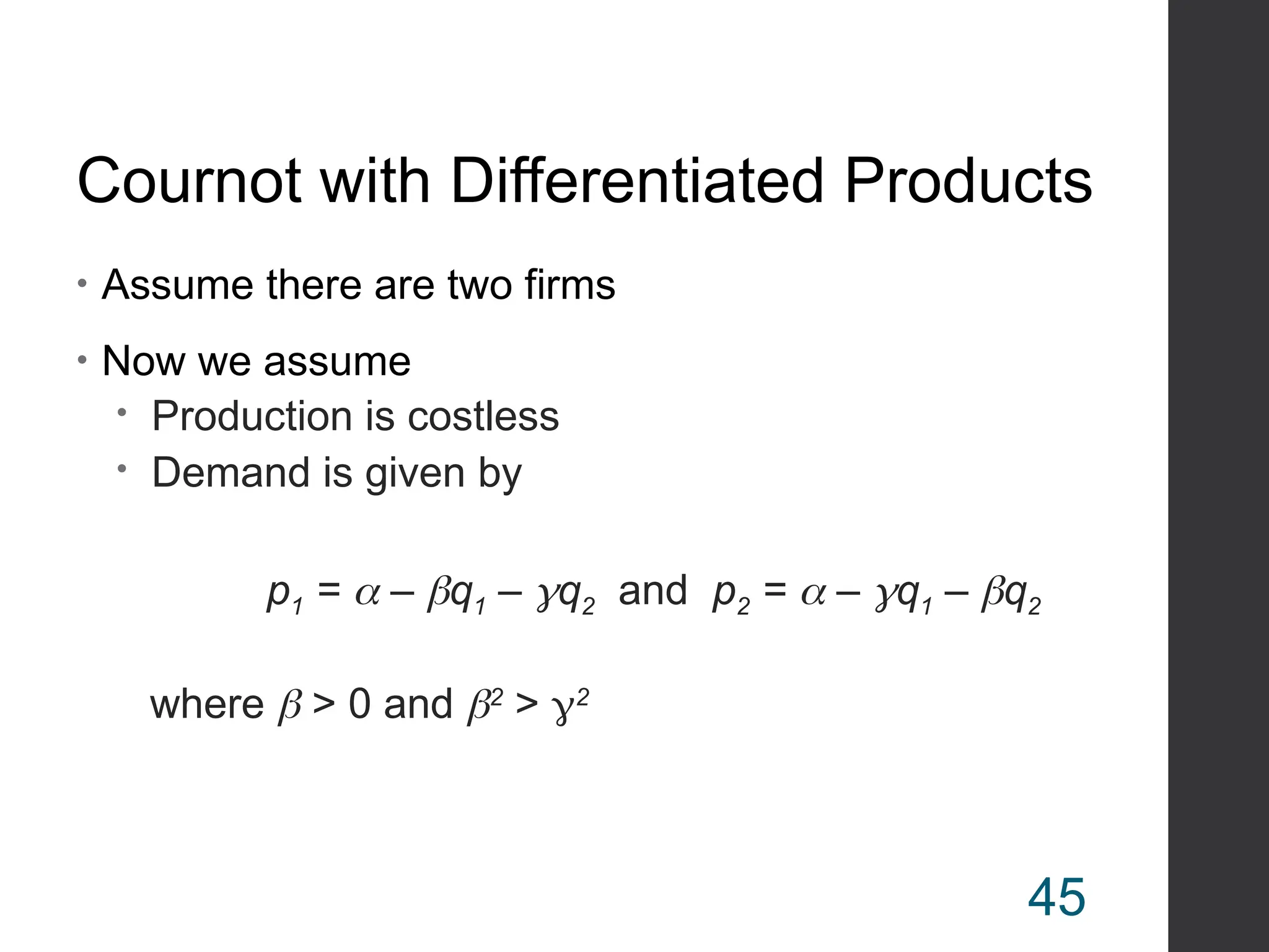
Cournot with DifferentiatedProducts
• Assume there are two firms
• Now we assume
Production is costless
Demand is given by
p1 = – q1 – q2 and p2 = – q1 – q2
where > 0 and 2
> 2
45
46.
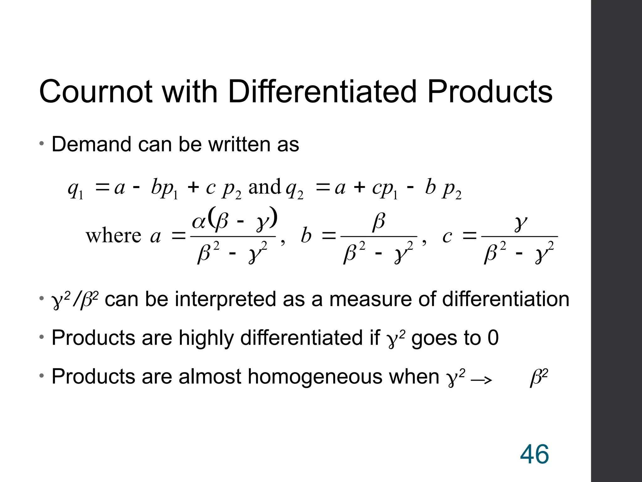
Cournot with DifferentiatedProducts
• Demand can be written as
• 2
/2
can be interpreted as a measure of differentiation
• Products are highly differentiated if 2
goes to 0
• Products are almost homogeneous when 2
2
2
2
2
2
2
2
2
1
2
2
1
1
,
,
where
and
c
b
a
p
b
cp
a
q
p
c
bp
a
q
46
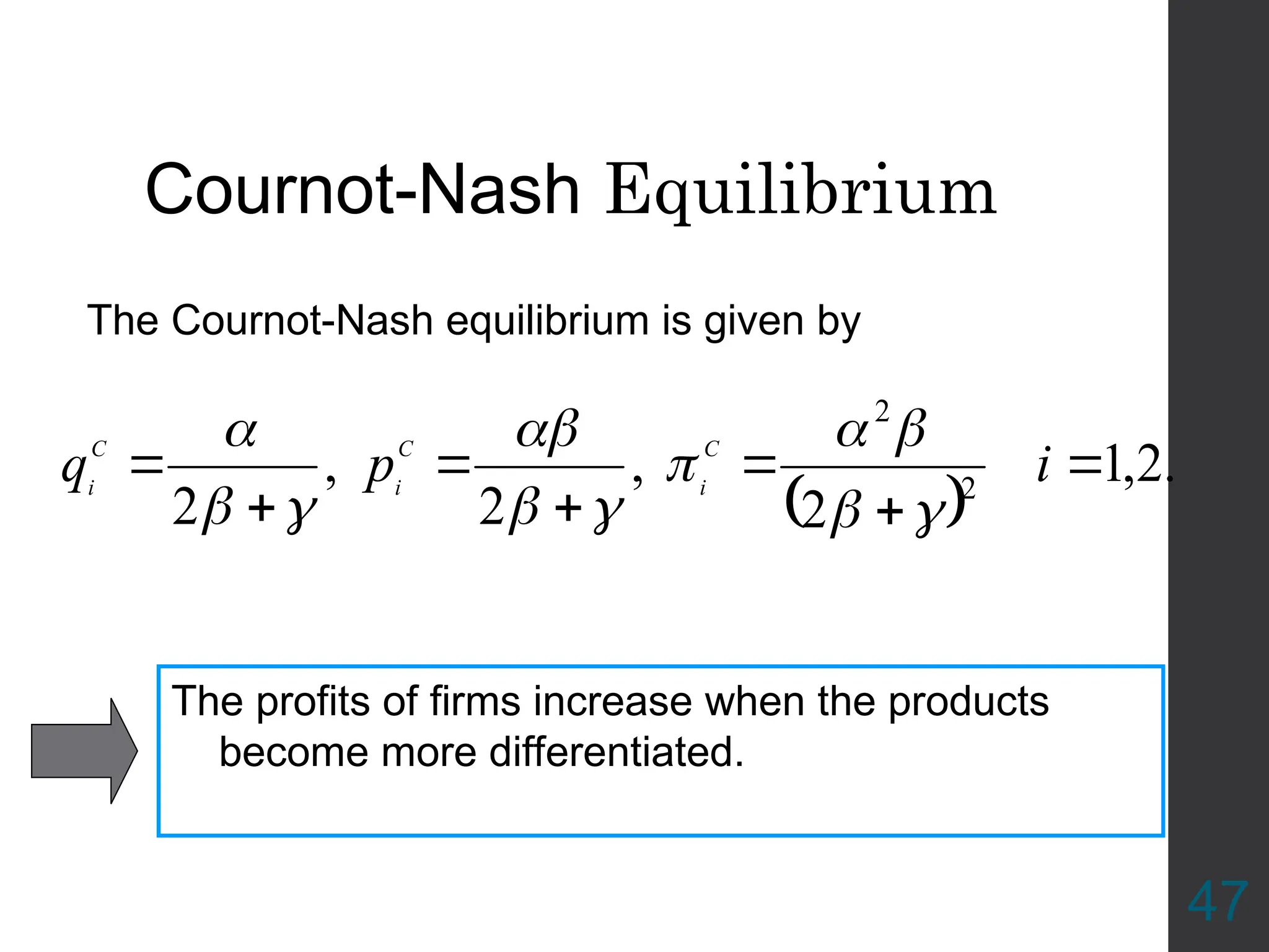
47.
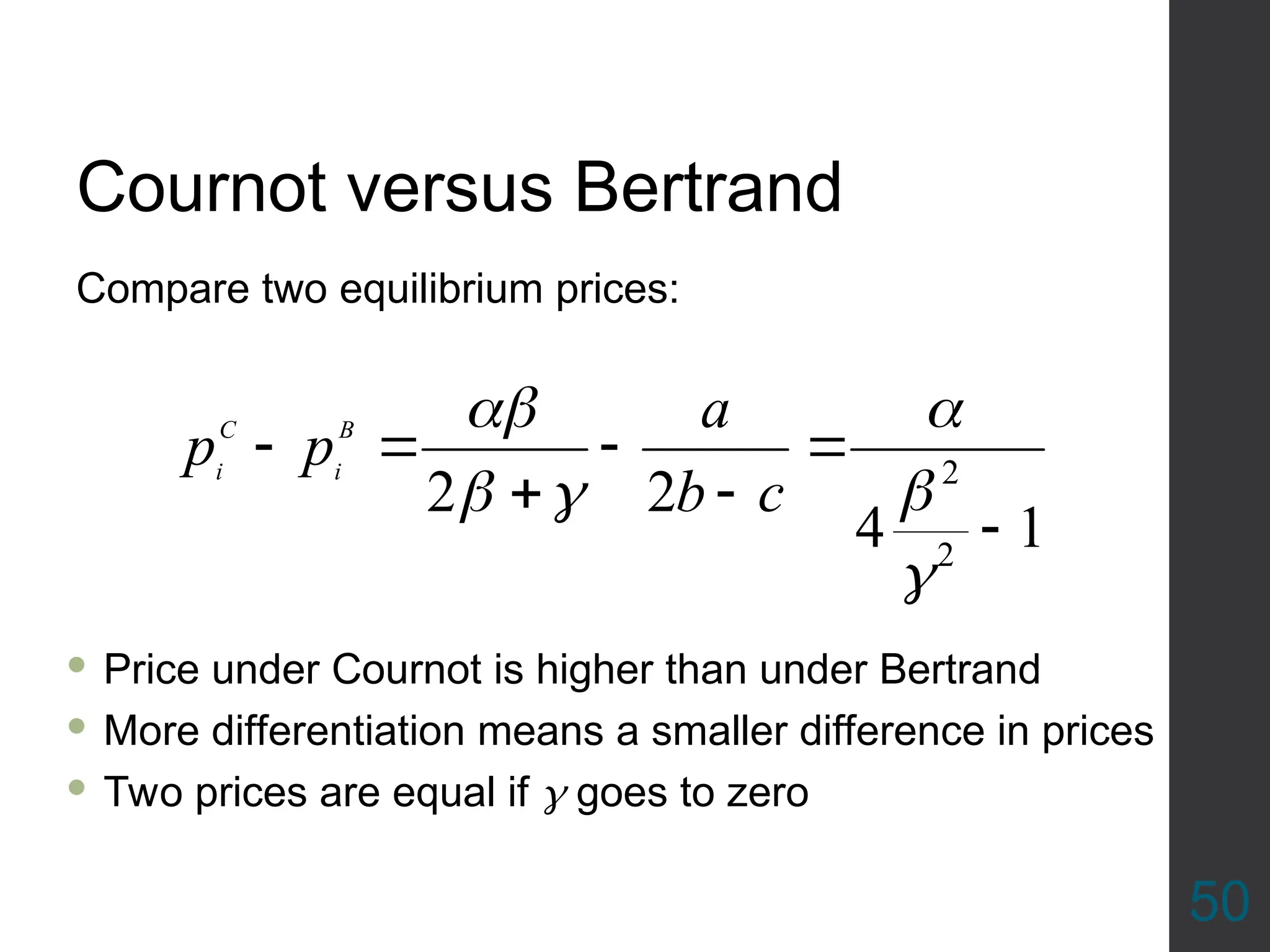
Cournot-Nash Equilibrium
.
2
,
1
2
,
2
,
22
2
i
p
q C
i
C
i
C
i
The profits of firms increase when the products
become more differentiated.
The Cournot-Nash equilibrium is given by
47
48.
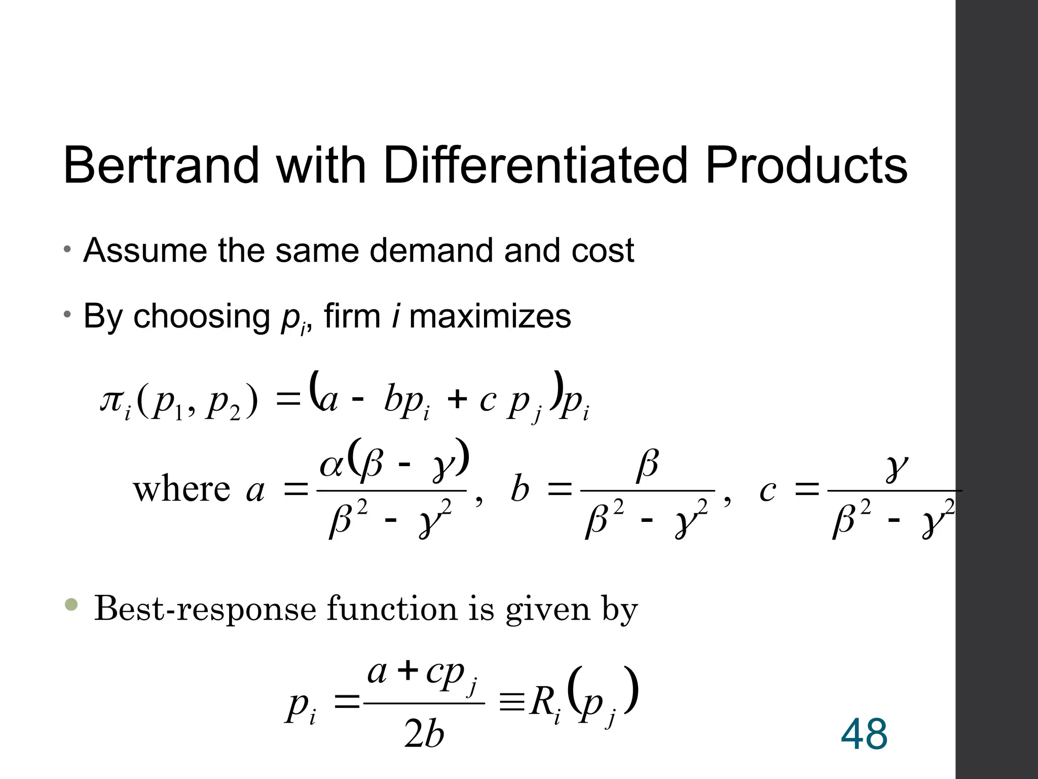
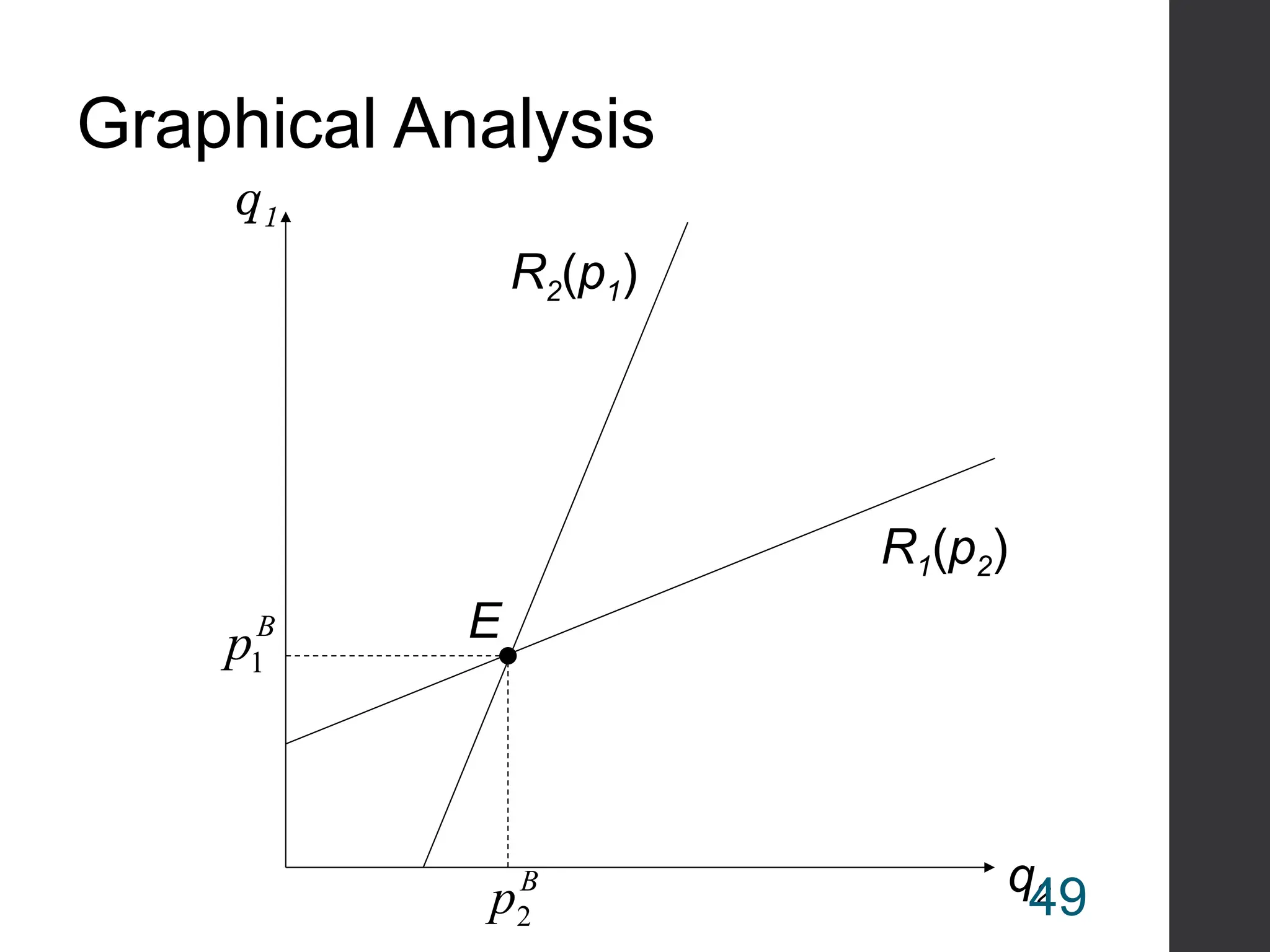
Bertrand with DifferentiatedProducts
• Assume the same demand and cost
• By choosing pi, firm i maximizes
2
2
2
2
2
2
2
1
,
,
where
)
,
(
c
b
a
p
p
c
bp
a
p
p i
j
i
i
j
i
j
i p
R
b
cp
a
p
2
Best-response function is given by
48