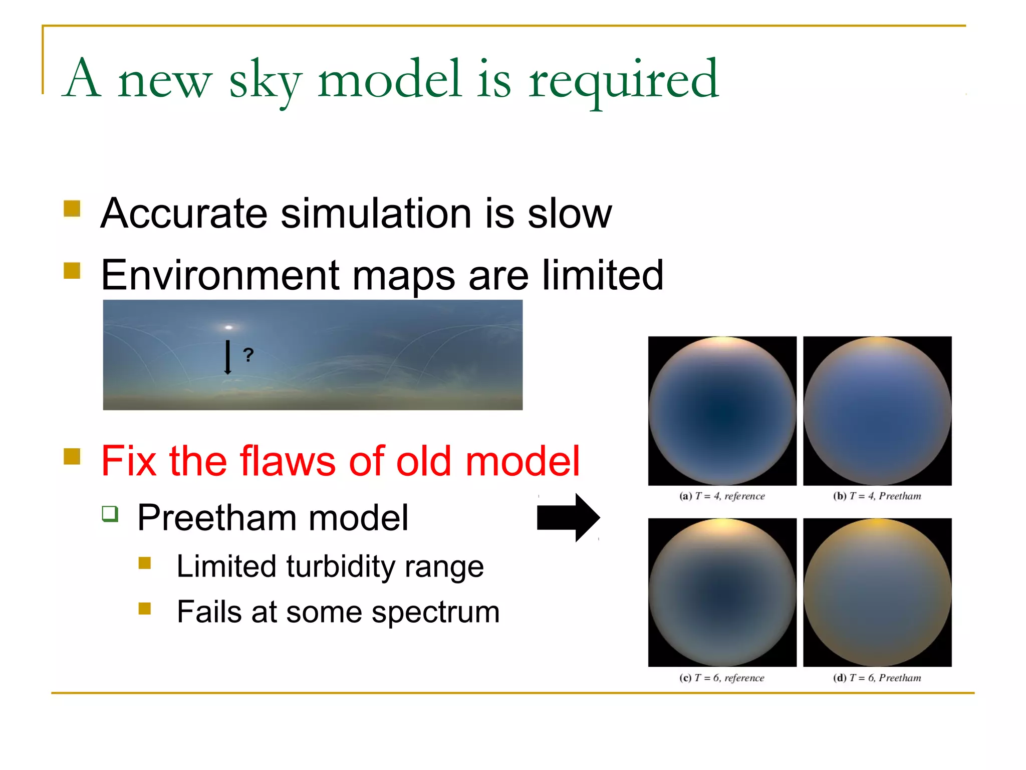
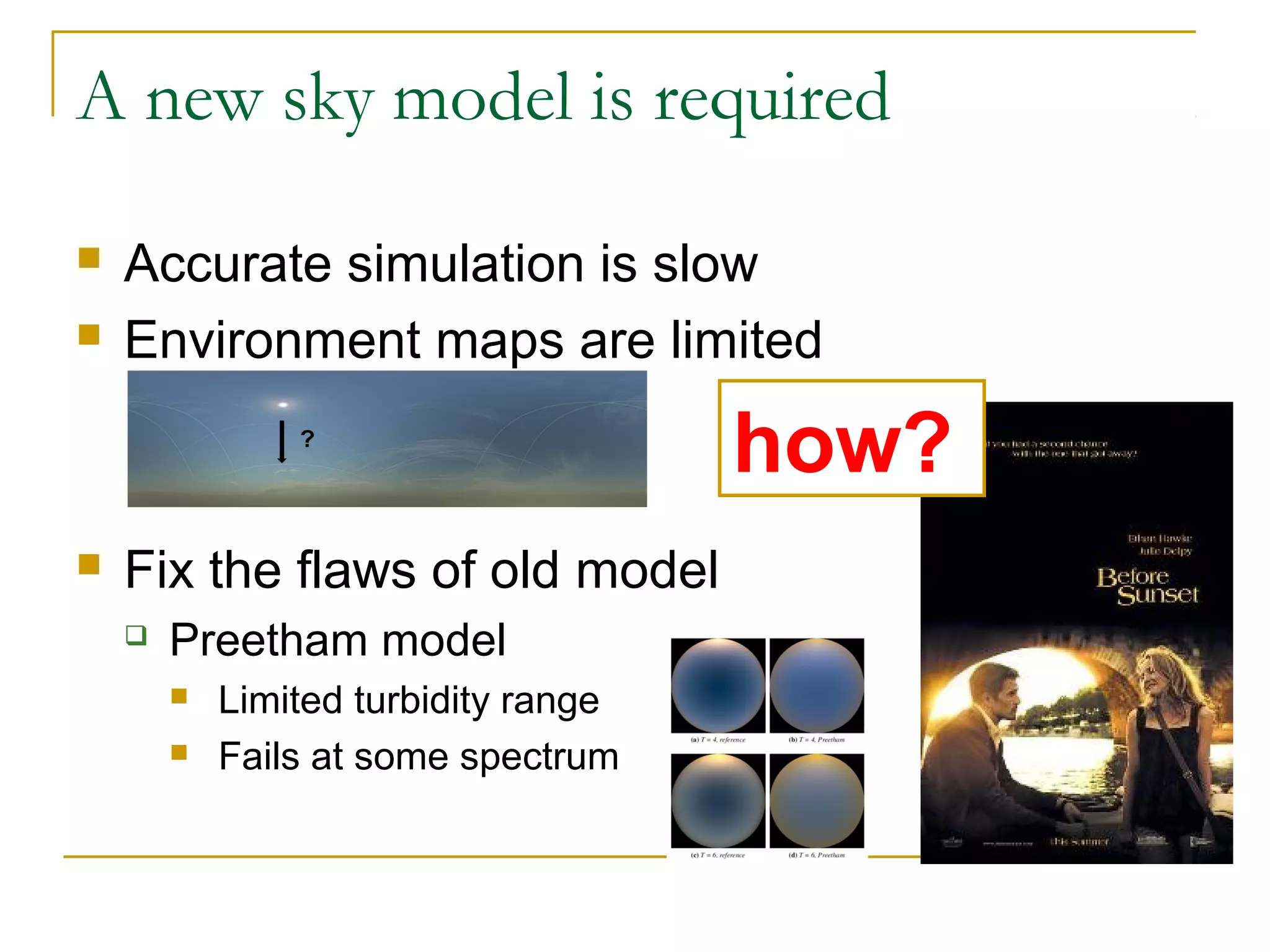
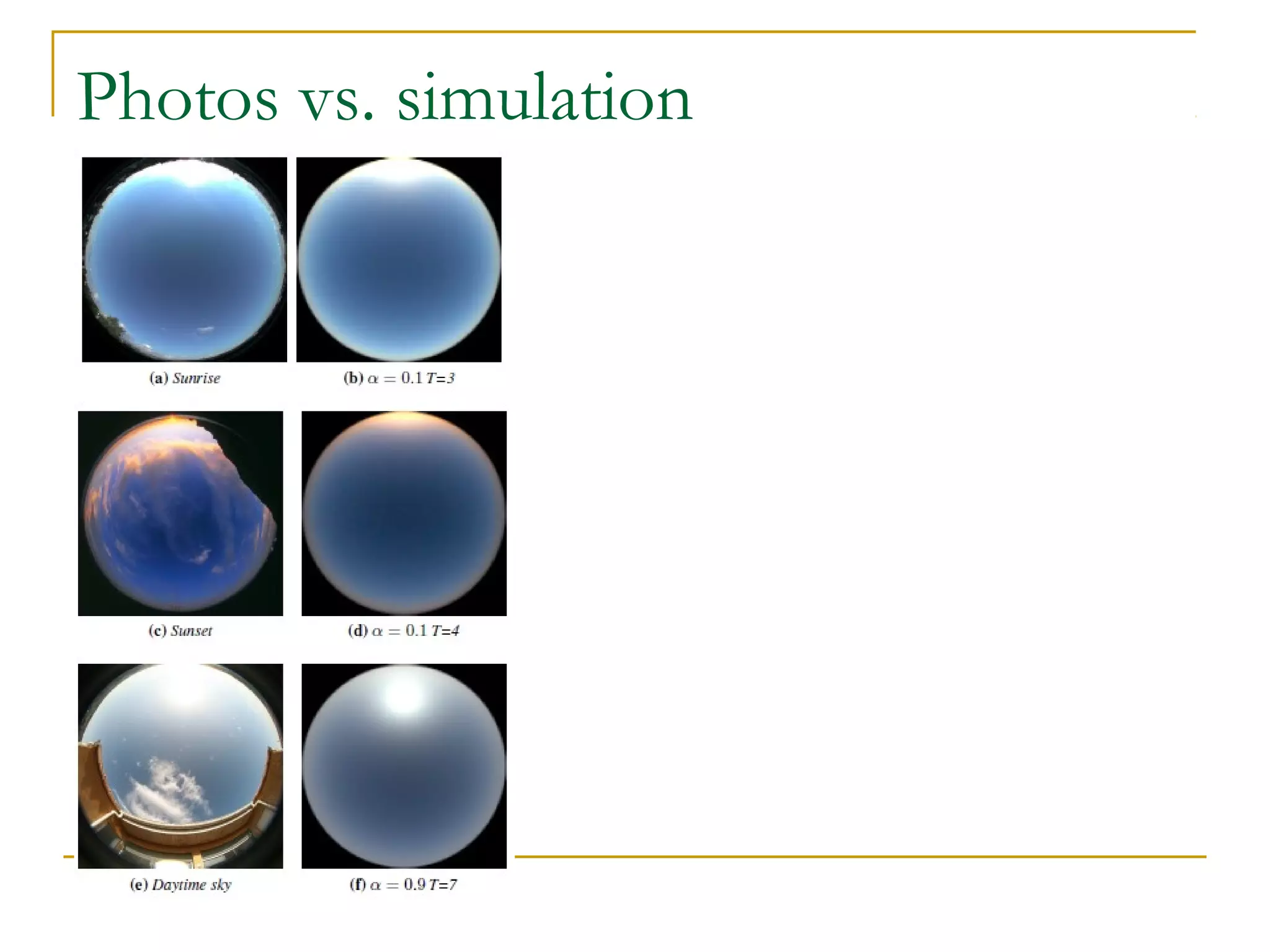
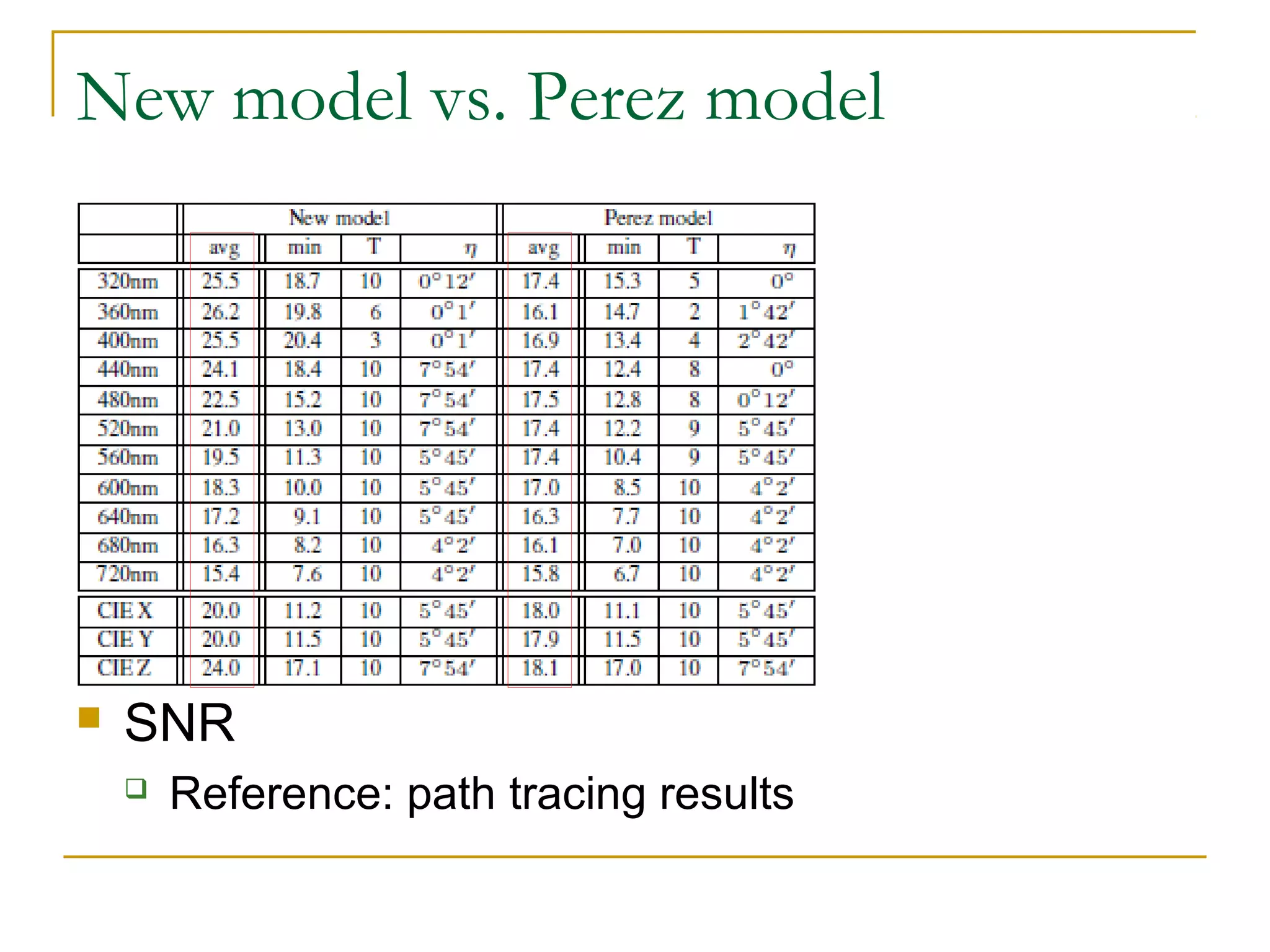
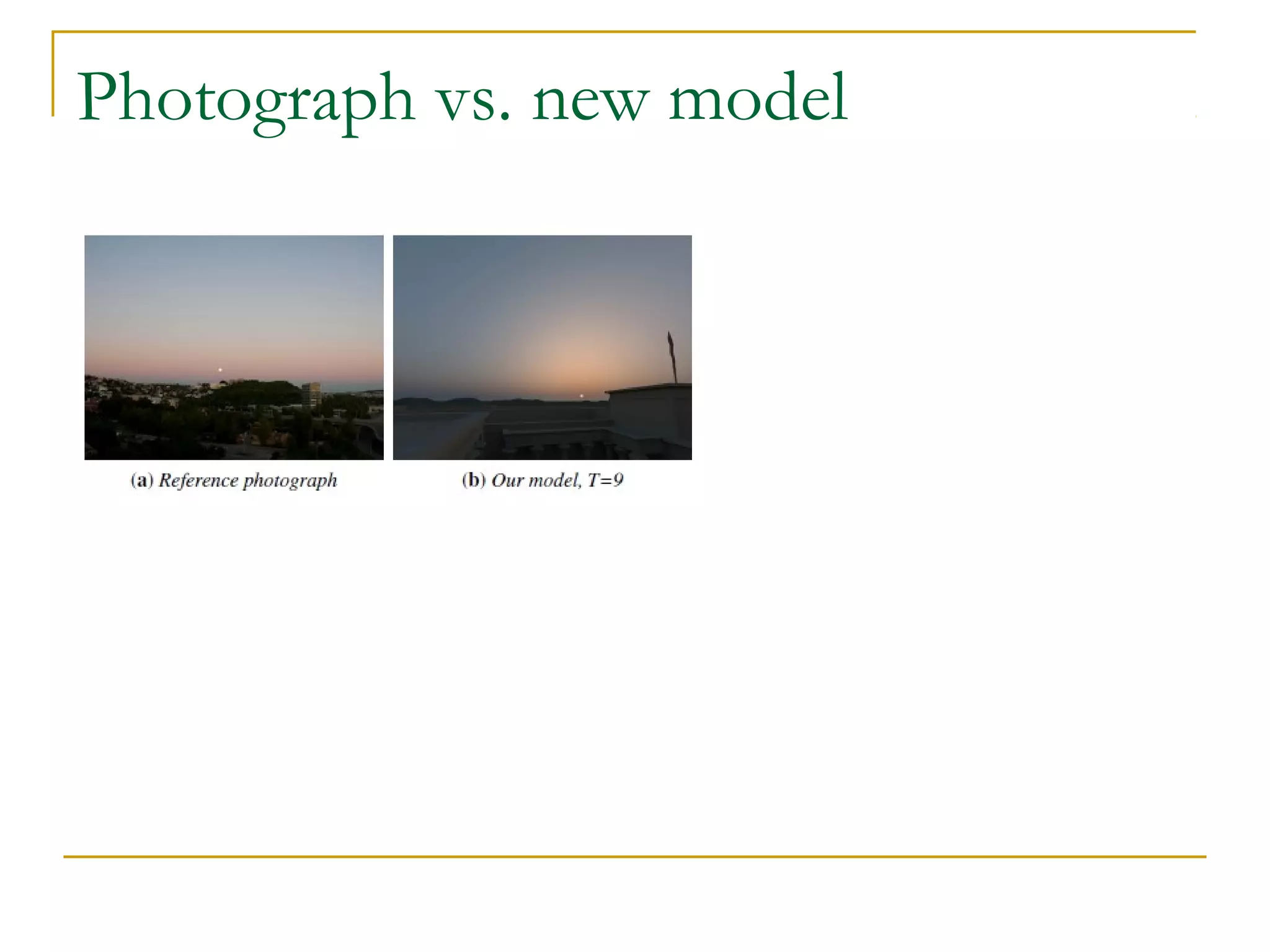
An Analytic Model for
Full Spectral Sky-Dome Radiance
                      SIGRAPH 2012

     2012/12/05
     ked
Authors

   Lukas Hosek, Alexander Wilkie
Outline

   Goal
   Why is the sky blue?
   Modeling
   Simulation
   Results
Outline

   Goal
   Why is the sky blue?
   Modeling
   Simulation
   Results
A new sky model is required

   Accurate simulation is slow
   Environment maps are limited
   Fix the flaws of old model
A new sky model is required

   Accurate simulation is slow
   Environment maps are limited


   Fix the flaws of old model
A new sky model is required

   Accurate simulation is slow
   Environment maps are limited


                   ?


   Fix the flaws of old model
A new sky model is required

   Accurate simulation is slow
   Environment maps are limited


   Fix the flaws of old model
       Preetham model
           Limited turbidity range
           Fails at some spectrum
A new sky model is required

   Accurate simulation is slow
   Environment maps are limited


   Fix the flaws of old model
       Preetham model
           Limited turbidity range
           Fails at some spectrum
A new sky model is required

   Demo
A new sky model is required

   Accurate simulation is slow
   Environment maps are limited

                                      how?
   Fix the flaws of old model
       Preetham model
           Limited turbidity range
           Fails at some spectrum
Outline

   Goal
   Why is the sky blue?
   Modeling
   Simulation
   Results
Scattering
http://www.sciencemadesimple.com/sky_blue.html
Scattering
http://www.sciencemadesimple.com/sky_blue.html


   Effected by
       Haze: dust particles, water droplets, …. (1859)
       Air molecules (1899)
       And finally settle by Einstein (1910)
     “ 方勵之—天空為什麼是藍色
     的”
Scattering – the sky near the horizen
http://www.sciencemadesimple.com/sky_blue.html


                                                 http://www.research-in-germany.de/25326/german-countryside-
                                                 bildergalerie,templateId=popup,currentContentId=25294.html
The red sunset
http://www.sciencemadesimple.com/sky_blue.html


                                                 http://math.ucr.edu/home/baez/physics/General/BlueSky/blue_sky.htm
                                                 l
Outline

   Goal
   Why is the sky blue?
   Modeling
   Simulation
   Results
Luminance model

   Perez (1993)



       The parameters A to E and Yz are used to tune
        the luminance distribution.
Spectral radiance model

   Preetham (1999)






                      CIE xyY color space
Spectral radiance model

   Preetham (1999)
   The parameters of Perez model (A to E and
    Yz) are linear functions of condition, turbidity.
   Turbidity,
       Ratio of the optical thickness to pure air
           T=2: very clear, Arctic-like sky
           T=3: clear sky in temperate climate
           T=6: warm, moist day
The new model

   Hosek (2012)
   Extend the Perez model
The new model

   Hosek (2012)
   Extend the Perez model
The new model

   Hosek (2012)
   Extend the Perez model
The new model

   Hosek (2012)
   Extend the Perez model
The parameters




   A, B, C, D, E, F, G, H, I, and
       10 parameters
The parameters




   A, B, C, D, E, F, G, H, I, and
                              
    
                                     : control point
                                  

                                         : albedo
                                              : parameter
The parameters

   John von Neumann
       “With four parameters I can fit an elephant, and
        with five I can make him wiggle his trunk”
Outline

   Goal
   Why is the sky blue?
   Modeling
   Simulation
   Results
Scattering models


   Molecules: Rayleigh scattering
   Haze: Mie scattering
Scattering models

   Molecules: Rayleigh scattering
       Cross section:
       Density:
       Phase function:

   Haze: Mie scattering
       Cross section:
       Density:
       Phase function:
Scattering models

   Molecules: Rayleigh scattering
       Cross section:
       Density:
       Phase function:

   Haze: Mie scattering
       Cross section:
       Density:
       Phase function:
Scattering models

   Molecules: Rayleigh scattering
       Cross section:
       Density: decays exponentially with altitude(   )
       Phase function:

   Haze: Mie scattering
       Cross section
       Density
       Phase function:
Scattering models

   Molecules: Rayleigh scattering
       Cross section:
       Density: decays exponentially with altitude(               )
       Phase function:
           Angle between outgoing and incoming light directions
   Haze: Mie scattering
       Cross section
       Density:
       Phase function:
Scattering models

   Molecules: Rayleigh scattering
       Cross section:
       Density: decays exponentially with altitude(                 )
       Phase function:
           : angle between outgoing and incoming light directions
   Haze: Mie scattering
       Cross section: pre-calculated tabulated values
       Density: decays exponentially with altitude(                 )
       Phase function:
           g: anisotropy factor
Scattering models

   Phase functions


    http://home.comcast.net/~vinelandrobotics/
Ray tracer
             100km   cover 0.0005%


                     Lambertian
                     diffuse surface
Ray tracer
             100km   cover 0.0005%

                     path tracing


                     Lambertian
                     diffuse surface
Ray tracer
             100km   cover 0.0005%

                     path tracing

                     ignored


                     Lambertian
                     diffuse surface
Ray tracer
             100km   cover 0.0005%

                     path tracing

                     ignored


                     Lambertian
                     diffuse surface


                          10


                         720
Outline

   Goal
   Why is the sky blue?
   Modeling
   Reference data generation
   Results
Photos vs. simulation
Turbidity values


   Solar elevation = 4o
Ground albedo


   Solar elevation = 40o, T = 4
       In high turbidity settings, changing ground albedo
        alters the brightness of the whole sky-dome
New model vs. Perez model


   SNR
       Reference: path tracing results
Photograph vs. new model
Feature work
Reference

   為什麼天空是藍的,方勵之
   www.sciencemadesimple.com/sky_blue.htm
   A Practical Analytic Model for Daylight, A.J.
    Preetham, P. Shirley, and B. Smits.
   Unbiased Global Illumination with Participating
    Media, M. Raab, D. Seibert, and A. Keller.
Thx.

Sky dome

  • 1.
    An Analytic Modelfor Full Spectral Sky-Dome Radiance SIGRAPH 2012 2012/12/05 ked
  • 2.
    Authors  Lukas Hosek, Alexander Wilkie
  • 3.
    Outline  Goal  Why is the sky blue?  Modeling  Simulation  Results
  • 4.
    Outline  Goal  Why is the sky blue?  Modeling  Simulation  Results
  • 5.
    A new skymodel is required  Accurate simulation is slow  Environment maps are limited  Fix the flaws of old model
  • 6.
    A new skymodel is required  Accurate simulation is slow  Environment maps are limited  Fix the flaws of old model
  • 7.
    A new skymodel is required  Accurate simulation is slow  Environment maps are limited ?  Fix the flaws of old model
  • 8.
    A new skymodel is required  Accurate simulation is slow  Environment maps are limited  Fix the flaws of old model  Preetham model  Limited turbidity range  Fails at some spectrum
  • 9.
    A new skymodel is required  Accurate simulation is slow  Environment maps are limited  Fix the flaws of old model  Preetham model  Limited turbidity range  Fails at some spectrum
  • 10.
    A new skymodel is required  Demo
  • 11.
    A new skymodel is required  Accurate simulation is slow  Environment maps are limited how?  Fix the flaws of old model  Preetham model  Limited turbidity range  Fails at some spectrum
  • 12.
    Outline  Goal  Why is the sky blue?  Modeling  Simulation  Results
  • 13.
  • 14.
    Scattering http://www.sciencemadesimple.com/sky_blue.html  Effected by  Haze: dust particles, water droplets, …. (1859)  Air molecules (1899)  And finally settle by Einstein (1910) “ 方勵之—天空為什麼是藍色 的”
  • 15.
    Scattering – thesky near the horizen http://www.sciencemadesimple.com/sky_blue.html http://www.research-in-germany.de/25326/german-countryside- bildergalerie,templateId=popup,currentContentId=25294.html
  • 16.
    The red sunset http://www.sciencemadesimple.com/sky_blue.html http://math.ucr.edu/home/baez/physics/General/BlueSky/blue_sky.htm l
  • 17.
    Outline  Goal  Why is the sky blue?  Modeling  Simulation  Results
  • 18.
    Luminance model  Perez (1993)   The parameters A to E and Yz are used to tune the luminance distribution.
  • 19.
    Spectral radiance model  Preetham (1999)   CIE xyY color space
  • 20.
    Spectral radiance model  Preetham (1999)  The parameters of Perez model (A to E and Yz) are linear functions of condition, turbidity.  Turbidity,  Ratio of the optical thickness to pure air  T=2: very clear, Arctic-like sky  T=3: clear sky in temperate climate  T=6: warm, moist day
  • 21.
    The new model  Hosek (2012)  Extend the Perez model
  • 22.
    The new model  Hosek (2012)  Extend the Perez model
  • 23.
    The new model  Hosek (2012)  Extend the Perez model
  • 24.
    The new model  Hosek (2012)  Extend the Perez model
  • 25.
    The parameters   A, B, C, D, E, F, G, H, I, and  10 parameters
  • 26.
    The parameters   A, B, C, D, E, F, G, H, I, and    : control point   : albedo  : parameter
  • 27.
    The parameters  John von Neumann  “With four parameters I can fit an elephant, and with five I can make him wiggle his trunk”
  • 28.
    Outline  Goal  Why is the sky blue?  Modeling  Simulation  Results
  • 29.
    Scattering models  Molecules: Rayleigh scattering  Haze: Mie scattering
  • 30.
    Scattering models  Molecules: Rayleigh scattering  Cross section:  Density:  Phase function:  Haze: Mie scattering  Cross section:  Density:  Phase function:
  • 31.
    Scattering models  Molecules: Rayleigh scattering  Cross section:  Density:  Phase function:  Haze: Mie scattering  Cross section:  Density:  Phase function:
  • 32.
    Scattering models  Molecules: Rayleigh scattering  Cross section:  Density: decays exponentially with altitude( )  Phase function:  Haze: Mie scattering  Cross section  Density  Phase function:
  • 33.
    Scattering models  Molecules: Rayleigh scattering  Cross section:  Density: decays exponentially with altitude( )  Phase function:  Angle between outgoing and incoming light directions  Haze: Mie scattering  Cross section  Density:  Phase function:
  • 34.
    Scattering models  Molecules: Rayleigh scattering  Cross section:  Density: decays exponentially with altitude( )  Phase function:  : angle between outgoing and incoming light directions  Haze: Mie scattering  Cross section: pre-calculated tabulated values  Density: decays exponentially with altitude( )  Phase function:  g: anisotropy factor
  • 35.
    Scattering models  Phase functions http://home.comcast.net/~vinelandrobotics/
  • 36.
    Ray tracer 100km cover 0.0005% Lambertian diffuse surface
  • 37.
    Ray tracer 100km cover 0.0005% path tracing Lambertian diffuse surface
  • 38.
    Ray tracer 100km cover 0.0005% path tracing ignored Lambertian diffuse surface
  • 39.
    Ray tracer 100km cover 0.0005% path tracing ignored Lambertian diffuse surface 10 720
  • 40.
    Outline  Goal  Why is the sky blue?  Modeling  Reference data generation  Results
  • 41.
  • 42.
    Turbidity values  Solar elevation = 4o
  • 43.
    Ground albedo  Solar elevation = 40o, T = 4  In high turbidity settings, changing ground albedo alters the brightness of the whole sky-dome
  • 44.
    New model vs.Perez model  SNR  Reference: path tracing results
  • 45.
  • 46.
  • 47.
    Reference  為什麼天空是藍的,方勵之  www.sciencemadesimple.com/sky_blue.htm  A Practical Analytic Model for Daylight, A.J. Preetham, P. Shirley, and B. Smits.  Unbiased Global Illumination with Participating Media, M. Raab, D. Seibert, and A. Keller.
  • 48.

Editor's Notes

  • #2 大家好,我是 ked , 我今天要介紹的是發表在 SIGGRAPH 2012 的論文, An Analytic Model for Full Spectral Sky-Dome Radiance , 他們改進舊有的參數模型,能更準確地繪製天空的色彩。
  • #3 這是本文的作者都是布拉格 Charles university 的學生跟老師,第一位是的博士生 Hosek ,第二作者則是他們的助理教授 Wilkie 。
  • #4 這是我的 outline , 首先我會說明他們的研究目的, 接著會簡單地解釋天空色彩的形成因素, 然後會介紹幾個主要參數模型的演進, 再來我會說明他們如何用模擬的方式求取模型的參數, 最後則會討論這個系統的特性。
  • #5 首先是研究目的。
  • #6 為什麼需要一個新的參數模型呢, 因為要以物理方式來做精確的模擬是很費時的, 當然有很多人提出許多加速的方法,但是人眼對天空的判斷力很敏銳, 在某些應用上還是需要精確的繪製。
  • #7 如果場景是靜態的, 使用直接量測所得到的 environment map 一般來說都可以達到相當好的結果。
  • #8 如果要更改它的參數,譬如說時間往後移,讓太陽慢慢下山, 這時候天空就不再是藍色的,而會慢慢變黃、變暗, 這種效果 environment map 就無法達成。
  • #9 而廣泛應用的 Preetham model 則是還有一些缺點存在, 譬如它描述懸浮微粒的參數是受到限制的, 關於 turbidity 這個參數我們後面會再提到; 另一方面由於 Preetham model 比較偏重色譜上某部分的顏色,對其他顏色的支援會沒那麼好。
  • #10 舉例來說, 右邊這個圖,左方是實際量測到的 reference ,右邊則是 Preetham model 產生的結果, 在日落的情況下, turbidity=4 的時候, Preetham model 表現得還算是可以, 在 turbidity=6 的時候, Preetham model 就會變得過黃,跟實際情況有一段差距。
  • #12 以一個淺顯的方式來說明目前的情況, 那就是,電腦特效並沒有辦法以舊有的技術拍攝出”愛在日落巴黎時”, 這部片時間的流動速度跟現實世界是相同的, 導演用設計出來的超長鏡頭拍攝出一個半小時左右的日落時刻。
  • #13 瞭解了舊有方法的缺陷後,我來簡單說明一下天空色彩的形成因素。
  • #14 天空為什麼是藍色的,因為散射, 短波長的藍光比較容易發生散射現象, 所以非光源處的天空,會看到較多比例的藍光。
  • #15 但是,散射現象是怎麼發生的呢, 1859 年的科學家認為是空氣中的懸浮微粒造成的,這些懸浮微粒包括塵埃、水滴、冰晶等,統稱為 haze , 到了 1899 年, Rayleigh 發現空氣的分子本身就會對光線造成散射, 他的文章開宗明義就說,”即使沒有外來的微粒,我們依然會有藍色的天空”,這才是天空顏色的主要成因。 但是 Rayleigh 的理論是假設在天空是一個理想氣體的狀況下, 直到 1910 年 Einstein 才證明非理想氣體也會造成相同的結果。
  • #16 空氣分子的散射會造成甚麼情況呢, 我們可以做一個直覺的推論, 靠近地平線的天空,因為藍光也被散射掉了, 所以白天的時候,地平線附近的天空會看起來比較灰白。
  • #17 那日落的時候呢,太陽的光源從地平線附近射出, 藍光被散射掉了;剩下的紅光使得天空出現漂亮的晚霞。
  • #18 知道了天空顏色的成因之後,我們就可以開始討論參數模型的演進。
  • #19 在這方面,我覺得貢獻最大的是 Perez , 1993 年他在一個叫做 Solar Energy 的 journal 提出一個天空的亮度模型, 他的模型是這個樣子,其中 A 到 E 是可以根據不同狀況微調的參數, 而變數有 3 個, theta 是視角到天頂的夾角; thetaS 是太陽光源到天頂的夾角; gamma 則是視角與太陽的夾角。
  • #20 到了 1999 年, Preetham 把 Perez 的亮度模型應用到彩色系統中, 用模擬的方式,他們算出 ABCDE 和 Yz 等參數可以是 turbidity 的線性組合。
  • #21 而我門之前有提到的 turbidity 則是一種描述懸浮微粒密度的簡化方式, 它是定義就是有懸浮微粒的空氣與純空氣的密度比, 當 T=2 時,它描述的就是像北極般乾淨的空氣; 當 T=3 時,它描述的就是溫帶的乾淨空氣; 而當 T=6 時,就會是一個潮濕的情況。
  • #22 我們之前提過, Preetham model 受限於 turbidity ,而且日落時會有過黃的情況。
  • #23 有感於 Perez model 的不足,本篇的作者在對它增加了幾個參數, 他的出發點很簡單, 對 turbidity 的支援不夠,就加入一個 anisotropic term 來強化它的存在; 水平線附近會有過黃的問題,那就加入一個跟 theta 有關的參數來改善。
  • #24 為什麼我說這是個強化 turbidity 的 term 呢, 這邊可以先預告一下, 因為這個 term 跟我們之後模擬的時後, haze 的 phase function 是很像的。
  • #25 另外最後的亮度也不再是對天頂的亮度 Yz 來做調整, 而是引入一個跟位置有關的參數 LM ,由它來做縮放。
  • #26 所以在 Hosek 的模型中總共有, ABCDEFGHI 和 LM 等 10 個參數要計算。
  • #27 他們的計算方式如下, 這個式子是以 bezier function 來做內插, X 是變數,跟太陽的仰角 eta 有關, 而 m 是 control points ,它跟光譜的波長 lambda 、還有 turbidity 和 albedo 有關, 計算 control points 的時候, Hosek 把 turbidity 分成 10 種情況,把 albedo 分成 2 種情況, 也就是說,對特定波長的其中一個參數,都會有 10x2 = 20 種不同的 control points 。
  • #29 接下來我要說明他們模擬的方式。
  • #30 還記得天空色彩的成因嗎, 雖然空氣分子的散射是天藍現象的主要因素, 但是懸浮粒子的因素也對成像結果有很大的影響, 這兩個現象的模擬,分別可以使用 Rayleigh scattering 和 Mie scattering 來計算。
  • #31 要模擬光線在 participating media 的行為,有 2 個要交代的條件, 一個是光線與粒子的碰撞機率,一個是碰撞後光線的可能路徑, 碰撞機率可以用 cross sect 和 density 來描述, 而碰撞後的可能路徑則是用 phase function 來表示。
  • #32 Cross section 就是截面積, 如果 density 是固定的,截面積越大,發生碰撞的機率也就越大。 這個式子裡面,其他的都是物理常數,只有 lambda 是跟波長有關的變數, 藍光的波常比較短,所以散射的機率也大很多。
  • #33 而 density 則是跟海拔高度有關係, 越低的地方,散射的情況也越明顯, Density 是隨著高度做指數的遞減,半衰期是 7994m 。
  • #34 散射的 phase function 跟出射與入射的夾角有關。
  • #35 至於 Mie scattering ,它的 cross section 並沒有 cross form 的表示式,必須查表求得, 它的 density 也是指數遞減, 不過半衰期比起 Rayleigh scattering 小很多, 而它的 phase function 如下所示, G 是 anisotropy factor ,控制 anisotropy 的強弱。
  • #36 這個是他們 phase function 的比較, Rayleigh scattering 可以說是 isotropic ,而 Mie scattering 則是 anisotropic 。
  • #37 有了 scattering models 之後, 他們將模擬的場景設定在離海平面 100km 的大氣層, 太陽的面積大約為 0.0005 的大氣表面積, 而陸地則維 Lambertian diffuse surface 。
  • #38 它們使用 path tracing 來做模擬, 當光線發生散射後就重新計算它的路徑,直到遇到太陽為止。
  • #39 如果光線已經逃離了大氣層而沒打到太陽, 就忽略這條光線,重新計算。 但是太陽所佔的比例實在太小了,這種忽略光線的做法會讓模擬的速度非常慢, 所以作者使用了一個簡單的加速方式。
  • #40 他們在垂直方向複製了 10 倍的太陽, 然後在水平方向複製了 720 被的太陽, 然後一次產生相對多數的模擬結果。 如果光線打到某一個太陽,就把結果記錄到那個相對的影像中, 這樣可以避免掉很多忽略光線的情形,而且一次可以產生大量的模擬結果。
  • #41 最後 results 。