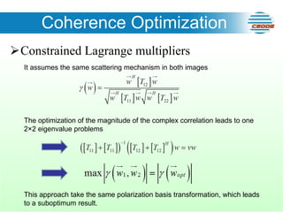
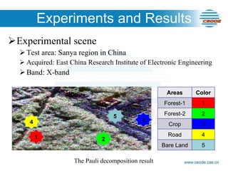
The document analyzes coherence optimization methods for compact polarimetric synthetic aperture radar interferometry (C-PolInSAR). It finds that while coherence is generally lower for C-PolInSAR than fully polarimetric SAR, optimization techniques can increase coherence to levels close to fully polarimetric SAR. The dual circular polarization mode provided the highest coherence for forested and crop areas, while the π/4 mode was best for roads and bare land. Coherence was highest using the unconstrained Lagrange multipliers method and decreased using the numerical radius and constrained Lagrange multipliers methods.

1. An Analysis of Coherence Optimization Methods in Compact Polarimetric SAR Interferometry Meng Liu,Hong Zhang,Chao Wang, Bo Zhang Vancouver, Canada July 29, 2011 IGRASS2011

2. Outline Introduction 1 2 3 Coherence Optimization of C-PolInSAR 4 Conclusions Experiments and Results

3. Introduction PolInSAR PolInSAR uses the interferometric degree of coherence estimated at different polarizations to extend the observation space of targets Promising applications, especially in the field of forest remote sensing Coherence optimization Technique to enhance the interferometric coherence It is achieved by the choice of a polarization basis within the polarimetric observation space.

4. Introduction Coherence optimization in fully PolInSAR system Unconstrained Lagrange multipliers method: the potential scattering mechanisms is different in both images Constrained Lagrange multipliers method: assuming the same scattering mechanism in both images Numerical radius method: gives a higher coherence than the constrained Lagrange multipliers method

5. Introduction Compact Polarimetry (CP) system A CP system transmits a wave on π/4 oriented linear or circular polarization, while receives the backward wave on two orthogonal linear or circular polarizations A CP system has advantage over a fully polarimetric (FP) system in terms of reductions of pulse repetition frequency, data volume, and system power needs

6. Introduction Three modes of CP C-PolInSAR π/4 mode: Dual Circular Polarimetric mode: right circular transmit, linear (horizontal and vertical) receive (CTLR) mode: C-PolInSAR InSAR CP

7. Introduction The workflow of C-PolInSAR Simulation Reconstruction reconstruction for coherence optimization Only two independent channels The assumption: reflection symmetry insignificance

8. Introduction Objective Solve the coherence optimization problem in C-PolInSAR without the reconstruction of the pseudo F-PolInSAR covariance matrix validation Compare coherence optimization of CP modes with the corresponding FP modes, as well as the conventional coherence optimization methods.

9. Coherence Optimization The complex correlation coefficient of CP The optimal coherent coefficient the highest correlation of the two images can be selected by tuning the w i polarization in each resolution element

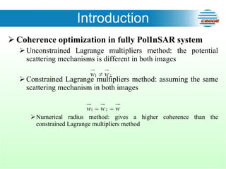
10. Coherence Optimization Unconstrained Lagrange multipliers Solving this equation leads to two 2×2 eigenvalue problems [A][B] is similar to [B][A], they have the same real nonnegative eigenvalues.

11. Coherence Optimization Constrained Lagrange multipliers It assumes the same scattering mechanism in both images The optimization of the magnitude of the complex correlation leads to one 2×2 eigenvalue problems This approach take the same polarization basis transformation, which leads to a suboptimum result.

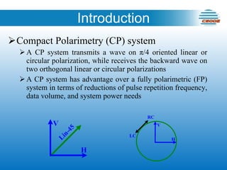
12. Coherence Optimization Numerical radius It provides a new thought to solve the constrained Lagrange multipliers function. Assumption: [T 11 ] is similar to [T 22 ] The maximum coherence corresponds to the numerical radius of the matrix [A] Define

13. Experiments and Results Experimental scene Test area: Sanya region in China Acquired: East China Research Institute of Electronic Engineering Band: X-band The Pauli decomposition result 1 2 3 4 5 Areas Color Forest-1 1 Forest-2 2 Crop 3 Road 4 Bare Land 5

14. Experiments and Results (a) FP case (c) DCP mode (b) π/4 mode (d) CTLR mode The histogram of FP case is right shifted compare to the position of any mode of CP cases The trend of the coherence histograms for CP case is closed to the corresponding FP case, no matter which method or CP mode was selected In most cases the ULM gives the highest coherence, followed by the NR and the CLM, this result is similar to the FP case.

15. Conventional Coherence VS FP Coherence Mean Coherence Values for Compact Polarimetric Modes the degree of coherence for any CP case is lower than the corresponding FP case, but it is higher than the conventional cases. The HH-VV conventional coherence seems to be the worst case in all case except for the road areas, where the HV conventional coherence is lowest. Among the three compact modes, the situation becomes complicated. The DCP mode gives the highest coherence over forest 1 and crop areas. For the low forest (forest 2) areas, the CTLR mode is slightly better than other modes. For the road and bare land areas, the π/4 mode seems to be the best compact mode. ROI Conventional Coherence FP Coherence HH HV VV HH+VV HH-VV ULM NR CLM forest 1 0.770 0.734 0.780 0.793 0.721 0.913 0.876 0.861 forest 2 0.809 0.774 0.796 0.817 0.750 0.924 0.892 0.870 crop 0.813 0.748 0.797 0.819 0.724 0.931 0.900 0.893 road 0.632 0.382 0.616 0.673 0.509 0.818 0.766 0.751 bare land 0.846 0.707 0.845 0.898 0.635 0.931 0.901 0.890 ROI Lin45 DCP CTLR ULM NR CLM ULM NR CLM ULM NR CLM forest 1 0.851 0.830 0.816 0.865 0.843 0.831 0.862 0.839 0.824 forest 2 0.874 0.855 0.836 0.880 0.863 0.845 0.881 0.861 0.846 crop 0.883 0.861 0.852 0.887 0.868 0.860 0.887 0.866 0.857 road 0.729 0.702 0.681 0.732 0.701 0.683 0.719 0.681 0.656 bare land 0.895 0.881 0.872 0.893 0.878 0.868 0.900 0.881 0.870

16. Conclusions 1 Compared with the FP case, one can observe that there is a significant loss in coherence of 5-10% when CP modes are available. 2 The trend of the coherence histograms for CP case is closed to the corresponding FP case, no matter which method or CP mode was selected. 3 It is shown that the degree of coherence from CP case carries enough information for some polarimetric SAR interferometry applications .