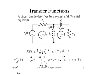
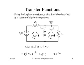
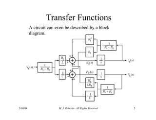
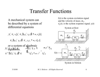
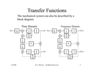
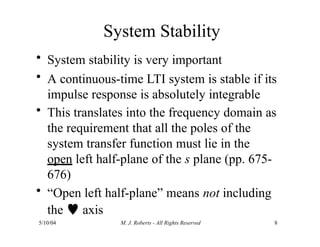
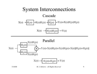
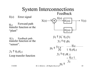
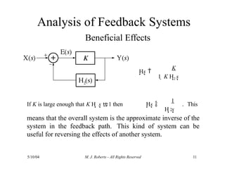
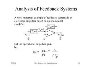
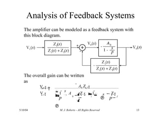
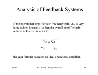
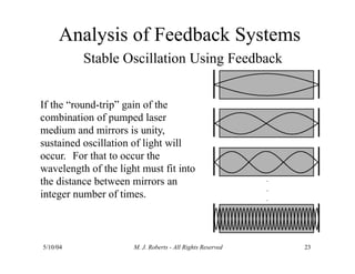
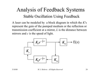
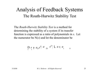
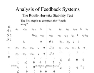
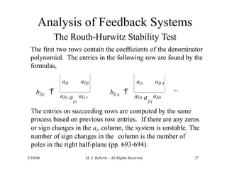
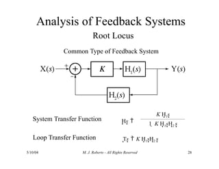
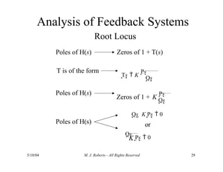
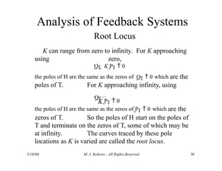
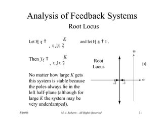
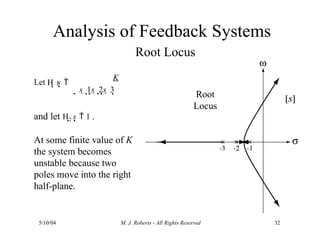
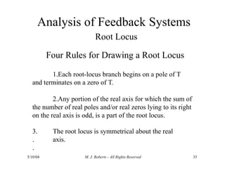
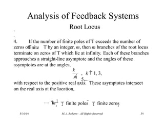
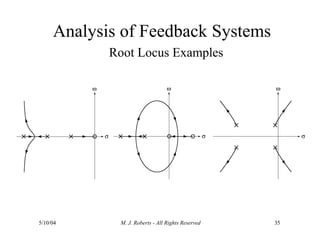
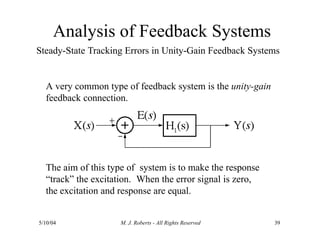
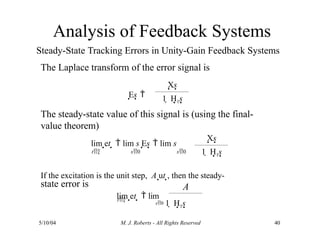
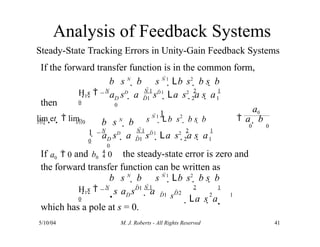
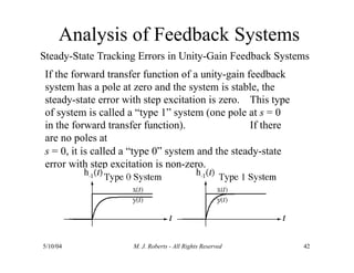
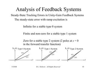
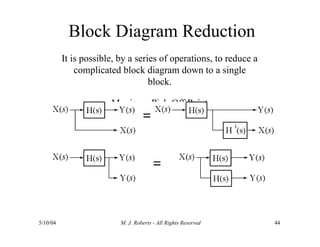
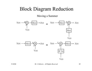
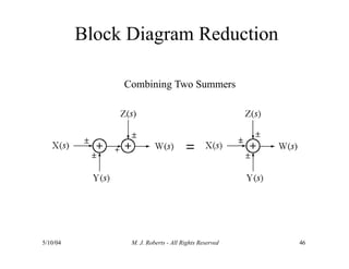
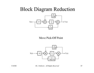
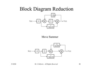
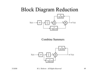
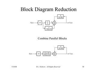
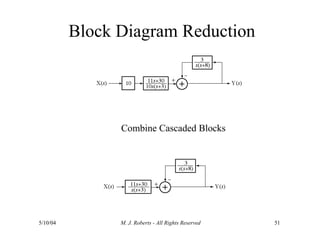
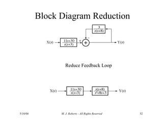
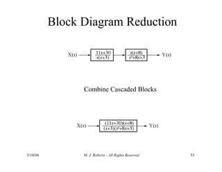
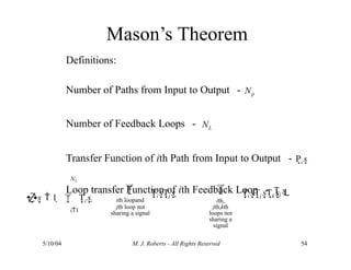
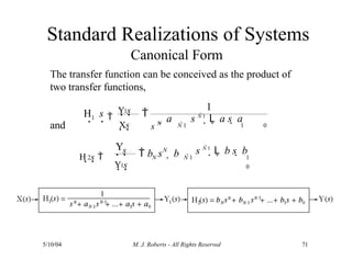
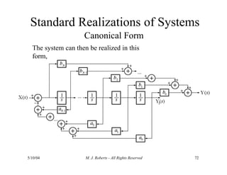
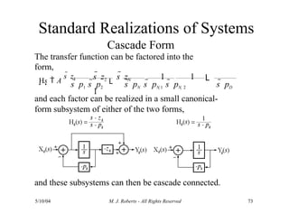
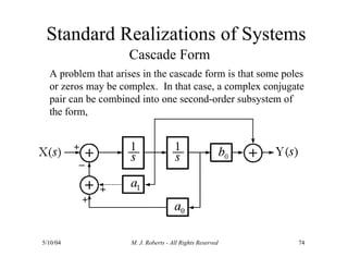
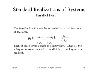
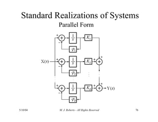
Sinyal sistem engineering Chapter10Slides.pptx

Laplace Transform Analysis of
Signals and Systems

Transfer Functions
5/10/04 M. J. Roberts - All Rights Reserved 2
• Transfer functions of CT systems can
be found from analysis of
– Differential Equations
– Block Diagrams
– Circuit Diagrams

Transfer Functions
A circuit can be described by a system of differential
equations
g
1 1
1
2 

R i t   L  d
i t  
d
i t   v t 
L

d

d
d
dt c
t
2
i t   1 2 2 2
1
i t 
dt
dt



   t   0

0
C

i d  v 0  R i

Transfer Functions
Using the Laplace transform, a circuit can be described
by a system of algebraic equations
R1 I1s  sL I1s  sL I2 s  Vg s
sC
2
1
2 2
2
sL I s  sL I s 
1
I s  R I s  0

A circuit can even be described by a block
diagram.
Transfer Functions

A mechanical system can
be described by a system of
differential equations
ft   Kd x1t   Ks1x1t   x2 t   m1 x1t
Ks1x1t   x2 t   Ks 2 x2 t   m2 x2 t
or a system of algebraic
equations.
m s X


Fs  K s X s  K X s  X s  s
K X s  X s  K X s  m s X s
d 1 s1
2
1 2 1 1
s1 1 2 s 2 2
2
2 2
Transfer Functions

The mechanical system can also be described by a
block diagram.
Time Domain Frequency Domain
Transfer Functions

System Stability
• System stability is very important
• A continuous-time LTI system is stable if its
impulse response is absolutely integrable
• This translates into the frequency domain as
the requirement that all the poles of the
system transfer function must lie in the
open left half-plane of the s plane (pp. 675-
676)
• “Open left half-plane” means not including
the  axis

System Interconnections
Cascade
Parallel

Feedback
Error signal
Es  Xs  H2 sYs
Ys  H sEs
1
Hs 
Ys 
H1s
Xs 1  H1sH2 s
E(s)
Forward path
transfer function or the
“plant”
2
transfer function or the
“sensor”.
H s Feedback path
Ts  H1sH2 s
Loop transfer function
H1s
H1s 1 
Ts
System Interconnections
Ts  H sH s
1
2
Hs 

Analysis of Feedback Systems
Beneficial Effects
Hs 
K
1  K H2 s
2
H s
If K is large enough that K H s  1 then Hs 
1
. This
2
means that the overall system is the approximate inverse of the
system in the feedback path. This kind of system can be
useful for reversing the effects of another system.

A very important example of feedback systems is an
electronic amplifier based on an operational
amplifier
Let the operational amplifier gain
be
1
H s 
A0
p
o
e
V s
V s
 
1 
s

The amplifier can be modeled as a feedback system with
this block diagram.
The overall gain can be written
as
Vi s
V0 s 
 A0 Z f s


  s


1 
s
 A Z s  1   Zs
p 0 
 i
 p f

If the operational amplifier low-frequency gain, A0 , is very
large (which it usually is) then the overall amplifier gain
reduces at low-frequencies to
V0 s  
Z f s
Vi s Zi s
the gain formula based on an ideal operational amplifier.

The change in overall system gain is about 0.001% for a
change in open-loop gain of a factor of 10.
The half-power bandwidth of the operational amplifier itself is
15.9 Hz (100/2).The half-power bandwidth of the overall
amplifier is approximately 14.5 MHz, an increase in
bandwidth of a factor of approximately 910,000.
0
0
If A 
106
If A  107
and p  100 then H j100  9.999989 
j0.000011 and p  100 then H j100  9.99989  j0.00011

Feedback can stabilize an unstable system. Let a forward-path
transfer function be
This system is unstable because it has a pole in the right
half- plane. If we then connect feedback with a transfer
function, K, a constant, the overall system gain becomes
s  p  K
and, if K > p, the overall system is now stable.
1
s  p
H s 
1
, p  0
Hs 
1

Feedback can make an unstable system stable but it can
also make a stable system unstable. Even though all the
poles
of the forward and feedback systems may be in the open
left half-plane, the poles of the overall feedback system can
be in the right half-plane.
A familiar example of this kind of instability caused by
feedback is a public address system. If the amplifier
gain is set too high the system will go unstable and
oscillate, usually with a very annoying high-pitched tone.

Public Address System
As the amplifier gain is
increased, any sound
entering the microphone
makes a stronger sound
from the speaker until, at
some gain level, the
returned sound from the
speaker is a large as the
originating sound into the
microphone. At that point
the system goes unstable
(pp. 685-689).

Stable Oscillation Using Feedback
Prototype
Feedback
System
Feedback
System
Without
Excitation

Can the response be non-zero when the
excitation is zero? Yes, if the overall
system gain is infinite. If the system
transfer function has a pole pair on the
axis, then the transfer function is
infinite
at the frequency of that pole pair and there can be a response
without an excitation. In practical terms the trick is to be sure
the
poles stay on the  axis. If the poles move into the left half-
plane
the response attenuates with time. If the poles move into the right
half-plane the response grows with time (until the system goes
non- linear).

A real example of a system that oscillates stably is a laser.
In a laser the forward path is an optical amplifier.
The feedback action is provided by putting mirrors at
each end of the optical amplifier.

Laser action begins when a photon is spontaneously emitted
from the pumped medium in a direction normal to the mirrors.

If the “round-trip” gain of the
combination of pumped laser
medium and mirrors is unity,
sustained oscillation of light will
occur. For that to occur the
wavelength of the light must fit into
the distance between mirrors an
integer number of times.

A laser can be modeled by a block diagram in which the K’s
represent the gain of the pumped medium or the reflection or
transmission coefficient at a mirror, L is the distance between
mirrors and c is the speed of light.

The Routh-Hurwitz Stability Test
The Routh-Hurwitz Stability Test is a method for
determining the stability of a system if its transfer
function is expressed as a ratio of polynomials in s. Let
the numerator be N(s) and let the denominator be
D s a s
D
D
D1
 a sD1
L a s  a
1 0
  

The first step is to construct the “Routh
array”.
D
D  1
D  2
D  3
⁝
2
1
0
aD aD2 aD 4 L a0
D aD1 aD 3 aD5
L 0 D  1
bD2 bD 4 bD6 L 0 D  2
cD 3 cD5 cD 7 L 0 D  3
⁝ ⁝ ⁝ ⁝ ⁝ ⁝
d2 d0 0 0 0 2
e1 0 0 0 0 1
f0 0 0 0 0 0
aD aD2 aD 4 L a1
aD1 aD 3 aD5 L a0 bD2
bD 4 bD6 L 0
cD 3 cD5 cD 7 L 0
⁝ ⁝ ⁝ ⁝
⁝
d2 d0 0 0
0
e1 0 0 0
0

The first two rows contain the coefficients of the denominator
polynomial. The entries in the following row are found by the
formulas,
b  
a
aD aD2
aD1 aD 3
D2
a
b  
D 4
aD aD 4
aD1 aD5
D1 D1
...
The entries on succeeding rows are computed by the same
process based on previous row entries. If there are any zeros
or sign changes in the aD column, the system is unstable. The
number of sign changes in the column is the number of
poles in the right half-plane (pp. 693-694).

Root Locus
Common Type of Feedback System
System Transfer Function Hs 
K H1s
1  K H1sH2 s
Loop Transfer Function Ts  K H1sH2 s

Root Locus
Poles of H(s) Zeros of 1 + T(s)
T is of the form
Ts  K
Ps
Qs
Poles of H(s)
Zeros of 1 + K
Ps
Qs
Poles of H(s)
Qs  K Ps  0
or
K
Qs  Ps  0

Root Locus
K can range from zero to infinity. For K approaching
zero,
using
the poles of H are the same as the zeros of Qs  0 which are the
poles of T. For K approaching infinity, using
Qs  K Ps  0
K
Qs  Ps  0
the poles of H are the same as the zeros of Ps  0 which are the
zeros of T. So the poles of H start on the poles of
T and terminate on the zeros of T, some of which may be
at infinity. The curves traced by these pole
locations as K is varied are called the root locus.

Root Locus
Then Ts 
K
No matter how large K gets
this system is stable because
the poles always lie in the
left half-plane (although for
large K the system may be
very underdamped).
1
s  1s  2
2
Let H s 
K
and let H s  1 .
s  1s  2 Root
Locus

Root Locus
Root
Locus
and let H2 s  1 .
At some finite value of K
the system becomes
unstable because two
poles move into the right
half-plane.
1
Let H s 
K
s  1s  2s  3

Root Locus
Four Rules for Drawing a Root Locus
1.Each root-locus branch begins on a pole of T
and terminates on a zero of T.
2.Any portion of the real axis for which the sum of
the number of real poles and/or real zeros lying to its right
on the real axis is odd, is a part of the root locus.
3.
.
.
The root locus is symmetrical about the real
axis.

.
.
4. If the number of finite poles of T exceeds the number of
finite
zeros of T by an integer, m, then m branches of the root locus
terminate on zeros of T which lie at infinity. Each of these branches
approaches a straight-line asymptote and the angles of these
asymptotes are at the angles,
k

m
, k  1, 3,
5,...
Root Locus
m
with respect to the positive real axis. These asymptotes intersect
on the real axis at the location,
 
1
finite poles  finite zeros

Root Locus Examples

Gain and Phase Margin
Real systems are usually designed with a margin of error
to allow for small parameter variations and still be stable.
That “margin” can be viewed as a gain margin or a phase
margin.
System instability occurs if, for any real ,
T j   1
a number with a magnitude of one and a phase of -
 radians.

So to be guaranteed stable, a system must have a T whose
magnitude, as a function of frequency, is less than one when
the phase hits - or, seen another way, T must have a phase,
as
a function of frequency, more positive than -  for all |
T| greater than one.
The difference between the a magnitude of T of 0 dB and
the magnitude of T when the phase hits -  is the gain
margin.
The difference between the phase of T when the
magnitude hits 0 dB and a phase of -  is the phase
margin.

Steady-State Tracking Errors in Unity-Gain Feedback Systems
A very common type of feedback system is the unity-gain
feedback connection.
The aim of this type of system is to make the response
“track” the excitation. When the error signal is zero,
the excitation and response are equal.

The Laplace transform of the error signal is
The steady-state value of this signal is (using the final-
value theorem)
state error is
If the excitation is the unit step, A ut , then the steady-
Es 
Xs
1  H1s
lim et   lim s Es  lim s
t s0 s0
Xs
1  H1s
A
t
lim et   lim
s0 1  H1s

If the forward transfer function is in the common form,
then
which has a pole at s = 0.
a sD
 a
H1s  N N 1 2 1
0
D D1 2 1
0
b s N
 b s N 1
Lb s2
 b s  b
sD1
La s2
 a s  a
b s N
 b
a sD
 a
t s0
D D1 2 1
0
lim et   lim
1

1  N N 1 2 1
0
s N 1
Lb s2
 b s  b a  b
0 0
sD1
La s2
 a s  a
If a0  0 and b0  0 the steady-state error is zero and
the forward transfer function can be written as
a0
2 1
s a s
D  a

H1s  N N 1 2 1
0
D1
D1 sD2
b s N
 b s N 1
Lb s2
 b s  b
La s  a 

If the forward transfer function of a unity-gain feedback
system has a pole at zero and the system is stable, the
steady-state error with step excitation is zero. This type
of system is called a “type 1” system (one pole at s = 0
in the forward transfer function). If there
are no poles at
s = 0, it is called a “type 0” system and the steady-state
error with step excitation is non-zero.

The steady-state error with ramp excitation is
Infinite for a stable type 0 system
Finite and non-zero for a stable type 1 system
Zero for a stable type 2 system (2 poles at s = 0
in the forward transfer function)

Block Diagram Reduction
It is possible, by a series of operations, to reduce a
complicated block diagram down to a single
block.
Moving a Pick-Off Point

Moving a Summer

Combining Two Summers

Move Pick-Off Point

Move Summer

Combine Summers

Combine Parallel Blocks

Combine Cascaded Blocks

Reduce Feedback Loop

Combine Cascaded Blocks

Mason’s Theorem
Definitions:
Number of Paths from Input to Output - Np
Number of Feedback Loops - NL
Transfer Function of ith Path from Input to Output - Pi s
Loop transfer Function of ith Feedback Loop - Ti s
Ti sTj s 
NL
s  1   Ti s 
i1

ith loopand
jth loop not
sharing a signal

ith,
jth,kth
loops not
sharing a
signal
Ti sTj sTk s  L

Mason’s Theorem
The overall system transfer function
is
Hs 
N p
Pi si s
s
i1
where i s is the same as s except that all feedback loops
which share a signal with the ith path, Pi s, are
excluded.

Mason’s Theorem
1
s
P s 
10
2
P s 
1
s  3
Np  2 NL 
1
s s  8
s  1 
1 3
 1 
3
ss  8
1s  2 s  1
N p
Pi si s
s
10

1
Hs  i1  s s  3 
3
ss  8
s  811s  30
s  3s2
 8s  3
1 

System Responses to Standard Signals
Unit Step Response
Let Hs 
Ns be proper in s. Then the Laplace
transform
Ds
of the unit step response is
Ys  H
s Ds Ds s
1 s 
Ns 
N1s 
K
If the system is stable, the inverse Laplace transform of
N1s
Ds
is called the transient response and the steady-state
response is H0 .
s
K  H0

Let Hs 
Ns be proper in s. If the Laplace transform of
the
Ds
excitation is some general excitation, X(s), then the
Laplace transform of the response is
Ds Ds Dx s Ds Dx s
Ys 
Ns Xs 
Ns N x s 
N1s 
N x1s
123
same poles
as system
123
same poles
as excitation

p
1 
s
Unit Step Response
Let Hs 
A
. Then the unit step response is yt   A1  ept
ut 

Unit Step Response
Let
s  0
A
2
s2 0 0
 2 s  
2
(pp. 710-712)

Let s  0
s2 0 0
 2 s  
2
Unit Step Response
A 2

Let Hs 
Ns be proper in s. If the excitation is a
suddenly-
Ds
applied, unit-amplitude cosine, the response is
If the system is stable, the steady-state response is a sinusoid of
same frequency as the excitation but, generally, a different
magnitude and phase.
s
Ys 
Ns
0
which can be reduced and inverse Laplace transformed
into (pp. 713-714)
Ds s2
  2
y
 H j
t  
 
 N s


 Ds


     t 
C1
1
0 0
0
 cos

t  H j u

Pole-Zero Diagrams and
Frequency Response
If the transfer function of a system is H(s), the frequency
response is H(j). The most common type of transfer
function
is of the form,
Hs  A
s  z1 s  z2 Ls  zN 
s  p1 s  p2 Ls  pD 
Therefore H(j) is
H j   A
 j  z1  j  z2 L j  zN 
 j  p1  j  p2 L j  pD 

Frequency Response
Let Hs 
3s
s  3
j
j  3
H j   3
The numerator, j, and
the denominator, j  ,
can be conceived as
vectors in the
s plane.
H j   3
j

j  3 H j   {3  j   j  3
0

Frequency Response

0
lim H j   lim 3
 0
 0
j

j  3

0
lim H j   lim 3
 0
 0
j

j  3
lim H j

  lim 3 j 
3


  j  3
j

lim H j   lim
3
   
j  3
 3

Frequency Response
 0
2 2
lim H j  

 0 

 0
2 2
lim H j   

 0  



2  2

lim H j   

  
   0 

2 2
lim H j  



 0

Butterworth Filters
The squared magnitude of the transfer function of an nth order,
unity-gain, lowpass Butterworth filter with a corner frequency
of 1 radian/s is
This is called a normalized
Butterworth filter because
its gain is normalized to
one and its corner
frequency
is normalized to
1 radian/s.
H j 2

1
1   2n

Butterworth Filters
A Butterworth filter transfer function has no finite zeros
and the poles all lie on a semicircle in the left-half plane
whose radius is the corner frequency in radians/s and the
angle between the pole locations is always /n radians.

Butterworth Filters
Frequency Transformations
A normalized lowpass Butterworth filter can be transformed
into an unnormalized highpass, bandpass or bandstop Butterworth
filter through the following transformations (pp. 721-725).
Lowpass to Highpass
Lowpass to Bandpass
Lowpass to Bandstop
s
s 
c
s  L H
s2  

s H   L 
L H
s 
s H   L 
 

s2

Standard Realizations of Systems
There are multiple ways of drawing a system block
diagram corresponding to a given transfer function of the
form,
Hs 
Ys
Xs
, aN 
1
b s
k
k
N
k
N
s N
b s N
 b

ak
s
k 0
 k 0  N N 1 1 0
N 1 1 0
s N 1
L b s  b
 a s N 1
L a s  a

Canonical Form
The transfer function can be conceived as the product of
two transfer functions,
and
1
H s 1
Y s
Xs
1
s N N 1
 a s N 1
L a s  a
1 0
   
Y
2
H s 
1
s
Y s
N
N
 b s  b N 1
s N 1
L b s  b
1
0

Canonical Form
The system can then be realized in this
form,

Cascade Form
The transfer function can be factored into the
form,
and each factor can be realized in a small canonical-
form subsystem of either of the two forms,
and these subsystems can then be cascade connected.
Hs  A
s  z1
s  p1 s  p2 s  pN s  pN 1 s  pN  2 s  pD
s  z2
L
s  zN 1 1
1
L

Cascade Form
A problem that arises in the cascade form is that some poles
or zeros may be complex. In that case, a complex conjugate
pair can be combined into one second-order subsystem of
the form,

Parallel Form
The transfer function can be expanded in partial fractions
of the form,
Each of these terms describes a subsystem. When all the
subsystems are connected in parallel the overall system is
realized.
Hs 
KD
s  pD
K1

K2
s  p1 s  p2
L

Parallel Form

State-Space Analysis
• In larger systems it is important to keep the
analysis methods systematic to avoid
errors
• One popular method for doing this is
through the use of state variables
• State variables are signals in a system
which, together with the excitations,
completely characterize the state of the
system
• As the system changes dynamically the state
variables change value and the system
moves on a trajectory through state space

• State space is an N-dimensional space
where
N is the order of the system
• The order of a system is the number of
state variables needed to characterize it
• State variables are not unique, there can
be multiple correct sets

• There are several advantages to state-
space analysis
– Reduction of the probability of analysis errors
– Complete description of the system signals
– Insight into system dynamics
– Can be formulated using matrix methods and the
system state can be expressed in two
matrix equations
– Combined with transform methods it is very
powerful

To illustrate state-space methods, let the system be this circuit
Let the state variables be the capacitor voltage and the
inductor current and let the output signals be vout t  and iR t .

Two differential equations in the two state variables, called the
state equations, characterize the circuit,
Two more equations called the output equations define the
responses in terms of the state variables,
vout t   vC t  iR t   G vC t 
L C
L
it  
1
v t  C L C in
C C C
vt   
1
i t  
G
v t  
1
i t 

The state equations can be written in matrix form
as





L
C
L
C
in
 it 

vt

L



C

C 
 
and the output equations can be written in matrix
form as
G v
t 

C


0
1 
 i
t  
1
 0

  1 i
t 
i
R
L
C
in


 i t   

G 

v
t 

  

t 


vout t 

0  


0
1 i t 0

0



A block diagram for the
system can be drawn
directly from the state
and output equations.

L
C
qt   



 i
t 

v t 
A 

0
The state and output equations can be written compactly as
qt   Aqt   Bxt  yt  
Cqt   Dxt 
where
1



1
L


G 
 0 
B   1

C

xt   iin t 
yt  
R





vout t

i t 
C 

0
C C 
0
1 
G 
0

D 

0


or
The solution of the state and output equations can be
found using the Laplace transform.
sQs  q0
  AQs  BXs
sI  AQs  BXs  q0

Multiplying both sides bysI  A1
Qs  sI  A1
BXs  q0

The matrix, sI  A1
, is conventionally designated by the
symbol, s . Then
Q BX


  



s  s BX 

s s  s
s  q 0 q 0
1–2–3
zerostate
response
1–2 –3
zeroinput
response

The time-domain solution is then
where t 
C
 s and t is called the state transition matrix.
1–2–3
zerostate
response
1–2 –3
zeroinput
response
qt   t  Bxt   t q0


To make the example concrete, let the excitation and initial
conditions be
it   A ut 
0


1



 

 
q0
  





 i 0
v 0
L
C
3
and let R 
1
, C  1 , L  1
s  sI  A

C
s 
C

L

G

C
C
s 
G

 s 

 
1
1

1





L

 s 
s2
1



1
s



G
1
1

Solving for the states in the Laplace domain,

 C LC



s 

G
C LC

s 



Qs  




C LC
 






sLC s 
G
s 
1
 1 s
1 


G 1
C
LC
1 1
2
L s2

G
s 
1 

C s2
 s2
Substituting in numerical component values,


 
s

 3s  1
1 1
 3s  1

1
Qs 
 ss2 s2


 s2
 3s  1  3s  1

s2

Inverse Laplace transforming, the state variables
are
and the response is
yt  

0
or
 0.277e2.62 t

qt   

ut 
1  0.277e2.62 t
 0.723e0.382 t

0.723e0.382 t
 0.277e2.62 t
0

0 1 
0 G 

q 

0

x 

0
 
3


ut 
11  0.277e2.62 t
 0.723e0.382 t

0.723e0.382 t
yt  
0.723e0.382 t
 0.831e 2.62 t


2.169e0.382 t


ut 
 0.277e2.62 t


In a system in which the initial conditions are zero (the
zero-input response is zero), the matrix transfer
function can be found from the state and output
equations.
or
The response is
Ys  CQs  DXs  CsBXs  DXs  CsB  DXs
and the matrix transfer function is
Hs  CsB  D
sQs  q0
  AQs  BXs
123
0
Qs  sI  A1
BXs 
sBXs

Any set of state variables can be transformed into another
valid set through a linear transformation. Let q1t  be the initial
set and let q2 t  be the new set, related to q1t  by
q2 t   Tq1t 
Then
q2 t   Tq1t   TA1q1t   B1xt   TA1q1t   TB1xt 
and using q
2
where
1
2
t  T q t ,
   
1
1
1 2 1 2 2
2
qt   TA T q t   TB xt   A q t   B xt 
A  TA T1
2 1 B2  TB1

By a similar argument,
yt   C2q2 t   D2xt 
where
Transformation to a new set of state variables does not
change the eigenvalues of the system.
C  C T1
2 1 D2  D1

Sinyal sistem engineering Chapter10Slides.pptx

More Related Content

Similar to Sinyal sistem engineering Chapter10Slides.pptx

More from Mariya Nasution

Recently uploaded

Sinyal sistem engineering Chapter10Slides.pptx