Teaching the Correlation Coefficient
•
1 like•1,677 views

Teaching the meaning of the correlation coefficient is difficult enough without having to use a confusing formula for it. This "introduces" a "new" equation whose very form helps explain the meaning of the correlation coefficient.

More Related Content
What's hot
Viewers also liked
Similar to Teaching the Correlation Coefficient
Similar to Teaching the Correlation Coefficient (20)
More from John Zorich, MS, CQE
Teaching the Correlation Coefficient
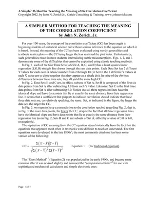
- 1. A Simpler Method for Teaching the Meaning of the Correlation Coefficient Copyright 2012, by John N. Zorich Jr., Zorich Consulting & Training, www.johnzorich.com ----------------------------------------------------------------------------------------------------------------------------------- A SIMPLER METHOD FOR TEACHING THE MEANING OF THE CORRELATION COEFFICIENT by John N. Zorich, Jr. For over 100 years, the concept of the correlation coefficient (CC) has been taught to beginning students of statistical science but without serious reference to the equation on which it is based. Instead, the meaning of the CC has been explained using wordy generalities and textbook scatter plots ⎯ the CC being larger the less scattered the plot looks. Unfortunately, such generalities result in most students internalizing subtle misconceptions. Figs. 1, 2, and 3 demonstrate some of the difficulties that cannot be explained using classic teaching methods. In Fig. 1, each of the four Data Sets (labeled A, B, C, and D) has a least squares linear regression (LSLR) straight line drawn through the raw data points. Each Data Set has 2 different Y values for each even X whole number from 2 through 18 (in Set D, the 2 different Y values at each X value are so close together that they appear as a single dot). In spite of the obvious differences between these data sets, they all yield the same high CC. In Fig. 2, Data Sets B and C are, in effect, subsets of Set A. Set B is composed of the first six data points from Set A after subtracting 3.0 from each Y value. Likewise, Set C is the first three data points from Set A after subtracting 6.0. Notice that all three regression lines have the identical slope and have data points that lie at exactly the same distance from their regression line. It seems that a coefficient that purports to indicate correlation should indicate that these three data sets are, correlatively speaking, the same. But, as indicated in the figure, the larger the data set, the larger the CC. In Fig. 3, we seem to have a contradiction to the conclusion reached regarding Fig. 2; that is, in Fig. 3, the more data points, the lower the CC, despite the fact that all three regression lines have the identical slope and have data points that lie at exactly the same distance from their regression line (as in Fig. 2, Sets B and C are subsets of Set A, offset by a value of 3.0 or 6.0, respectively). The separation of CC meaning from the CC equation stems historically from the fact that the equations that appeared most often in textbooks were difficult to teach or understand. The first equations were developed in the late 1800s1; the most commonly cited one has been some version of the following: ∑ ( X − X )( Y − Y ) CC = Equation 1 (the traditional equation) ∑ ( X − X ) ∑ (Y − Y ) 2 2 The “Short Method” 2 (Equation 2) was popularized in the early 1900s, and became more common after it was revised slightly and renamed the “computational form”3 for use with sophisticated mechanical calculators and simple electronic ones: Page 1 of 7
- 2. A Simpler Method for Teaching the Meaning of the Correlation Coefficient Copyright 2012, by John N. Zorich Jr., Zorich Consulting & Training, www.johnzorich.com ----------------------------------------------------------------------------------------------------------------------------------- N ∑ XY − ∑ X ∑ Y CC = Equation 2 ⎛ ⎞⎛ ⎞ ⎜ N ∑ X − (∑ X )2⎟⎜ N ∑ Y − (∑ Y )2⎟ 2 2 ⎝ ⎠⎝ ⎠ A simpler equation4 (Equation 3) was developed, but it didn’t have much pedagogic value. In this equation, Sx and Sy are the standard deviation of the X and Y data, respectively, and “slope” is the slope of the linear regression line calculated by the method of least squares: (slope)Sx CC = Equation 3 Sy The ratio of slope to Sy in this equation is helpful in explaining the lack of dependence of the CC on slope, since a large CC can result from either a large slope, a large Sx, and/or a small Sy. This equation is unable to explain what the CC is, but is wonderful for explaining what the CC is not. About 1985, I thought I’d developed a new, more instructive equation. Alas, a few years later, I found my “new” equation at the end of an appendix to a 1961 introductory statistics book written by someone else.5 I discovered my “new” equation within the equation for the Coefficient of Determination (CD). In the CD equation (see next), Ye represents the Y values calculated for each X value by using the least squares linear regression analysis equation (Ye = a + bX), and Yi represents the raw Y data. One Ye value is calculated for each Yi value. As always in least squares linear regression, the mean of the Ye data is the same as that of the Yi, and so it is not subscripted in the equation below: = CC 2 = ( ∑ Ye − Y )2 Equation 4 CD ∑ (Yi − Y ) 2 Dividing top and bottom of the fraction by N-1 (where N is the number of Yi data points), I discovered an equation that is the ratio of two sample variances: V a ria n c e ( Y e ) CC 2 = Equation 5 V a ria n c e ( Y i ) After taking the square root of both sides, I found an equation containing the absolute value of the CC on one side, and the ratio of two sample standard deviations on the other: S td D e v ia tio n ( Y e ) CC = Equation 6 (the “new” equation) S td D e v ia tio n ( Y i ) Page 2 of 7
- 3. A Simpler Method for Teaching the Meaning of the Correlation Coefficient Copyright 2012, by John N. Zorich Jr., Zorich Consulting & Training, www.johnzorich.com ----------------------------------------------------------------------------------------------------------------------------------- Although this equation does not calculate the sign of the CC, this is not a limitation. In LSLR, the sign of the CC is always the same as that of the regression coefficient (“b” in the LSLR equation Y= a + bX) — that is, if the slope is negative, so is the CC, and vice versa, as easily seen from Equation 3, above. Thus, the sign of the CC has no meaning independent of the regression slope, and so the only unique aspect of the CC is its absolute value, which the “new” equation calculates. Calculation of the CC using the new equation is shown by example in Table 1. Not only can this new equation be used to easily explain the surprising CC results shown in Figs. 1, 2, and 3, but it can also be use to explain other interesting facts, such as: 1. The correlation coefficient can never equal exactly 1.000, unless all the Yi’s form a perfectly straight line ⎯ which is the only case in which the standard deviations of Ye and Yi are identical. 2. The CC can never equal exactly 0.000, unless the standard deviation of Ye is also zero ⎯ which would occur only if the calculated linear regression line were perfectly horizontal. 3. The CC represents the fraction of the total variation in Yi, as measured in units of standard deviation, that can be explained by a linear relationship between Yi and X. The larger the CC, the larger the fraction of the Yi variation which can be explained this way. The remaining variation can’t be explained, at least not by the CC. Page 3 of 7
- 4. A Simpler Method for Teaching the Meaning of the Correlation Coefficient Copyright 2012, by John N. Zorich Jr., Zorich Consulting & Training, www.johnzorich.com ----------------------------------------------------------------------------------------------------------------------------------- Fig. 1 Linear Regression by Least Squares Correlation Coefficient = 0.955 for Each Data Set 14 A 12 10 B 8 6 C 4 2 D 0 0 2 4 6 8 10 12 14 16 18 20 Page 4 of 7
- 5. A Simpler Method for Teaching the Meaning of the Correlation Coefficient Copyright 2012, by John N. Zorich Jr., Zorich Consulting & Training, www.johnzorich.com ----------------------------------------------------------------------------------------------------------------------------------- Fig. 2 14 Linear Regression by Least Squares 12 A 10 8 B 6 4 Correlation Coefficients Data Set A = 0.955 Data Set B = 0.906 C Data Set C = 0.714 2 0 0 2 4 6 8 10 12 14 16 18 20 Page 5 of 7
- 6. A Simpler Method for Teaching the Meaning of the Correlation Coefficient Copyright 2012, by John N. Zorich Jr., Zorich Consulting & Training, www.johnzorich.com ----------------------------------------------------------------------------------------------------------------------------------- Fig. 3 Linear Regression by Least Squares 14 Correlation Coefficients Data Set A = 0.955 Data Set B = 0.962 12 Data Set C = 0.971 A 10 B 8 6 C 4 2 0 0 2 4 6 8 10 12 14 16 18 20 Page 6 of 7
- 7. A Simpler Method for Teaching the Meaning of the Correlation Coefficient Copyright 2012, by John N. Zorich Jr., Zorich Consulting & Training, www.johnzorich.com ----------------------------------------------------------------------------------------------------------------------------------- Table 1. Calculation of the Correlation Coefficient using the “New Equation” (Ye is calculated using the regression equation at the bottom of this table) X raw data Yi raw data Ye, calculated 6 10 9.7609 7 11 10.2065 7 10 11.5435 8 11 11.5435 9 12 11.5435 10 12 11.9891 10 12 12.4348 12 13 12.8804 13 14 13.3261 15 14 13.7717 Standard Deviation = Standard Deviation = 1.4491 1.4023 Least Squares Linear Regression Equation is Ye = 7.2221 + 0.4823X Correlation Coefficient (CC) using the “Traditional Equation” = 0.9677 CC using the “New Equation,” (StdDev Ye) / (StdDev Yi) = 0.9677 1 S. M. Stigler, The History of Statistics, 1986 (Belknap Press, Cambridge MA), chapter 9. 2 J. G. Smith, Elementary Statistics, 1934 (Henry Holt & Co., New York) p. 374. 3 H. L. Alder, E. B. Roessler, Introduction to Probability and Statistics, 6th ed., 1977 (W. H. Freeman & Co., San Francisco) p. 230. 4 Ibid, p. 231. Alder & Roessler use different symbols than are used here. 5 W. J. Reichmann, Use and Abuse of Statistics, 1961 (Oxford University Press, New York) p. 306. Page 7 of 7