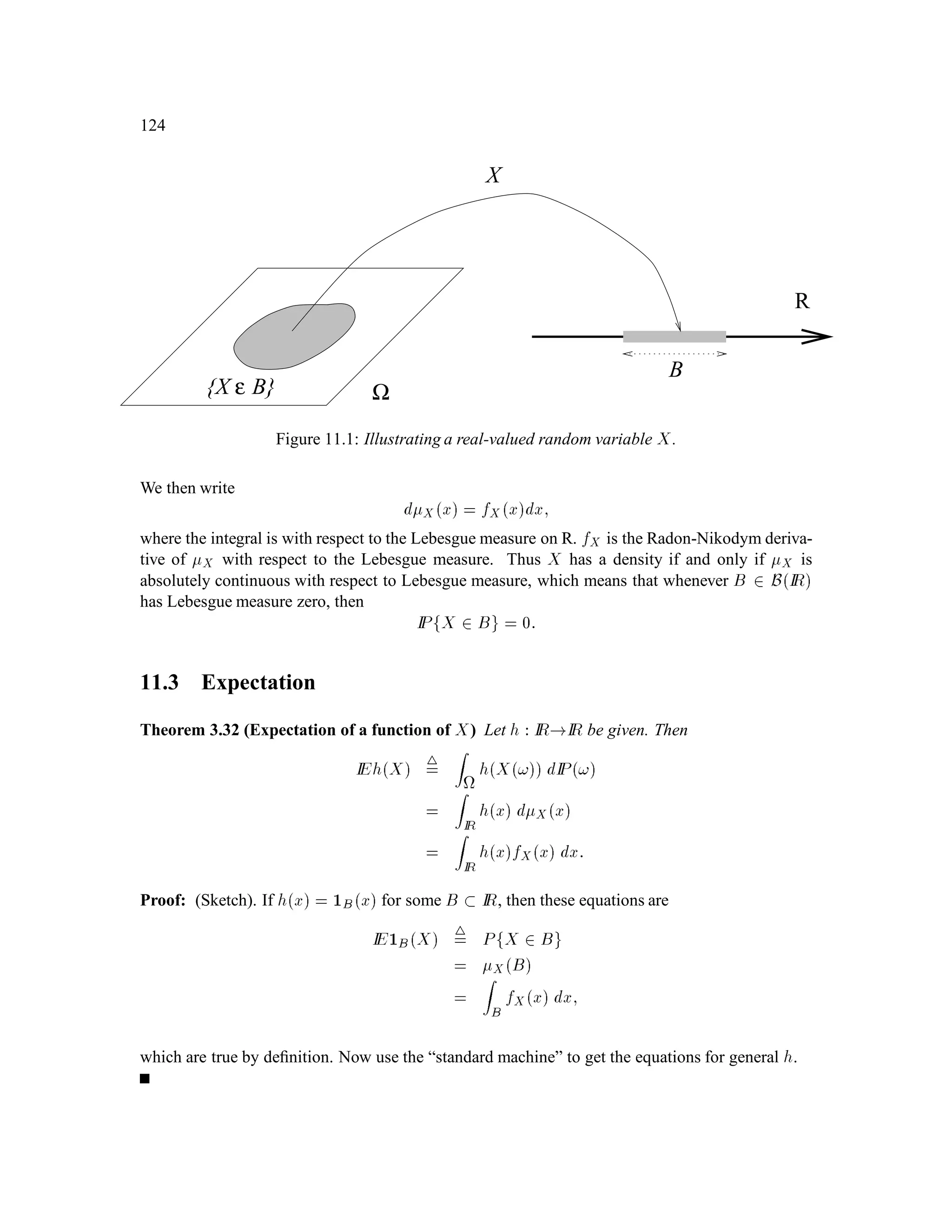
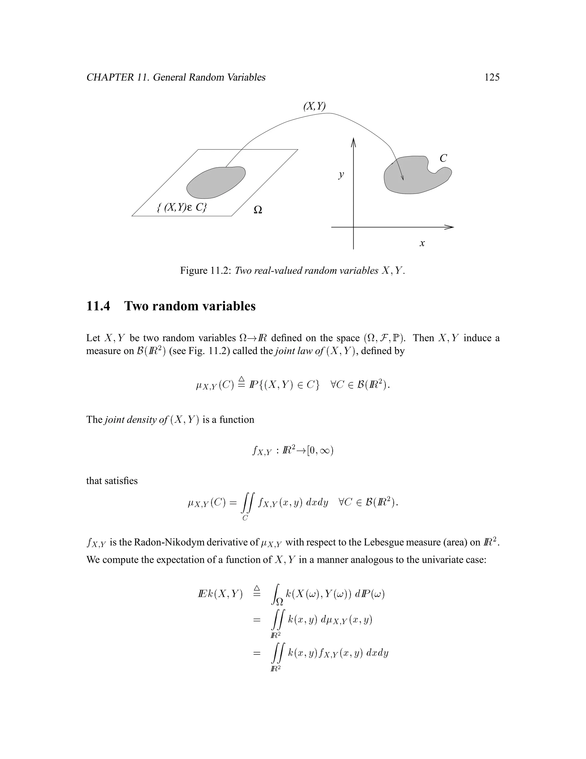
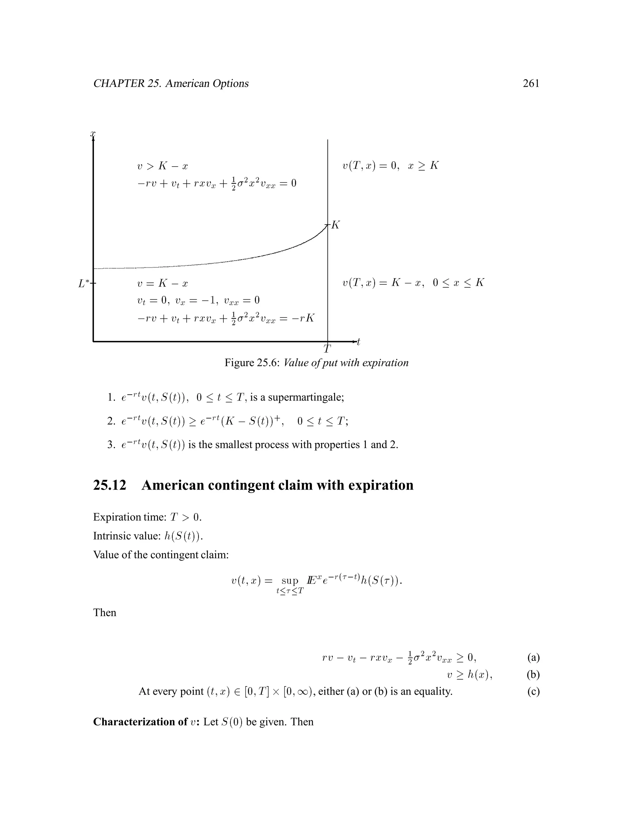
Steven Shreve: Stochastic Calculus and Finance
PRASAD CHALASANI
Carnegie Mellon University
chal@cs.cmu.edu
SOMESH JHA
Carnegie Mellon University
sjha@cs.cmu.edu
c Copyright; Steven E. Shreve, 1996
July 25, 1997
Contents
1 Introduction to Probability Theory 11
1.1 The Binomial Asset Pricing Model . . . . . . . . . . . . . . . . . . . . . . . . . . 11
1.2 Finite Probability Spaces . . . . . . . . . . . . . . . . . . . . . . . . . . . . . . . 16
1.3 Lebesgue Measure and the Lebesgue Integral . . . . . . . . . . . . . . . . . . . . 22
1.4 General Probability Spaces . . . . . . . . . . . . . . . . . . . . . . . . . . . . . . 30
1.5 Independence . . . . . . . . . . . . . . . . . . . . . . . . . . . . . . . . . . . . . 40
1.5.1 Independence of sets . . . . . . . . . . . . . . . . . . . . . . . . . . . . . 40
1.5.2 Independence of -algebras . . . . . . . . . . . . . . . . . . . . . . . . . 41
1.5.3 Independence of random variables . . . . . . . . . . . . . . . . . . . . . . 42
1.5.4 Correlation and independence . . . . . . . . . . . . . . . . . . . . . . . . 44
1.5.5 Independence and conditional expectation. . . . . . . . . . . . . . . . . . 45
1.5.6 Law of Large Numbers . . . . . . . . . . . . . . . . . . . . . . . . . . . . 46
1.5.7 Central Limit Theorem . . . . . . . . . . . . . . . . . . . . . . . . . . . . 47
2 Conditional Expectation 49
2.1 A Binomial Model for Stock Price Dynamics . . . . . . . . . . . . . . . . . . . . 49
2.2 Information . . . . . . . . . . . . . . . . . . . . . . . . . . . . . . . . . . . . . . 50
2.3 Conditional Expectation . . . . . . . . . . . . . . . . . . . . . . . . . . . . . . . 52
2.3.1 An example . . . . . . . . . . . . . . . . . . . . . . . . . . . . . . . . . . 52
2.3.2 Definition of Conditional Expectation . . . . . . . . . . . . . . . . . . . . 53
2.3.3 Further discussion of Partial Averaging . . . . . . . . . . . . . . . . . . . 54
2.3.4 Properties of Conditional Expectation . . . . . . . . . . . . . . . . . . . . 55
2.3.5 Examples from the Binomial Model . . . . . . . . . . . . . . . . . . . . . 57
2.4 Martingales . . . . . . . . . . . . . . . . . . . . . . . . . . . . . . . . . . . . . . 58
1
2
3 Arbitrage Pricing 59
3.1 Binomial Pricing . . . . . . . . . . . . . . . . . . . . . . . . . . . . . . . . . . . 59
3.2 General one-step APT . . . . . . . . . . . . . . . . . . . . . . . . . . . . . . . . . 60
3.3 Risk-Neutral Probability Measure . . . . . . . . . . . . . . . . . . . . . . . . . . 61
3.3.1 Portfolio Process . . . . . . . . . . . . . . . . . . . . . . . . . . . . . . . 62
3.3.2 Self-financing Value of a Portfolio Process  . . . . . . . . . . . . . . . . 62
3.4 Simple European Derivative Securities . . . . . . . . . . . . . . . . . . . . . . . . 63
3.5 The Binomial Model is Complete . . . . . . . . . . . . . . . . . . . . . . . . . . . 64
4 The Markov Property 67
4.1 Binomial Model Pricing and Hedging . . . . . . . . . . . . . . . . . . . . . . . . 67
4.2 Computational Issues . . . . . . . . . . . . . . . . . . . . . . . . . . . . . . . . . 69
4.3 Markov Processes . . . . . . . . . . . . . . . . . . . . . . . . . . . . . . . . . . . 70
4.3.1 Different ways to write the Markov property . . . . . . . . . . . . . . . . 70
4.4 Showing that a process is Markov . . . . . . . . . . . . . . . . . . . . . . . . . . 73
4.5 Application to Exotic Options . . . . . . . . . . . . . . . . . . . . . . . . . . . . 74
5 Stopping Times and American Options 77
5.1 American Pricing . . . . . . . . . . . . . . . . . . . . . . . . . . . . . . . . . . . 77
5.2 Value of Portfolio Hedging an American Option . . . . . . . . . . . . . . . . . . . 79
5.3 Information up to a Stopping Time . . . . . . . . . . . . . . . . . . . . . . . . . . 81
6 Properties of American Derivative Securities 85
6.1 The properties . . . . . . . . . . . . . . . . . . . . . . . . . . . . . . . . . . . . . 85
6.2 Proofs of the Properties . . . . . . . . . . . . . . . . . . . . . . . . . . . . . . . . 86
6.3 Compound European Derivative Securities . . . . . . . . . . . . . . . . . . . . . . 88
6.4 Optimal Exercise of American Derivative Security . . . . . . . . . . . . . . . . . . 89
7 Jensen’s Inequality 91
7.1 Jensen’s Inequality for Conditional Expectations . . . . . . . . . . . . . . . . . . . 91
7.2 Optimal Exercise of an American Call . . . . . . . . . . . . . . . . . . . . . . . . 92
7.3 Stopped Martingales . . . . . . . . . . . . . . . . . . . . . . . . . . . . . . . . . 94
8 Random Walks 97
8.1 First Passage Time . . . . . . . . . . . . . . . . . . . . . . . . . . . . . . . . . . 97
3
8.2 is almost surely finite . . . . . . . . . . . . . . . . . . . . . . . . . . . . . . . . 97
8.3 The moment generating function for . . . . . . . . . . . . . . . . . . . . . . . . 99
8.4 Expectation of . . . . . . . . . . . . . . . . . . . . . . . . . . . . . . . . . . . . 100
8.5 The Strong Markov Property . . . . . . . . . . . . . . . . . . . . . . . . . . . . . 101
8.6 General First Passage Times . . . . . . . . . . . . . . . . . . . . . . . . . . . . . 101
8.7 Example: Perpetual American Put . . . . . . . . . . . . . . . . . . . . . . . . . . 102
8.8 Difference Equation . . . . . . . . . . . . . . . . . . . . . . . . . . . . . . . . . . 106
8.9 Distribution of First Passage Times . . . . . . . . . . . . . . . . . . . . . . . . . . 107
8.10 The Reflection Principle . . . . . . . . . . . . . . . . . . . . . . . . . . . . . . . 109
9 Pricing in terms of Market Probabilities: The Radon-Nikodym Theorem. 111
9.1 Radon-Nikodym Theorem . . . . . . . . . . . . . . . . . . . . . . . . . . . . . . 111
9.2 Radon-Nikodym Martingales . . . . . . . . . . . . . . . . . . . . . . . . . . . . . 112
9.3 The State Price Density Process . . . . . . . . . . . . . . . . . . . . . . . . . . . 113
9.4 Stochastic Volatility Binomial Model . . . . . . . . . . . . . . . . . . . . . . . . . 116
9.5 Another Applicaton of the Radon-Nikodym Theorem . . . . . . . . . . . . . . . . 118
10 Capital Asset Pricing 119
10.1 An Optimization Problem . . . . . . . . . . . . . . . . . . . . . . . . . . . . . . . 119
11 General Random Variables 123
11.1 Law of a Random Variable . . . . . . . . . . . . . . . . . . . . . . . . . . . . . . 123
11.2 Density of a Random Variable . . . . . . . . . . . . . . . . . . . . . . . . . . . . 123
11.3 Expectation . . . . . . . . . . . . . . . . . . . . . . . . . . . . . . . . . . . . . . 124
11.4 Two random variables . . . . . . . . . . . . . . . . . . . . . . . . . . . . . . . . . 125
11.5 Marginal Density . . . . . . . . . . . . . . . . . . . . . . . . . . . . . . . . . . . 126
11.6 Conditional Expectation . . . . . . . . . . . . . . . . . . . . . . . . . . . . . . . 126
11.7 Conditional Density . . . . . . . . . . . . . . . . . . . . . . . . . . . . . . . . . . 127
11.8 Multivariate Normal Distribution . . . . . . . . . . . . . . . . . . . . . . . . . . . 129
11.9 Bivariate normal distribution . . . . . . . . . . . . . . . . . . . . . . . . . . . . . 130
11.10MGF of jointly normal random variables . . . . . . . . . . . . . . . . . . . . . . . 130
12 Semi-Continuous Models 131
12.1 Discrete-time Brownian Motion . . . . . . . . . . . . . . . . . . . . . . . . . . . 131
4
12.2 The Stock Price Process . . . . . . . . . . . . . . . . . . . . . . . . . . . . . . . . 132
12.3 Remainder of the Market . . . . . . . . . . . . . . . . . . . . . . . . . . . . . . . 133
12.4 Risk-Neutral Measure . . . . . . . . . . . . . . . . . . . . . . . . . . . . . . . . . 133
12.5 Risk-Neutral Pricing . . . . . . . . . . . . . . . . . . . . . . . . . . . . . . . . . 134
12.6 Arbitrage . . . . . . . . . . . . . . . . . . . . . . . . . . . . . . . . . . . . . . . 134
12.7 Stalking the Risk-Neutral Measure . . . . . . . . . . . . . . . . . . . . . . . . . . 135
12.8 Pricing a European Call . . . . . . . . . . . . . . . . . . . . . . . . . . . . . . . . 138
13 Brownian Motion 139
13.1 Symmetric Random Walk . . . . . . . . . . . . . . . . . . . . . . . . . . . . . . . 139
13.2 The Law of Large Numbers . . . . . . . . . . . . . . . . . . . . . . . . . . . . . . 139
13.3 Central Limit Theorem . . . . . . . . . . . . . . . . . . . . . . . . . . . . . . . . 140
13.4 Brownian Motion as a Limit of Random Walks . . . . . . . . . . . . . . . . . . . 141
13.5 Brownian Motion . . . . . . . . . . . . . . . . . . . . . . . . . . . . . . . . . . . 142
13.6 Covariance of Brownian Motion . . . . . . . . . . . . . . . . . . . . . . . . . . . 143
13.7 Finite-Dimensional Distributions of Brownian Motion . . . . . . . . . . . . . . . . 144
13.8 Filtration generated by a Brownian Motion . . . . . . . . . . . . . . . . . . . . . . 144
13.9 Martingale Property . . . . . . . . . . . . . . . . . . . . . . . . . . . . . . . . . . 145
13.10The Limit of a Binomial Model . . . . . . . . . . . . . . . . . . . . . . . . . . . . 145
13.11Starting at Points Other Than 0 . . . . . . . . . . . . . . . . . . . . . . . . . . . . 147
13.12Markov Property for Brownian Motion . . . . . . . . . . . . . . . . . . . . . . . . 147
13.13Transition Density . . . . . . . . . . . . . . . . . . . . . . . . . . . . . . . . . . . 149
13.14First Passage Time . . . . . . . . . . . . . . . . . . . . . . . . . . . . . . . . . . 149
14 The Itˆo Integral 153
14.1 Brownian Motion . . . . . . . . . . . . . . . . . . . . . . . . . . . . . . . . . . . 153
14.2 First Variation . . . . . . . . . . . . . . . . . . . . . . . . . . . . . . . . . . . . . 153
14.3 Quadratic Variation . . . . . . . . . . . . . . . . . . . . . . . . . . . . . . . . . . 155
14.4 Quadratic Variation as Absolute Volatility . . . . . . . . . . . . . . . . . . . . . . 157
14.5 Construction of the Itˆo Integral . . . . . . . . . . . . . . . . . . . . . . . . . . . . 158
14.6 Itˆo integral of an elementary integrand . . . . . . . . . . . . . . . . . . . . . . . . 158
14.7 Properties of the Itˆo integral of an elementary process . . . . . . . . . . . . . . . . 159
14.8 Itˆo integral of a general integrand . . . . . . . . . . . . . . . . . . . . . . . . . . . 162
5
14.9 Properties of the (general) Itˆo integral . . . . . . . . . . . . . . . . . . . . . . . . 163
14.10Quadratic variation of an Itˆo integral . . . . . . . . . . . . . . . . . . . . . . . . . 165
15 Itˆo’s Formula 167
15.1 Itˆo’s formula for one Brownian motion . . . . . . . . . . . . . . . . . . . . . . . . 167
15.2 Derivation of Itˆo’s formula . . . . . . . . . . . . . . . . . . . . . . . . . . . . . . 168
15.3 Geometric Brownian motion . . . . . . . . . . . . . . . . . . . . . . . . . . . . . 169
15.4 Quadratic variation of geometric Brownian motion . . . . . . . . . . . . . . . . . 170
15.5 Volatility of Geometric Brownian motion . . . . . . . . . . . . . . . . . . . . . . 170
15.6 First derivation of the Black-Scholes formula . . . . . . . . . . . . . . . . . . . . 170
15.7 Mean and variance of the Cox-Ingersoll-Ross process . . . . . . . . . . . . . . . . 172
15.8 Multidimensional Brownian Motion . . . . . . . . . . . . . . . . . . . . . . . . . 173
15.9 Cross-variations of Brownian motions . . . . . . . . . . . . . . . . . . . . . . . . 174
15.10Multi-dimensional Itˆo formula . . . . . . . . . . . . . . . . . . . . . . . . . . . . 175
16 Markov processes and the Kolmogorov equations 177
16.1 Stochastic Differential Equations . . . . . . . . . . . . . . . . . . . . . . . . . . . 177
16.2 Markov Property . . . . . . . . . . . . . . . . . . . . . . . . . . . . . . . . . . . 178
16.3 Transition density . . . . . . . . . . . . . . . . . . . . . . . . . . . . . . . . . . . 179
16.4 The Kolmogorov Backward Equation . . . . . . . . . . . . . . . . . . . . . . . . 180
16.5 Connection between stochastic calculus and KBE . . . . . . . . . . . . . . . . . . 181
16.6 Black-Scholes . . . . . . . . . . . . . . . . . . . . . . . . . . . . . . . . . . . . . 183
16.7 Black-Scholes with price-dependent volatility . . . . . . . . . . . . . . . . . . . . 186
17 Girsanov’s theorem and the risk-neutral measure 189
17.1 Conditional expectations under fIP . . . . . . . . . . . . . . . . . . . . . . . . . . 191
17.2 Risk-neutral measure . . . . . . . . . . . . . . . . . . . . . . . . . . . . . . . . . 193
18 Martingale Representation Theorem 197
18.1 Martingale Representation Theorem . . . . . . . . . . . . . . . . . . . . . . . . . 197
18.2 A hedging application . . . . . . . . . . . . . . . . . . . . . . . . . . . . . . . . . 197
18.3 d-dimensional Girsanov Theorem . . . . . . . . . . . . . . . . . . . . . . . . . . 199
18.4 d-dimensional Martingale Representation Theorem . . . . . . . . . . . . . . . . . 200
18.5 Multi-dimensional market model . . . . . . . . . . . . . . . . . . . . . . . . . . . 200
6
19 A two-dimensional market model 203
19.1 Hedging when ,1 1 . . . . . . . . . . . . . . . . . . . . . . . . . . . . . . 204
19.2 Hedging when = 1 . . . . . . . . . . . . . . . . . . . . . . . . . . . . . . . . . 205
20 Pricing Exotic Options 209
20.1 Reflection principle for Brownian motion . . . . . . . . . . . . . . . . . . . . . . 209
20.2 Up and out European call. . . . . . . . . . . . . . . . . . . . . . . . . . . . . . . 212
20.3 A practical issue . . . . . . . . . . . . . . . . . . . . . . . . . . . . . . . . . . . . 218
21 Asian Options 219
21.1 Feynman-Kac Theorem . . . . . . . . . . . . . . . . . . . . . . . . . . . . . . . . 220
21.2 Constructing the hedge . . . . . . . . . . . . . . . . . . . . . . . . . . . . . . . . 220
21.3 Partial average payoff Asian option . . . . . . . . . . . . . . . . . . . . . . . . . . 221
22 Summary of Arbitrage Pricing Theory 223
22.1 Binomial model, Hedging Portfolio . . . . . . . . . . . . . . . . . . . . . . . . . 223
22.2 Setting up the continuous model . . . . . . . . . . . . . . . . . . . . . . . . . . . 225
22.3 Risk-neutral pricing and hedging . . . . . . . . . . . . . . . . . . . . . . . . . . . 227
22.4 Implementation of risk-neutral pricing and hedging . . . . . . . . . . . . . . . . . 229
23 Recognizing a Brownian Motion 233
23.1 Identifying volatility and correlation . . . . . . . . . . . . . . . . . . . . . . . . . 235
23.2 Reversing the process . . . . . . . . . . . . . . . . . . . . . . . . . . . . . . . . . 236
24 An outside barrier option 239
24.1 Computing the option value . . . . . . . . . . . . . . . . . . . . . . . . . . . . . . 242
24.2 The PDE for the outside barrier option . . . . . . . . . . . . . . . . . . . . . . . . 243
24.3 The hedge . . . . . . . . . . . . . . . . . . . . . . . . . . . . . . . . . . . . . . . 245
25 American Options 247
25.1 Preview of perpetual American put . . . . . . . . . . . . . . . . . . . . . . . . . . 247
25.2 First passage times for Brownian motion: first method . . . . . . . . . . . . . . . . 247
25.3 Drift adjustment . . . . . . . . . . . . . . . . . . . . . . . . . . . . . . . . . . . . 249
25.4 Drift-adjusted Laplace transform . . . . . . . . . . . . . . . . . . . . . . . . . . . 250
25.5 First passage times: Second method . . . . . . . . . . . . . . . . . . . . . . . . . 251
7
25.6 Perpetual American put . . . . . . . . . . . . . . . . . . . . . . . . . . . . . . . . 252
25.7 Value of the perpetual American put . . . . . . . . . . . . . . . . . . . . . . . . . 256
25.8 Hedging the put . . . . . . . . . . . . . . . . . . . . . . . . . . . . . . . . . . . . 257
25.9 Perpetual American contingent claim . . . . . . . . . . . . . . . . . . . . . . . . . 259
25.10Perpetual American call . . . . . . . . . . . . . . . . . . . . . . . . . . . . . . . . 259
25.11Put with expiration . . . . . . . . . . . . . . . . . . . . . . . . . . . . . . . . . . 260
25.12American contingent claim with expiration . . . . . . . . . . . . . . . . . . . . . 261
26 Options on dividend-paying stocks 263
26.1 American option with convex payoff function . . . . . . . . . . . . . . . . . . . . 263
26.2 Dividend paying stock . . . . . . . . . . . . . . . . . . . . . . . . . . . . . . . . 264
26.3 Hedging at time t1 . . . . . . . . . . . . . . . . . . . . . . . . . . . . . . . . . . 266
27 Bonds, forward contracts and futures 267
27.1 Forward contracts . . . . . . . . . . . . . . . . . . . . . . . . . . . . . . . . . . . 269
27.2 Hedging a forward contract . . . . . . . . . . . . . . . . . . . . . . . . . . . . . . 269
27.3 Future contracts . . . . . . . . . . . . . . . . . . . . . . . . . . . . . . . . . . . . 270
27.4 Cash flow from a future contract . . . . . . . . . . . . . . . . . . . . . . . . . . . 272
27.5 Forward-future spread . . . . . . . . . . . . . . . . . . . . . . . . . . . . . . . . . 272
27.6 Backwardation and contango . . . . . . . . . . . . . . . . . . . . . . . . . . . . . 273
28 Term-structure models 275
28.1 Computing arbitrage-free bond prices: first method . . . . . . . . . . . . . . . . . 276
28.2 Some interest-rate dependent assets . . . . . . . . . . . . . . . . . . . . . . . . . 276
28.3 Terminology . . . . . . . . . . . . . . . . . . . . . . . . . . . . . . . . . . . . . . 277
28.4 Forward rate agreement . . . . . . . . . . . . . . . . . . . . . . . . . . . . . . . . 277
28.5 Recovering the interest rt from the forward rate . . . . . . . . . . . . . . . . . . 278
28.6 Computing arbitrage-free bond prices: Heath-Jarrow-Morton method . . . . . . . . 279
28.7 Checking for absence of arbitrage . . . . . . . . . . . . . . . . . . . . . . . . . . 280
28.8 Implementation of the Heath-Jarrow-Morton model . . . . . . . . . . . . . . . . . 281
29 Gaussian processes 285
29.1 An example: Brownian Motion . . . . . . . . . . . . . . . . . . . . . . . . . . . . 286
30 Hull and White model 293
8
30.1 Fiddling with the formulas . . . . . . . . . . . . . . . . . . . . . . . . . . . . . . 295
30.2 Dynamics of the bond price . . . . . . . . . . . . . . . . . . . . . . . . . . . . . . 296
30.3 Calibration of the Hull  White model . . . . . . . . . . . . . . . . . . . . . . . . 297
30.4 Option on a bond . . . . . . . . . . . . . . . . . . . . . . . . . . . . . . . . . . . 299
31 Cox-Ingersoll-Ross model 303
31.1 Equilibrium distribution of rt . . . . . . . . . . . . . . . . . . . . . . . . . . . . 306
31.2 Kolmogorov forward equation . . . . . . . . . . . . . . . . . . . . . . . . . . . . 306
31.3 Cox-Ingersoll-Ross equilibrium density . . . . . . . . . . . . . . . . . . . . . . . 309
31.4 Bond prices in the CIR model . . . . . . . . . . . . . . . . . . . . . . . . . . . . 310
31.5 Option on a bond . . . . . . . . . . . . . . . . . . . . . . . . . . . . . . . . . . . 313
31.6 Deterministic time change of CIR model . . . . . . . . . . . . . . . . . . . . . . . 313
31.7 Calibration . . . . . . . . . . . . . . . . . . . . . . . . . . . . . . . . . . . . . . 315
31.8 Tracking down '00 in the time change of the CIR model . . . . . . . . . . . . . 316
32 A two-factor model (Duffie  Kan) 319
32.1 Non-negativity of Y . . . . . . . . . . . . . . . . . . . . . . . . . . . . . . . . . . 320
32.2 Zero-coupon bond prices . . . . . . . . . . . . . . . . . . . . . . . . . . . . . . . 321
32.3 Calibration . . . . . . . . . . . . . . . . . . . . . . . . . . . . . . . . . . . . . . 323
33 Change of num´eraire 325
33.1 Bond price as num´eraire . . . . . . . . . . . . . . . . . . . . . . . . . . . . . . . 327
33.2 Stock price as num´eraire . . . . . . . . . . . . . . . . . . . . . . . . . . . . . . . 328
33.3 Merton option pricing formula . . . . . . . . . . . . . . . . . . . . . . . . . . . . 329
34 Brace-Gatarek-Musiela model 335
34.1 Review of HJM under risk-neutral IP . . . . . . . . . . . . . . . . . . . . . . . . . 335
34.2 Brace-Gatarek-Musiela model . . . . . . . . . . . . . . . . . . . . . . . . . . . . 336
34.3 LIBOR . . . . . . . . . . . . . . . . . . . . . . . . . . . . . . . . . . . . . . . . 337
34.4 Forward LIBOR . . . . . . . . . . . . . . . . . . . . . . . . . . . . . . . . . . . . 338
34.5 The dynamics of Lt;  . . . . . . . . . . . . . . . . . . . . . . . . . . . . . . . 338
34.6 Implementation of BGM . . . . . . . . . . . . . . . . . . . . . . . . . . . . . . . 340
34.7 Bond prices . . . . . . . . . . . . . . . . . . . . . . . . . . . . . . . . . . . . . . 342
34.8 Forward LIBOR under more forward measure . . . . . . . . . . . . . . . . . . . . 343
9
34.9 Pricing an interest rate caplet . . . . . . . . . . . . . . . . . . . . . . . . . . . . . 343
34.10Pricing an interest rate cap . . . . . . . . . . . . . . . . . . . . . . . . . . . . . . 345
34.11Calibration of BGM . . . . . . . . . . . . . . . . . . . . . . . . . . . . . . . . . . 345
34.12Long rates . . . . . . . . . . . . . . . . . . . . . . . . . . . . . . . . . . . . . . . 346
34.13Pricing a swap . . . . . . . . . . . . . . . . . . . . . . . . . . . . . . . . . . . . . 346
10
Chapter 1
Introduction to Probability Theory
1.1 The Binomial Asset Pricing Model
The binomial asset pricing model provides a powerful tool to understand arbitrage pricing theory
and probability theory. In this course, we shall use it for both these purposes.
In the binomial asset pricing model, we model stock prices in discrete time, assuming that at each
step, the stock price will change to one of two possible values. Let us begin with an initial positive
stock price S0. There are two positive numbers, d and u, with
0 d u; (1.1)
such that at the next period, the stock price will be either dS0 or uS0. Typically, we take d and u
to satisfy 0 d 1 u, so change of the stock price from S0 to dS0 represents a downward
movement, and change of the stock price from S0 to uS0 represents an upward movement. It is
common to also have d = 1
u, and this will be the case in many of our examples. However, strictly
speaking, for what we are about to do we need to assume only (1.1) and (1.2) below.
Of course, stock price movements are much more complicated than indicated by the binomial asset
pricing model. We consider this simple model for three reasons. First of all, within this model the
concept of arbitrage pricing and its relation to risk-neutral pricing is clearly illuminated. Secondly,
the model is used in practice because with a sufficient number of steps, it provides a good, compu-
tationally tractable approximation to continuous-time models. Thirdly, within the binomial model
we can develop the theory of conditional expectations and martingales which lies at the heart of
continuous-time models.
With this third motivation in mind, we develop notation for the binomial model which is a bit
different from that normally found in practice. Let us imagine that we are tossing a coin, and when
we get a “Head,” the stock price moves up, but when we get a “Tail,” the price moves down. We
denote the price at time 1 by S1H = uS0 if the toss results in head (H), and by S1T = dS0 if it
11
12
S = 4
0
S (H) = 8
S (T) = 2
S (HH) = 16
S (TT) = 1
S (HT) = 4
S (TH) = 4
1
1
2
2
2
2
Figure 1.1: Binomial tree of stock prices with S0 = 4, u = 1=d = 2.
results in tail (T). After the second toss, the price will be one of:
S2HH = uS1H = u2S0; S2HT = dS1H = duS0;
S2TH = uS1T = udS0; S2TT = dS1T = d2S0:
After three tosses, there are eight possible coin sequences, although not all of them result in different
stock prices at time 3.
For the moment, let us assume that the third toss is the last one and denote by
= fHHH;HHT;HTH;HTT;THH;THT;TTH;TTTg
the set of all possible outcomes of the three tosses. The set of all possible outcomes of a ran-
dom experiment is called the sample space for the experiment, and the elements ! of are called
sample points. In this case, each sample point ! is a sequence of length three. We denote the k-th
component of ! by !k. For example, when ! = HTH, we have !1 = H, !2 = T and !3 = H.
The stock price Sk at time k depends on the coin tosses. To emphasize this, we often write Sk!.
Actually, this notation does not quite tell the whole story, for while S3 depends on all of !, S2
depends on only the first two components of !, S1 depends on only the first component of !, and
S0 does not depend on ! at all. Sometimes we will use notation such S2!1;!2 just to record more
explicitly how S2 depends on ! = !1;!2;!3.
Example 1.1 Set S0 = 4, u = 2 and d = 1
2. We have then the binomial “tree” of possible stock
prices shown in Fig. 1.1. Each sample point ! = !1;!2;!3 represents a path through the tree.
Thus, we can think of the sample space as either the set of all possible outcomes from three coin
tosses or as the set of all possible paths through the tree.
To complete our binomial asset pricing model, we introduce a money market with interest rate r;
$1 invested in the money market becomes $1 + r in the next period. We take r to be the interest
CHAPTER 1. Introduction to Probability Theory 13
rate for both borrowing and lending. (This is not as ridiculous as it first seems, because in a many
applications of the model, an agent is either borrowing or lending (not both) and knows in advance
which she will be doing; in such an application, she should take r to be the rate of interest for her
activity.) We assume that
d 1 + r u: (1.2)
The model would not make sense if we did not have this condition. For example, if 1+r  u, then
the rate of return on the money market is always at least as great as and sometimes greater than the
return on the stock, and no one would invest in the stock. The inequality d  1 + r cannot happen
unless either r is negative (which never happens, except maybe once upon a time in Switzerland) or
d  1. In the latter case, the stock does not really go “down” if we get a tail; it just goes up less
than if we had gotten a head. One should borrow money at interest rate r and invest in the stock,
since even in the worst case, the stock price rises at least as fast as the debt used to buy it.
With the stock as the underlying asset, let us consider a European call option with strike price
K 0 and expiration time 1. This option confers the right to buy the stock at time 1 for K dollars,
and so is worth S1 , K at time 1 if S1 , K is positive and is otherwise worth zero. We denote by
V1! = S1!, K+ = maxfS1! ,K;0g
the value (payoff) of this option at expiration. Of course, V1! actually depends only on !1, and
we can and do sometimes write V1!1 rather than V1!. Our first task is to compute the arbitrage
price of this option at time zero.
Suppose at time zero you sell the call for V0 dollars, where V0 is still to be determined. You now
have an obligation to pay off uS0 , K+ if !1 = H and to pay off dS0 , K+ if !1 = T. At
the time you sell the option, you don’t yet know which value !1 will take. You hedge your short
position in the option by buying 0 shares of stock, where 0 is still to be determined. You can use
the proceeds V0 of the sale of the option for this purpose, and then borrow if necessary at interest
rate r to complete the purchase. If V0 is more than necessary to buy the 0 shares of stock, you
invest the residual money at interest rate r. In either case, you will have V0 ,0S0 dollars invested
in the money market, where this quantity might be negative. You will also own 0 shares of stock.
If the stock goes up, the value of your portfolio (excluding the short position in the option) is
0S1H+ 1+ rV0 ,0S0;
and you need to have V1H. Thus, you want to choose V0 and 0 so that
V1H = 0S1H+ 1 + rV0 ,0S0: (1.3)
If the stock goes down, the value of your portfolio is
0S1T+ 1 + rV0 ,0S0;
and you need to have V1T. Thus, you want to choose V0 and 0 to also have
V1T = 0S1T+ 1+ rV0 , 0S0: (1.4)
14
These are two equations in two unknowns, and we solve them below
Subtracting (1.4) from (1.3), we obtain
V1H,V1T = 0S1H,S1T; (1.5)
so that
0 = V1H, V1T
S1H, S1T: (1.6)
This is a discrete-time version of the famous “delta-hedging” formula for derivative securities, ac-
cording to which the number of shares of an underlying asset a hedge should hold is the derivative
(in the sense of calculus) of the value of the derivative security with respect to the price of the
underlying asset. This formula is so pervasive the when a practitioner says “delta”, she means the
derivative (in the sense of calculus) just described. Note, however, that my definition of 0 is the
number of shares of stock one holds at time zero, and (1.6) is a consequence of this definition, not
the definition of 0 itself. Depending on how uncertainty enters the model, there can be cases
in which the number of shares of stock a hedge should hold is not the (calculus) derivative of the
derivative security with respect to the price of the underlying asset.
To complete the solution of (1.3) and (1.4), we substitute (1.6) into either (1.3) or (1.4) and solve
for V0. After some simplification, this leads to the formula
V0 = 1
1 + r
1 + r ,d
u ,d V1H+ u , 1+ r
u, d V1T

: (1.7)
This is the arbitrage price for the European call option with payoff V1 at time 1. To simplify this
formula, we define
~p = 1 + r ,d
u, d ; ~q = u,1 + r
u,d = 1 , ~p; (1.8)
so that (1.7) becomes
V0 = 1
1+ r ~pV1H+ ~qV1T : (1.9)
Because we have taken d u, both ~p and ~q are defined,i.e., the denominator in (1.8) is not zero.
Because of (1.2), both ~p and ~q are in the interval 0;1, and because they sum to 1, we can regard
them as probabilities of H and T, respectively. They are the risk-neutral probabilites. They ap-
peared when we solved the two equations (1.3) and (1.4), and have nothing to do with the actual
probabilities of getting H or T on the coin tosses. In fact, at this point, they are nothing more than
a convenient tool for writing (1.7) as (1.9).
We now consider a European call which pays off K dollars at time 2. At expiration, the payoff of
this option is V2
= S2 , K+, where V2 and S2 depend on !1 and !2, the first and second coin
tosses. We want to determine the arbitrage price for this option at time zero. Suppose an agent sells
the option at time zero for V0 dollars, where V0 is still to be determined. She then buys 0 shares
CHAPTER 1. Introduction to Probability Theory 15
of stock, investing V0 , 0S0 dollars in the money market to finance this. At time 1, the agent has
a portfolio (excluding the short position in the option) valued at
X1
= 0S1 + 1 + rV0 ,0S0: (1.10)
Although we do not indicate it in the notation, S1 and therefore X1 depend on !1, the outcome of
the first coin toss. Thus, there are really two equations implicit in (1.10):
X1H = 0S1H+ 1 + rV0 ,0S0;
X1T = 0S1T+ 1+ rV0 ,0S0:
After the first coin toss, the agent has X1 dollars and can readjust her hedge. Suppose she decides to
now hold 1 shares of stock, where 1 is allowed to depend on !1 because the agent knows what
value !1 has taken. She invests the remainder of her wealth, X1 , 1S1 in the money market. In
the next period, her wealth will be given by the right-hand side of the following equation, and she
wants it to be V2. Therefore, she wants to have
V2 = 1S2 + 1 + rX1 ,1S1: (1.11)
Although we do not indicate it in the notation, S2 and V2 depend on !1 and !2, the outcomes of the
first two coin tosses. Considering all four possible outcomes, we can write (1.11) as four equations:
V2HH = 1HS2HH+ 1+ rX1H,1HS1H;
V2HT = 1HS2HT+ 1 + rX1H, 1HS1H;
V2TH = 1TS2TH+ 1 + rX1T, 1TS1T;
V2TT = 1TS2TT+ 1+ rX1T ,1TS1T:
We now have six equations, the two represented by (1.10) and the four represented by (1.11), in the
six unknowns V0, 0, 1H, 1T, X1H, and X1T.
To solve these equations, and thereby determine the arbitrage price V0 at time zero of the option and
the hedging portfolio 0, 1H and 1T, we begin with the last two
V2TH = 1TS2TH+ 1+ rX1T, 1TS1T;
V2TT = 1TS2TT + 1 + rX1T ,1TS1T:
Subtracting one of these from the other and solving for 1T, we obtain the “delta-hedging for-
mula”
1T = V2TH,V2TT
S2TH,S2TT; (1.12)
and substituting this into either equation, we can solve for
X1T = 1
1 + r ~pV2TH+ ~qV2TT : (1.13)
16
Equation (1.13), gives the value the hedging portfolio should have at time 1 if the stock goes down
between times 0 and 1. We define this quantity to be the arbitrage value of the option at time 1 if
!1 = T, and we denote it by V1T. We have just shown that
V1T = 1
1 + r ~pV2TH+ ~qV2TT : (1.14)
The hedger should choose her portfolio so that her wealth X1T if !1 = T agrees with V1T
defined by (1.14). This formula is analgous to formula (1.9), but postponed by one step. The first
two equations implicit in (1.11) lead in a similar way to the formulas
1H = V2HH, V2HT
S2HH, S2HT
(1.15)
and X1H = V1H, where V1H is the value of the option at time 1 if !1 = H, defined by
V1H = 1
1 + r ~pV2HH+ ~qV2HT : (1.16)
This is again analgous to formula (1.9), postponed by one step. Finally, we plug the values X1H =
V1H and X1T = V1T into the two equations implicit in (1.10). The solution of these equa-
tions for 0 and V0 is the same as the solution of (1.3) and (1.4), and results again in (1.6) and
(1.9).
The pattern emerging here persists, regardless of the number of periods. If Vk denotes the value at
time k of a derivative security, and this depends on the first k coin tosses !1;:::;!k, then at time
k , 1, after the first k , 1 tosses !1;:::;!k,1 are known, the portfolio to hedge a short position
should hold k,1!1;:::;!k,1 shares of stock, where
k,1!1;:::;!k,1 = Vk!1;:::;!k,1;H, Vk!1;:::;!k,1;T
Sk!1;:::;!k,1;H, Sk!1;:::;!k,1;T; (1.17)
and the value at time k , 1 of the derivative security, when the first k , 1 coin tosses result in the
outcomes !1;:::;!k,1, is given by
Vk,1!1;:::;!k,1 = 1
1 + r ~pVk!1;:::;!k,1;H+ ~qVk!1;:::;!k,1;T
(1.18)
1.2 Finite Probability Spaces
Let be a set with finitely many elements. An example to keep in mind is
= fHHH;HHT;HTH;HTT;THH;THT;TTH;TTTg (2.1)
of all possible outcomes of three coin tosses. Let F be the set of all subsets of . Some sets in F
are ;, fHHH;HHT;HTH;HTTg, fTTTg, and itself. How many sets are there in F?
CHAPTER 1. Introduction to Probability Theory 17
Definition 1.1 A probability measure IP is a function mapping F into 0;1 with the following
properties:
(i) IP  = 1,
(ii) If A1;A2;::: is a sequence of disjoint sets in F, then
IP
 1
k=1
Ak
!
=
1X
k=1
IPAk:
Probability measures have the following interpretation. Let A be a subset of F. Imagine that is
the set of all possible outcomes of some random experiment. There is a certain probability, between
0 and 1, that when that experiment is performed, the outcome will lie in the set A. We think of
IPA as this probability.
Example 1.2 Suppose a coin has probability 1
3 for H and 2
3 for T. For the individual elements of
in (2.1), define
IPfHHHg =

1
3
3
; IPfHHTg =

1
3
2 
2
3

;
IPfHTHg =

1
3
2 
2
3

; IPfHTTg =

1
3

2
3
2
;
IPfTHHg =

1
3
2 
1
3

; IPfTHTg =

1
3

2
3
2
;
IPfTTHg =

1
3

2
3
2
; IPfTTTg =

2
3
3
:
For A 2 F, we define
IPA =
X
!2A
IPf!g: (2.2)
For example,
IPfHHH;HHT;HTH;HTTg=
1
3

3
+ 2
1
3

2
2
3

+
1
3
2
3

2
= 1
3;
which is another way of saying that the probability of H on the first toss is 1
3.
As in the above example, it is generally the case that we specify a probability measure on only some
of the subsets of and then use property (ii) of Definition 1.1 to determine IPA for the remaining
sets A 2 F. In the above example, we specified the probability measure only for the sets containing
a single element, and then used Definition 1.1(ii) in the form (2.2) (see Problem 1.4(ii)) to determine
IP for all the other sets in F.
Definition 1.2 Let be a nonempty set. A -algebra is a collection G of subsets of with the
following three properties:
(i) ; 2 G,
18
(ii) If A 2 G, then its complement Ac 2 G,
(iii) If A1;A2;A3;::: is a sequence of sets in G, then 1
k=1Ak is also in G.
Here are some important -algebras of subsets of the set in Example 1.2:
F0 =

;;

;
F1 =

;; ;fHHH;HHT;HTH;HTTg;fTHH;THT;TTH;TTTg

;
F2 =

;; ;fHHH;HHTg;fHTH;HTTg;fTHH;THTg;fTTH;TTTg;
and all sets which can be built by taking unions of these

;
F3 = F = The set of all subsets of :
To simplify notation a bit, let us define
AH
= fHHH;HHT;HTH;HTTg= fH on the first tossg;
AT
= fTHH;THT;TTH;TTTg= fT on the first tossg;
so that
F1 = f;; ;AH;ATg;
and let us define
AHH
= fHHH;HHTg= fHH on the first two tossesg;
AHT
= fHTH;HTTg= fHT on the first two tossesg;
ATH
= fTHH;THTg= fTH on the first two tossesg;
ATT
= fTTH;TTTg= fTT on the first two tossesg;
so that
F2 = f;; ;AHH;AHT;ATH;ATT;
AH;AT;AHH ATH;AHH ATT;AHT ATH;AHT ATT;
Ac
HH;Ac
HT;Ac
TH;Ac
TTg:
We interpret -algebras as a record of information. Suppose the coin is tossed three times, and you
are not told the outcome, but you are told, for every set in F1 whether or not the outcome is in that
set. For example, you would be told that the outcome is not in ; and is in . Moreover, you might
be told that the outcome is not in AH but is in AT. In effect, you have been told that the first toss
was a T, and nothing more. The -algebra F1 is said to contain the “information of the first toss”,
which is usually called the “information up to time 1”. Similarly, F2 contains the “information of
CHAPTER 1. Introduction to Probability Theory 19
the first two tosses,” which is the “information up to time 2.” The -algebra F3 = F contains “full
information” about the outcome of all three tosses. The so-called “trivial” -algebra F0 contains no
information. Knowing whether the outcome ! of the three tosses is in ; (it is not) and whether it is
in (it is) tells you nothing about !
Definition 1.3 Let be a nonempty finite set. A filtrationis a sequence of -algebras F0;F1;F2;:::;Fn
such that each -algebra in the sequence contains all the sets contained by the previous -algebra.
Definition 1.4 Let be a nonempty finite set and let F be the -algebra of all subsets of . A
random variable is a function mapping into IR.
Example 1.3 Let be given by (2.1) and consider the binomial asset pricing Example 1.1, where
S0 = 4, u = 2 and d = 1
2. Then S0, S1, S2 and S3 are all random variables. For example,
S2HHT = u2S0 = 16. The “random variable” S0 is really not random, since S0! = 4 for all
! 2 . Nonetheless, it is a function mapping into IR, and thus technically a random variable,
albeit a degenerate one.
A random variable maps into IR, and we can look at the preimage under the random variable of
sets in IR. Consider, for example, the random variable S2 of Example 1.1. We have
S2HHH = S2HHT = 16;
S2HTH = S2HTT = S2THH = S2THT = 4;
S2TTH = S2TTT = 1:
Let us consider the interval 4;27 . The preimage under S2 of this interval is defined to be
f! 2 ;S2! 2 4;27 g= f! 2 ;4  S2  27g = Ac
TT:
The complete list of subsets of we can get as preimages of sets in IR is:
;; ;AHH;AHT ATH;ATT;
and sets which can be built by taking unions of these. This collection of sets is a -algebra, called
the -algebra generated by the random variable S2, and is denoted by S2. The information
content of this -algebra is exactly the information learned by observing S2. More specifically,
suppose the coin is tossed three times and you do not know the outcome !, but someone is willing
to tell you, for each set in S2, whether ! is in the set. You might be told, for example, that ! is
not in AHH, is in AHT ATH, and is not in ATT. Then you know that in the first two tosses, there
was a head and a tail, and you know nothing more. This information is the same you would have
gotten by being told that the value of S2! is 4.
Note that F2 defined earlier contains all the sets which are in S2, and even more. This means
that the information in the first two tosses is greater than the information in S2. In particular, if you
see the first two tosses, you can distinguish AHT from ATH, but you cannot make this distinction
from knowing the value of S2 alone.
20
Definition 1.5 Let be a nonemtpy finite set and let F be the -algebra of all subsets of . Let X
be a random variable on  ;F. The -algebra Xgenerated by X is defined to be the collection
of all sets of the form f! 2 ;X! 2 Ag, where A is a subset of IR. Let G be a sub- -algebra of
F. We say that X is G-measurable if every set in X is also in G.
Note: We normally write simply fX 2 Ag rather than f! 2 ;X! 2 Ag.
Definition 1.6 Let be a nonempty, finite set, let F be the -algebra of all subsets of , let IP be
a probabilty measure on  ;F, and let X be a random variable on . Given any set A
IR, we
define the induced measure of A to be
LXA = IPfX 2 Ag:
In other words, the induced measure of a set A tells us the probability that X takes a value in A. In
the case of S2 above with the probability measure of Example 1.2, some sets in IR and their induced
measures are:
LS2 ; = IP; = 0;
LS2 IR = IP  = 1;
LS2 0;1 = IP  = 1;
LS2 0;3 = IPfS2 = 1g = IPATT =
2
3

2
:
In fact, the induced measure of S2 places a mass of size

1
3
2
= 1
9 at the number 16, a mass of size
4
9 at the number 4, and a mass of size

2
3
2
= 4
9 at the number 1. A common way to record this
information is to give the cumulative distribution function FS2 x of S2, defined by
FS2
x = IPS2  x =
8
:
0; if x 1;
4
9; if 1  x 4;
8
9; if 4  x 16;
1; if 16  x:
(2.3)
By the distribution of a random variable X, we mean any of the several ways of characterizing
LX. If X is discrete, as in the case of S2 above, we can either tell where the masses are and how
large they are, or tell what the cumulative distribution function is. (Later we will consider random
variables X which have densities, in which case the induced measure of a set A
IR is the integral
of the density over the set A.)
Important Note. In order to work through the concept of a risk-neutral measure, we set up the
definitions to make a clear distinction between random variables and their distributions.
A random variable is a mapping from to IR, nothing more. It has an existence quite apart from
discussion of probabilities. For example, in the discussion above, S2TTH = S2TTT = 1,
regardless of whether the probability for H is 1
3 or 1
2.
CHAPTER 1. Introduction to Probability Theory 21
The distribution of a random variable is a measure LX on IR, i.e., a way of assigning probabilities
to sets in IR. It depends on the random variable X and the probability measure IP we use in . If we
set the probability of H to be 1
3, then LS2 assigns mass 1
9 to the number 16. If we set the probability
of H to be 1
2, then LS2 assigns mass 1
4 to the number 16. The distribution of S2 has changed, but
the random variable has not. It is still defined by
S2HHH = S2HHT = 16;
S2HTH = S2HTT = S2THH = S2THT = 4;
S2TTH = S2TTT = 1:
Thus, a random variable can have more than one distribution (a “market” or “objective” distribution,
and a “risk-neutral” distribution).
In a similar vein, two different random variables can have the same distribution. Suppose in the
binomial model of Example 1.1, the probability of H and the probability of T is 1
2. Consider a
European call with strike price 14 expiring at time 2. The payoff of the call at time 2 is the random
variable S2 , 14+, which takes the value 2 if ! = HHH or ! = HHT, and takes the value 0 in
every other case. The probability the payoff is 2is 1
4, and the probability it is zero is 3
4. Consider also
a European put with strike price 3 expiring at time 2. The payoff of the put at time 2 is 3 , S2+,
which takes the value 2 if ! = TTH or ! = TTT. Like the payoff of the call, the payoff of the
put is 2 with probability 1
4 and 0 with probability 3
4. The payoffs of the call and the put are different
random variables having the same distribution.
Definition 1.7 Let be a nonempty, finite set, let F be the -algebra of all subsets of , let IP be
a probabilty measure on  ;F, and let X be a random variable on . The expected value of X is
defined to be
IEX =
X
!2
X!IPf!g: (2.4)
Notice that the expected value in (2.4) is defined to be a sum over the sample space . Since is a
finite set, X can take only finitely many values, which we label x1;:::;xn. We can partition into
the subsets fX1 = x1g;:::;fXn = xng, and then rewrite (2.4) as
IEX =
X
!2
X!IPf!g
=
nX
k=1
X
!2fXk=xkg
X!IPf!g
=
nX
k=1
xk
X
!2fXk=xkg
IPf!g
=
nX
k=1
xkIPfXk = xkg
=
nX
k=1
xkLXfxkg:
22
Thus, although the expected value is defined as a sum over the sample space , we can also write it
as a sum over IR.
To make the above set of equations absolutely clear, we consider S2 with the distribution given by
(2.3). The definition of IES2 is
IES2 = S2HHHIPfHHHg+ S2HHTIPfHHTg
+S2HTHIPfHTHg+ S2HTTIPfHTTg
+S2THHIPfTHHg+ S2THTIPfTHTg
+S2TTHIPfTTHg+ S2TTTIPfTTTg
= 16 IPAHH + 4IPAHT ATH+ 1 IPATT
= 16 IPfS2 = 16g+ 4 IPfS2 = 4g+ 1 IPfS2 = 1g
= 16 LS2 f16g+ 4 LS2 f4g+ 1LS2 f1g
= 16  1
9 + 4  4
9 + 4 4
9
= 48
9
:
Definition 1.8 Let be a nonempty, finite set, let F be the -algebra of all subsets of , let IP be a
probabilty measure on  ;F, and let X be a random variable on . The variance of X is defined
to be the expected value of X ,IEX2, i.e.,
VarX =
X
!2
X!, IEX2IPf!g: (2.5)
One again, we can rewrite (2.5) as a sum over IR rather than over . Indeed, if X takes the values
x1;:::;xn, then
VarX =
nX
k=1
xk ,IEX2IPfX = xkg =
nX
k=1
xk ,IEX2LXxk:
1.3 Lebesgue Measure and the Lebesgue Integral
In this section, we consider the set of real numbers IR, which is uncountably infinite. We define the
Lebesgue measure of intervals in IRto be their length. This definition and the properties of measure
determine the Lebesgue measure of many, but not all, subsets of IR. The collection of subsets of
IR we consider, and for which Lebesgue measure is defined, is the collection of Borel sets defined
below.
We use Lebesgue measure to construct the Lebesgue integral, a generalization of the Riemann
integral. We need this integral because, unlike the Riemann integral, it can be defined on abstract
spaces, such as the space of infinite sequences of coin tosses or the space of paths of Brownian
motion. This section concerns the Lebesgue integral on the space IR only; the generalization to
other spaces will be given later.
CHAPTER 1. Introduction to Probability Theory 23
Definition 1.9 The Borel -algebra, denoted BIR, is the smallest -algebra containing all open
intervals in IR. The sets in BIR are called Borel sets.
Every set which can be written down and just about every set imaginable is in BIR. The following
discussion of this fact uses the -algebra properties developed in Problem 1.3.
By definition, every open interval a;bis in BIR, where a and bare real numbers. Since BIR is
a -algebra, every union of open intervals is also in BIR. For example, for every real number a,
the open half-line
a;1 =
1
n=1
a;a+ n
is a Borel set, as is
,1;a =
1
n=1
a ,n;a:
For real numbers a and b, the union
,1;a b;1
is Borel. Since BIR is a -algebra, every complement of a Borel set is Borel, so BIR contains
a;b =


,1;a b;1
c
:
This shows that every closed interval is Borel. In addition, the closed half-lines
a;1 =
1
n=1
a;a+ n
and
,1;a =
1
n=1
a,n;a
are Borel. Half-open and half-closed intervals are also Borel, since they can be written as intersec-
tions of open half-lines and closed half-lines. For example,
a;b = ,1;b a;1:
Every set which contains only one real number is Borel. Indeed, if a is a real number, then
fag =
1
n=1
a, 1
n;a+ 1
n

:
This means that every set containing finitely many real numbers is Borel; if A = fa1;a2;:::;ang,
then
A =
n
k=1
fakg:
24
In fact, every set containing countably infinitely many numbers is Borel; if A = fa1;a2;:::g, then
A =
n
k=1
fakg:
This means that the set of rational numbers is Borel, as is its complement, the set of irrational
numbers.
There are, however, sets which are not Borel. We have just seen that any non-Borel set must have
uncountably many points.
Example 1.4 (The Cantor set.) This example gives a hint of how complicated a Borel set can be.
We use it later when we discuss the sample space for an infinite sequence of coin tosses.
Consider the unit interval 0;1 , and remove the middle half, i.e., remove the open interval
A1
=
1
4; 3
4

:
The remaining set
C1 =

0; 1
4
 3
4;1

has two pieces. From each of these pieces, remove the middle half, i.e., remove the open set
A2
=
1
16
; 3
16
13
16
; 15
16

:
The remaining set
C2 =

0; 1
16
  3
16; 1
4
 3
4; 13
16
 15
16;1

:
has four pieces. Continue this process, so at stage k, the set Ck has 2k pieces, and each piece has
length 1
4k . The Cantor set
C =
1
k=1
Ck
is defined to be the set of points not removed at any stage of this nonterminating process.
Note that the length of A1, the first set removed, is 1
2. The “length” of A2, the second set removed,
is 1
8 + 1
8 = 1
4. The “length” of the next set removed is 4  1
32 = 1
8, and in general, the length of the
k-th set removed is 2,k. Thus, the total length removed is
1X
k=1
1
2k = 1;
and so the Cantor set, the set of points not removed, has zero “length.”
Despite the fact that the Cantor set has no “length,” there are lots of points in this set. In particular,
none of the endpoints of the pieces of the sets C1;C2;::: is ever removed. Thus, the points
0; 1
4; 3
4;1; 1
16; 3
16; 13
16; 15
16; 1
64;:::
are all in C. This is a countably infinite set of points. We shall see eventually that the Cantor set
has uncountably many points.
CHAPTER 1. Introduction to Probability Theory 25
Definition 1.10 Let BIR be the -algebra of Borel subsets of IR. A measure on IR;BIR is a
function  mapping B into 0;1 with the following properties:
(i) ; = 0,
(ii) If A1;A2;::: is a sequence of disjoint sets in BIR, then

 1
k=1
Ak
!
=
1X
k=1
Ak:
Lebesgue measure is defined to be the measure on IR;BIR which assigns the measure of each
interval to be its length. Following Williams’s book, we denote Lebesgue measure by 0.
A measure has all the properties of a probability measure given in Problem 1.4, except that the total
measure of the space is not necessarily 1 (in fact, 0IR = 1), one no longer has the equation
Ac = 1 ,A
in Problem 1.4(iii), and property (v) in Problem 1.4 needs to be modified to say:
(v) If A1;A2;::: is a sequence of sets in BIR with A1 
 A2 
  and A1 1, then

 1
k=1
Ak
!
= limn!1An:
To see that the additional requirment A1 1 is needed in (v), consider
A1 = 1;1;A2 = 2;1;A3 = 3;1;::::
Then 1
k=1Ak = ;, so 0 1
k=1Ak = 0, but limn!1 0An = 1.
We specify that the Lebesgue measure of each interval is its length, and that determines the Lebesgue
measure of all other Borel sets. For example, the Lebesgue measure of the Cantor set in Example
1.4 must be zero, because of the “length” computation given at the end of that example.
The Lebesgue measure of a set containing only one point must be zero. In fact, since
fag
a , 1
n;a+ 1
n

for every positive integer n, we must have
0  0fag  0
a , 1
n;a+ 1
n

= 2
n:
Letting n ! 1, we obtain
0fag = 0:
26
The Lebesgue measure of a set containing countably many points must also be zero. Indeed, if
A = fa1;a2;:::g, then
0A =
1X
k=1
0fakg =
1X
k=1
0 = 0:
The Lebesgue measure of a set containing uncountably many points can be either zero, positive and
finite, or infinite. We may not compute the Lebesgue measure of an uncountable set by adding up
the Lebesgue measure of its individual members, because there is no way to add up uncountably
many numbers. The integral was invented to get around this problem.
In order to think about Lebesgue integrals, we must first consider the functions to be integrated.
Definition 1.11 Let f be a function from IR to IR. We say that f is Borel-measurable if the set
fx 2 IR;fx 2 Ag is in BIR whenever A 2 BIR. In the language of Section 2, we want the
-algebra generated by f to be contained in BIR.
Definition 3.4 is purely technical and has nothing to do with keeping track of information. It is
difficult to conceive of a function which is not Borel-measurable, and we shall pretend such func-
tions don’t exist. Hencefore, “function mapping IR to IR” will mean “Borel-measurable function
mapping IR to IR” and “subset of IR” will mean “Borel subset of IR”.
Definition 1.12 An indicator function g from IR to IR is a function which takes only the values 0
and 1. We call
A = fx 2 IR;gx = 1g
the set indicated by g. We define the Lebesgue integral of g to be
Z
IR
gd0
= 0A:
A simple function h from IR to IR is a linear combination of indicators, i.e., a function of the form
hx =
nX
k=1
ckgkx;
where each gk is of the form
gkx =

1; if x 2 Ak;
0; if x =2 Ak;
and each ck is a real number. We define the Lebesgue integral of h to be
Z
R
hd0
=
nX
k=1
ck
Z
IR
gkd0 =
nX
k=1
ck0Ak:
Let f be a nonnegative function defined on IR, possibly taking the value 1 at some points. We
define the Lebesgue integral of f to be
Z
IR
f d0
= sup
Z
IR
hd0;his simple and hx  fx for every x 2 IR :
CHAPTER 1. Introduction to Probability Theory 27
It is possible that this integral is infinite. If it is finite, we say that f is integrable.
Finally, let f be a function defined on IR, possibly taking the value 1 at some points and the value
,1 at other points. We define the positive and negative parts of f to be
f+x = maxffx;0g; f,x = maxf,fx;0g;
respectively, and we define the Lebesgue integral of f to be
Z
IR
f d0
=
Z
IR
f+ d0 , ,
Z
IR
f, d0;
provided the right-hand side is not of the form 1,1. If both
R
IR f+ d0 and
R
IR f, d0 are finite
(or equivalently,
R
IR jfjd0 1, since jfj = f+ + f,), we say that f is integrable.
Let f be a function defined on IR, possibly taking the value 1 at some points and the value ,1 at
other points. Let A be a subset of IR. We define
Z
A
f d0
=
Z
IR
lIAf d0;
where
lIAx =

1; if x 2 A;
0; if x =2 A;
is the indicator function of A.
The Lebesgue integral just defined is related to the Riemann integral in one very important way: if
the Riemann integral
Rb
a fxdx is defined, then the Lebesgue integral
R
a;b f d0 agrees with the
Riemann integral. The Lebesgue integral has two important advantages over the Riemann integral.
The first is that the Lebesgue integral is defined for more functions, as we show in the following
examples.
Example 1.5 Let Qbe the set of rational numbers in 0;1 , and consider f = lIQ. Being a countable
set, Q has Lebesgue measure zero, and so the Lebesgue integral of f over 0;1 is
Z
0;1
f d0 = 0:
To compute the Riemann integral
R1
0 fxdx, we choose partition points 0 = x0 x1 
xn = 1 and divide the interval 0;1 into subintervals x0;x1 ; x1;x2 ;:::; xn,1;xn . In each
subinterval xk,1;xk there is a rational point qk, where fqk = 1, and there is also an irrational
point rk, where frk = 0. We approximate the Riemann integral from above by the upper sum
nX
k=1
fqkxk , xk,1 =
nX
k=1
1xk , xk,1 = 1;
and we also approximate it from below by the lower sum
nX
k=1
frkxk ,xk,1 =
nX
k=1
0xk , xk,1 = 0:
28
No matter how fine we take the partition of 0;1 , the upper sum is always 1 and the lower sum is
always 0. Since these two do not converge to a common value as the partition becomes finer, the
Riemann integral is not defined. 
Example 1.6 Consider the function
fx =

1; if x = 0;
0; if x 6= 0:
This is not a simple function because simple function cannot take the value 1. Every simple
function which lies between 0 and f is of the form
hx =

y; if x = 0;
0; if x 6= 0;
for some y 2 0;1, and thus has Lebesgue integral
Z
IR
hd0 = y0f0g = 0:
It follows that
Z
IR
f d0 = sup
Z
IR
hd0;his simple and hx  fx for every x 2 IR = 0:
Now consider the Riemann integral
R1
,1 fxdx, which for this function f is the same as the
Riemann integral
R1
,1 fxdx. When we partition ,1;1 into subintervals,one of these will contain
the point 0, and when we compute the upper approximating sum for
R1
,1 fxdx, this point will
contribute 1 times the length of the subinterval containing it. Thus the upper approximating sum is
1. On the other hand, the lower approximating sum is 0, and again the Riemann integral does not
exist. 
The Lebesgue integral has all linearity and comparison properties one would expect of an integral.
In particular, for any two functions f and g and any real constant c,
Z
IR
f + gd0 =
Z
IR
f d0 +
Z
IR
gd0;
Z
IR
cf d0 = c
Z
IR
f d0;
and whenever fx  gx for all x 2 IR, we have
Z
IR
f d0 
Z
IR
gdd0:
Finally, if A and B are disjoint sets, then
Z
A B
f d0 =
Z
A
f d0 +
Z
B
f d0:
CHAPTER 1. Introduction to Probability Theory 29
There are three convergence theorems satisfied by the Lebesgue integral. In each of these the sit-
uation is that there is a sequence of functions fn;n = 1;2;::: converging pointwise to a limiting
function f. Pointwise convergence just means that
limn!1 fnx = fx for every x 2 IR:
There are no such theorems for the Riemann integral, because the Riemann integral of the limit-
ing function f is too often not defined. Before we state the theorems, we given two examples of
pointwise convergence which arise in probability theory.
Example 1.7 Consider a sequence of normal densities, each with variance 1 and the n-th having
mean n:
fnx = 1p
2
e,x,n2
2 :
These converge pointwise to the function
fx = 0 for every x 2 IR:
We have
R
IR fnd0 = 1 for every n, so limn!1
R
IR fnd0 = 1, but
R
IR f d0 = 0. 
Example 1.8 Consider a sequence of normal densities, each with mean 0 and the n-th having vari-
ance 1
n:
fnx =
r n
2 e,x2
2n :
These converge pointwise to the function
fx =

1; if x = 0;
0; if x 6= 0:
We have again
R
IR fnd0 = 1 for every n, so limn!1
R
IR fnd0 = 1, but
R
IR f d0 = 0. The
function f is not the Dirac delta; the Lebesgue integral of this function was already seen in Example
1.6 to be zero. 
Theorem 3.1 (Fatou’s Lemma) Let fn;n = 1;2;::: be a sequence of nonnegative functions con-
verging pointwise to a function f. Then
Z
IR
f d0  liminfn!1
Z
IR
fn d0:
If limn!1
R
IR fn d0 is defined, then Fatou’s Lemma has the simpler conclusion
Z
IR
f d0  limn!1
Z
IR
fn d0:
This is the case in Examples 1.7 and 1.8, where
limn!1
Z
IR
fn d0 = 1;
30
while
R
IR f d0 = 0. We could modify either Example 1.7 or 1.8 by setting gn = fn if n is even,
but gn = 2fn if n is odd. Now
R
IR gn d0 = 1 if n is even, but
R
IR gn d0 = 2 if n is odd. The
sequence fR
IR gn d0g1
n=1 has two cluster points, 1 and 2. By definition, the smaller one, 1, is
liminfn!1
R
IR gn d0 and the larger one, 2, is limsupn!1
R
IR gn d0. Fatou’s Lemma guarantees
that even the smaller cluster point will be greater than or equal to the integral of the limiting function.
The key assumption in Fatou’s Lemma is that all the functions take only nonnegative values. Fatou’s
Lemma does not assume much but it is is not very satisfying because it does not conclude that
Z
IR
f d0 = limn!1
Z
IR
fn d0:
There are two sets of assumptions which permit this stronger conclusion.
Theorem 3.2 (Monotone Convergence Theorem) Let fn;n = 1;2;::: be a sequence of functions
converging pointwise to a function f. Assume that
0  f1x  f2x  f3x   for every x 2 IR:
Then Z
IR
f d0 = limn!1
Z
IR
fn d0;
where both sides are allowed to be 1.
Theorem 3.3 (Dominated Convergence Theorem) Let fn;n = 1;2;::: be a sequence of functions,
which may take either positive or negative values, converging pointwise to a function f. Assume
that there is a nonnegative integrable function g (i.e.,
R
IR gd0 1) such that
jfnxj  gx for every x 2 IR for every n:
Then Z
IR
f d0 = limn!1
Z
IR
fn d0;
and both sides will be finite.
1.4 General Probability Spaces
Definition 1.13 A probability space  ;F;IPconsists of three objects:
(i) , a nonempty set, called the sample space, which contains all possible outcomes of some
random experiment;
(ii) F, a -algebra of subsets of ;
(iii) IP, a probability measure on  ;F, i.e., a function which assigns to each set A 2 F a number
IPA 2 0;1 , which represents the probability that the outcome of the random experiment
lies in the set A.
CHAPTER 1. Introduction to Probability Theory 31
Remark 1.1 We recall from Homework Problem 1.4 that a probabilitymeasure IP has the following
properties:
(a) IP; = 0.
(b) (Countable additivity) If A1;A2;::: is a sequence of disjoint sets in F, then
IP
 1
k=1
Ak
!
=
1X
k=1
IPAk:
(c) (Finite additivity) If n is a positive integer and A1;:::;An are disjoint sets in F, then
IPA1  An = IPA1+ + IPAn:
(d) If A and B are sets in F and A
B, then
IPB = IPA + IPB nA:
In particular,
IPB  IPA:
(d) (Continuity from below.) If A1;A2;::: is a sequence of sets in F with A1
A2
, then
IP
 1
k=1
Ak
!
= limn!1IPAn:
(d) (Continuity from above.) If A1;A2;::: is a sequence of sets in F with A1 
 A2 
 , then
IP
 1
k=1
Ak
!
= limn!1IPAn:
We have already seen some examples of finite probability spaces. We repeat these and give some
examples of infinite probability spaces as well.
Example 1.9 Finite coin toss space.
Toss a coin n times, so that is the set of all sequences of H and T which have n components.
We will use this space quite a bit, and so give it a name: n. Let F be the collection of all subsets
of n. Suppose the probability of H on each toss is p, a number between zero and one. Then the
probability of T is q = 1, p. For each ! = !1;!2;:::;!n in n, we define
IPf!g = pNumber of H in ! qNumber of T in !:
For each A 2 F, we define
IPA =
X
!2A
IPf!g: (4.1)
We can define IPA this way because Ahas only finitely many elements, and so only finitely many
terms appear in the sum on the right-hand side of (4.1).
32
Example 1.10 Infinite coin toss space.
Toss a coin repeatedly without stopping, so that is the set of all nonterminating sequences of H
and T. We call this space 1. This is an uncountably infinite space, and we need to exercise some
care in the construction of the -algebra we will use here.
For each positive integer n, we define Fn to be the -algebra determined by the first n tosses. For
example, F2 contains four basic sets,
AHH
= f! = !1;!2;!3;:::;!1 = H;!2 = Hg
= The set of all sequences which begin with HH;
AHT
= f! = !1;!2;!3;:::;!1 = H;!2 = Tg
= The set of all sequences which begin with HT;
ATH
= f! = !1;!2;!3;:::;!1 = T;!2 = Hg
= The set of all sequences which begin with TH;
ATT
= f! = !1;!2;!3;:::;!1 = T;!2 = Tg
= The set of all sequences which begin with TT:
Because F2 is a -algebra, we must also put into it the sets ;, , and all unions of the four basic
sets.
In the -algebra F, we put every set in every -algebra Fn, where n ranges over the positive
integers. We also put in every other set which is required to make F be a -algebra. For example,
the set containing the single sequence
fHHHHHg = fH on every tossg
is not in any of the Fn -algebras, because it depends on all the components of the sequence and
not just the first n components. However, for each positive integer n, the set
fH on the first n tossesg
is in Fn and hence in F. Therefore,
fH on every tossg =
1
n=1
fH on the first n tossesg
is also in F.
We next construct the probability measure IP on  1;F which corresponds to probability p 2
0;1 for H and probability q = 1 , p for T. Let A 2 F be given. If there is a positive integer n
such that A 2 Fn, then the description of A depends on only the first n tosses, and it is clear how to
define IPA. For example, suppose A = AHH ATH, where these sets were defined earlier. Then
A is in F2. We set IPAHH = p2 and IPATH = qp, and then we have
IPA = IPAHH ATH = p2 + qp = p+ qp = p:
In other words, the probability of a H on the second toss is p.
CHAPTER 1. Introduction to Probability Theory 33
Let us now consider a set A 2 F for which there is no positive integer n such that A 2 F. Such
is the case for the set fH on every tossg. To determine the probability of these sets, we write them
in terms of sets which are in Fn for positive integers n, and then use the properties of probability
measures listed in Remark 1.1. For example,
fH on the first tossg 
 fH on the first two tossesg

 fH on the first three tossesg

  ;
and
1
n=1
fH on the first n tossesg = fH on every tossg:
According to Remark 1.1(d) (continuity from above),
IPfH on every tossg = limn!1 IPfH on the first n tossesg = limn!1pn:
If p = 1, then IPfH on every tossg = 1; otherwise, IPfH on every tossg = 0.
A similar argument shows that if 0 p 1 so that 0 q 1, then every set in 1 which contains
only one element (nonterminating sequence of H and T) has probability zero, and hence very set
which contains countably many elements also has probabiliy zero. We are in a case very similar to
Lebesgue measure: every point has measure zero, but sets can have positive measure. Of course,
the only sets which can have positive probabilty in 1 are those which contain uncountably many
elements.
In the infinite coin toss space, we define a sequence of random variables Y1;Y2;::: by
Yk! =

1 if !k = H;
0 if !k = T;
and we also define the random variable
X! =
nX
k=1
Yk!
2k :
Since each Yk is either zero or one, X takes values in the interval 0;1 . Indeed, XTTTT  = 0,
XHHHH = 1 and the other values of X lie in between. We define a “dyadic rational
number” to be a number of the form m
2k , where k and m are integers. For example, 3
4 is a dyadic
rational. Every dyadic rational in (0,1) corresponds to two sequences ! 2 1. For example,
XHHTTTTT  = XHTHHHHH = 3
4:
The numbers in (0,1) which are not dyadic rationals correspond to a single ! 2 1; these numbers
have a unique binary expansion.
34
Whenever we place a probability measure IP on  ;F, we have a corresponding induced measure
LX on 0;1 . For example, if we set p = q = 1
2 in the construction of this example, then we have
LX

0; 1
2

= IPfFirst toss is Tg = 1
2;
LX
1
2;1

= IPfFirst toss is Hg = 1
2;
LX

0; 1
4

= IPfFirst two tosses are TTg = 1
4;
LX
1
4; 1
2

= IPfFirst two tosses are THg = 1
4;
LX
1
2
; 3
4

= IPfFirst two tosses are HTg = 1
4
;
LX
3
4;1

= IPfFirst two tosses are HHg = 1
4:
Continuing this process, we can verify that for any positive integers k and m satisfying
0  m, 1
2k
m
2k  1;
we have
LX
m, 1
2k ; m
2k

= 1
2k :
In other words, the LX-measure of all intervals in 0;1 whose endpoints are dyadic rationals is the
same as the Lebesgue measure of these intervals. The only way this can be is for LX to be Lebesgue
measure.
It is interesing to consider what LX would look like if we take a value of p other than 1
2 when we
construct the probability measure IP on .
We conclude this example with another look at the Cantor set of Example 3.2. Let pairs be the
subset of in which every even-numbered toss is the same as the odd-numbered toss immediately
preceding it. For example, HHTTTTHH is the beginning of a sequence in pairs, but HT is not.
Consider now the set of real numbers
C0 = fX!;! 2 pairsg:
The numbers between 1
4; 1
2 can be written as X!, but the sequence ! must begin with either
TH or HT. Therefore, none of these numbers is in C0. Similarly, the numbers between  1
16; 3
16
can be written as X!, but the sequence ! must begin with TTTH or TTHT, so none of these
numbers is in C0. Continuing this process, we see that C0 will not contain any of the numbers which
were removed in the construction of the Cantor set C in Example 3.2. In other words, C0
C.
With a bit more work, one can convince onself that in fact C0 = C, i.e., by requiring consecutive
coin tosses to be paired, we are removing exactly those points in 0;1 which were removed in the
Cantor set construction of Example 3.2.
CHAPTER 1. Introduction to Probability Theory 35
In addition to tossing a coin, another common random experiment is to pick a number, perhaps
using a random number generator. Here are some probability spaces which correspond to different
ways of picking a number at random.
Example 1.11
Suppose we choose a number from IR in such a way that we are sure to get either 1, 4 or 16.
Furthermore, we construct the experiment so that the probability of getting 1 is 4
9, the probability of
getting 4 is 4
9 and the probability of getting 16 is 1
9. We describe this random experiment by taking
to be IR, F to be BIR, and setting up the probability measure so that
IPf1g = 4
9; IPf4g = 4
9; IPf16g = 1
9:
This determines IPA for every set A 2 BIR. For example, the probability of the interval 0;5
is 8
9, because this interval contains the numbers 1 and 4, but not the number 16.
The probability measure described in this example is LS2 , the measure induced by the stock price
S2, when the initial stock price S0 = 4and the probabilityof H is 1
3. This distributionwas discussed
immediately following Definition 2.8. 
Example 1.12 Uniform distribution on 0;1 .
Let = 0;1 and let F = B 0;1 , the collection of all Borel subsets containined in 0;1 . For
each Borel set A
0;1 , we define IPA = 0Ato be the Lebesgue measure of the set. Because
0 0;1 = 1, this gives us a probability measure.
This probability space corresponds to the random experiment of choosing a number from 0;1 so
that every number is “equally likely” to be chosen. Since there are infinitely mean numbers in 0;1 ,
this requires that every number have probabilty zero of being chosen. Nonetheless, we can speak of
the probability that the number chosen lies in a particular set, and if the set has uncountably many
points, then this probability can be positive. 
I know of no way to design a physical experiment which corresponds to choosing a number at
random from 0;1 so that each number is equally likely to be chosen, just as I know of no way to
toss a coin infinitely many times. Nonetheless, both Examples 1.10 and 1.12 provide probability
spaces which are often useful approximations to reality.
Example 1.13 Standard normal distribution.
Define the standard normal density
'x = 1p
2
e
,
x2
2 :
Let = IR, F = BIR and for every Borel set A
IR, define
IPA =
Z
A
'd0: (4.2)
36
If A in (4.2) is an interval a;b , then we can write (4.2) as the less mysterious Riemann integral:
IP a;b =
Z b
a
1p
2
e
,
x2
2 dx:
This corresponds to choosing a point at random on the real line, and every single point has probabil-
ity zero of being chosen, but if a set A is given, then the probability the point is in that set is given
by (4.2). 
The construction of the integral in a general probability space follows the same steps as the con-
struction of Lebesgue integral. We repeat this construction below.
Definition 1.14 Let  ;F;IPbe a probability space, and let X be a random variable on this space,
i.e., a mapping from to IR, possibly also taking the values 1.
If X is an indicator, i.e,
X! = lIA! =

1 if ! 2 A;
0 if ! 2 Ac;
for some set A 2 F, we define Z
X dIP = IPA:
If X is a simple function, i.e,
X! =
nX
k=1
cklIAk!;
where each ck is a real number and each Ak is a set in F, we define
Z
XdIP =
nX
k=1
ck
Z
lIAk dIP =
nX
k=1
ckIPAk:
If X is nonnegative but otherwise general, we define
Z
X dIP
= sup
Z
Y dIP;Y is simple and Y!  X! for every ! 2 :
In fact, we can always construct a sequence of simple functions Yn;n = 1;2;::: such that
0  Y1!  Y2!  Y3!  ::: for every ! 2 ;
and Y! = limn!1 Yn! for every ! 2 . With this sequence, we can define
Z
X dIP = limn!1
Z
Yn dIP:
CHAPTER 1. Introduction to Probability Theory 37
If X is integrable, i.e, Z
X+ dIP 1;
Z
X, dIP 1;
where
X+! = maxfX!;0g; X,! = maxf,X!;0g;
then we define Z
X dIP =
Z
X+ dIP , ,
Z
X, dIP:
If A is a set in F and X is a random variable, we define
Z
A
X dIP =
Z
lIA X dIP:
The expectation of a random variable X is defined to be
IEX =
Z
X dIP:
The above integral has all the linearity and comparison properties one would expect. In particular,
if X and Y are random variables and c is a real constant, then
Z
X + Y dIP =
Z
X dIP +
Z
Y dIP;
Z
cX dIP = c
Z
X dP;
If X!  Y! for every ! 2 , then
Z
X dIP 
Z
Y dIP:
In fact, we don’t need to have X!  Y ! for every ! 2 in order to reach this conclusion; it is
enough if the set of ! for which X!  Y! has probability one. When a condition holds with
probability one, we say it holds almost surely. Finally, if A and B are disjoint subsets of and X
is a random variable, then
Z
A B
X dIP =
Z
A
X dIP +
Z
B
X dIP:
We restate the Lebesgue integral convergence theorem in this more general context. We acknowl-
edge in these statements that conditions don’t need to hold for every !; almost surely is enough.
Theorem 4.4 (Fatou’s Lemma) Let Xn;n = 1;2;::: be a sequence of almost surely nonnegative
random variables converging almost surely to a random variable X. Then
Z
X dIP  liminfn!1
Z
Xn dIP;
or equivalently,
IEX  liminfn!1 IEXn:
38
Theorem 4.5 (Monotone Convergence Theorem) Let Xn;n = 1;2;::: be a sequence of random
variables converging almost surely to a random variable X. Assume that
0  X1  X2  X3   almost surely:
Then Z
XdIP = limn!1
Z
XndIP;
or equivalently,
IEX = limn!1 IEXn:
Theorem 4.6 (Dominated Convergence Theorem) Let Xn;n = 1;2;::: be a sequence of random
variables, converging almost surely to a random variable X. Assume that there exists a random
variable Y such that
jXnj  Y almost surely for every n:
Then Z
X dIP = limn!1
Z
Xn dIP;
or equivalently,
IEX = limn!1 IEXn:
In Example 1.13, we constructed a probability measure on IR;BIR by integrating the standard
normal density. In fact, whenever 'is a nonnegative function defined on Rsatisfying
R
IR 'd0 = 1,
we call ' a density and we can define an associated probability measure by
IPA =
Z
A
'd0 for every A 2 BIR: (4.3)
We shall often have a situation in which two measure are related by an equation like (4.3). In fact,
the market measure and the risk-neutral measures in financial markets are related this way. We say
that ' in (4.3) is the Radon-Nikodym derivative of dIP with respect to 0, and we write
' = dIP
d0
: (4.4)
The probability measure IP weights different parts of the real line according to the density '. Now
suppose f is a function on R;BIR;IP. Definition 1.14 gives us a value for the abstract integral
Z
IR
f dIP:
We can also evaluate Z
IR
f'd0;
which is an integral with respec to Lebesgue measure over the real line. We want to show that
Z
IR
f dIP =
Z
IR
f'd0; (4.5)
CHAPTER 1. Introduction to Probability Theory 39
an equation which is suggested by the notation introduced in (4.4) (substitute dIP
d0
for ' in (4.5) and
“cancel” the d0). We include a proof of this because it allows us to illustrate the concept of the
standard machine explained in Williams’s book in Section 5.12, page 5.
The standard machine argument proceeds in four steps.
Step 1. Assume that f is an indicator function, i.e., fx = lIAx for some Borel set A
IR. In
that case, (4.5) becomes
IPA =
Z
A
'd0:
This is true because it is the definition of IPA.
Step 2. Now that we know that (4.5) holds when f is an indicator function, assume that f is a
simple function, i.e., a linear combination of indicator functions. In other words,
fx =
nX
k=1
ckhkx;
where each ck is a real number and each hk is an indicator function. Then
Z
IR
f dIP =
Z
IR
 nX
k=1
ckhk

dIP
=
nX
k=1
ck
Z
IR
hk dIP
=
nX
k=1
ck
Z
IR
hk'd0
=
Z
IR
 nX
k=1
ckhk

'd0
=
Z
IR
f'd0:
Step 3. Now that we know that (4.5) holds when f is a simple function, we consider a general
nonnegative function f. We can always construct a sequence of nonnegative simple functions
fn;n = 1;2;::: such that
0  f1x  f2x  f3x  ::: for every x 2 IR;
and fx = limn!1 fnx for every x 2 IR. We have already proved that
Z
IR
fn dIP =
Z
IR
fn'd0 for every n:
We let n ! 1 and use the Monotone Convergence Theorem on both sides of this equality to
get Z
IR
f dIP =
Z
IR
f'd0:
40
Step 4. In the last step, we consider an integrable function f, which can take both positive and
negative values. By integrable, we mean that
Z
IR
f+ dIP 1;
Z
IR
f, dIP 1:
¿From Step 3, we have
Z
IR
f+ dIP =
Z
IR
f+'d0;
Z
IR
f, dIP =
Z
IR
f,'d0:
Subtracting these two equations, we obtain the desired result:
Z
IR
f dIP =
Z
IR
f+ dIP ,
Z
IR
f, dIP
=
Z
IR
f+'d0 ,
Z
IR
f,'d0
=
Z
R
f'd0:
1.5 Independence
In this section, we define and discuss the notion of independence in a general probability space
 ;F;IP, although most of the examples we give will be for coin toss space.
1.5.1 Independence of sets
Definition 1.15 We say that two sets A 2 F and B 2 F are independent if
IPA B = IPAIPB:
Suppose a random experiment is conducted, and ! is the outcome. The probability that ! 2 A is
IPA. Suppose you are not told !, but you are told that ! 2 B. Conditional on this information,
the probability that ! 2 A is
IPAjB = IPA B
IPB :
The sets A and B are independent if and only if this conditional probability is the uncondidtional
probability IPA, i.e., knowing that ! 2 B does not change the probability you assign to A. This
discussion is symmetric with respect to A and B; if A and B are independent and you know that
! 2 A, the conditional probability you assign to B is still the unconditional probability IPB.
Whether two sets are independent depends on the probability measure IP. For example, suppose we
toss a coin twice, with probability p for H and probability q = 1 , p for T on each toss. To avoid
trivialities, we assume that 0 p 1. Then
IPfHHg = p2; IPfHTg = IPfTHg = pq; IPfTTg = q2: (5.1)
CHAPTER 1. Introduction to Probability Theory 41
Let A = fHH;HTgand B = fHT;THg. In words, A is the set “H on the first toss” and B is the
set “one H and one T.” Then A B = fHTg. We compute
IPA = p2 + pq = p;
IPB = 2pq;
IPAIPB = 2p2q;
IPA B = pq:
These sets are independent if and only if 2p2q = pq, which is the case if and only if p = 1
2.
If p = 1
2, then IPB, the probability of one head and one tail, is 1
2. If you are told that the coin
tosses resulted in a head on the first toss, the probability of B, which is now the probability of a T
on the second toss, is still 1
2.
Suppose however that p = 0:01. By far the most likely outcome of the two coin tosses is TT, and
the probability of one head and one tail is quite small; in fact, IPB = 0:0198. However, if you
are told that the first toss resulted in H, it becomes very likely that the two tosses result in one head
and one tail. In fact, conditioned on getting a H on the first toss, the probability of one H and one
T is the probability of a T on the second toss, which is 0:99.
1.5.2 Independence of -algebras
Definition 1.16 Let G and H be sub- -algebras of F. We say that G and H are independent if every
set in G is independent of every set in H, i.e,
IPA B = IPAIPB for every A 2 H; B 2 G:
Example 1.14 Toss a coin twice, and let IP be given by (5.1). Let G = F1 be the -algebra
determined by the first toss: G contains the sets
;; ;fHH;HTg;fTH;TTg:
Let H be the -albegra determined by the second toss: H contains the sets
;; ;fHH;THg;fHT;TTg:
These two -algebras are independent. For example, if we choose the set fHH;HTgfrom G and
the set fHH;THgfrom H, then we have
IPfHH;HTgIPfHH;THg= p2 + pqp2 + pq = p2;
IP


fHH;HTg fHH;THg

= IPfHHg = p2:
No matter which set we choose in G and which set we choose in H, we will find that the product of
the probabilties is the probability of the intersection.
42
Example 1.14 illustrates the general principle that when the probability for a sequence of tosses is
defined to be the product of the probabilities for the individual tosses of the sequence, then every
set depending on a particular toss will be independent of every set depending on a different toss.
We say that the different tosses are independent when we construct probabilities this way. It is also
possible to construct probabilities such that the different tosses are not independent, as shown by
the following example.
Example 1.15 Define IP for the individual elements of = fHH;HT;TH;TTgto be
IPfHHg = 1
9; IPfHTg = 2
9; IPfTHg = 1
3; IPfTTg = 1
3;
and for every set A
, define IPA to be the sum of the probabilities of the elements in A. Then
IP  = 1, so IP is a probability measure. Note that the sets fH on first tossg = fHH;HTgand
fH on second tossg = fHH;THg have probabilities IPfHH;HTg = 1
3 and IPfHH;THg =
4
9, so the product of the probabilities is 4
27. On the other hand, the intersection of fHH;HTg
and fHH;THg contains the single element fHHg, which has probability 1
9. These sets are not
independent.
1.5.3 Independence of random variables
Definition 1.17 We say that two random variables X and Y are independent if the -algebras they
generate X and Y are independent.
In the probability space of three independent coin tosses, the price S2 of the stock at time 2 is
independent of S3
S2
. This is because S2 depends on only the first two coin tosses, whereas S3
S2
is
either u or d, depending on whether the third coin toss is H or T.
Definition 1.17 says that for independent random variables X and Y , every set defined in terms of
X is independent of every set defined in terms of Y. In the case of S2 and S3
S2
just considered, for ex-
ample, the sets fS2 = udS0g = fHTH;HTTgand
nS3
S2
= u
o
= fHHH;HTH;THH;TTHg
are indepedent sets.
Suppose X and Y are independent random variables. We defined earlier the measure induced by X
on IR to be
LXA = IPfX 2 Ag; A
IR:
Similarly, the measure induced by Y is
LY B = IPfY 2 Bg; B
IR:
Now the pair X;Y takes values in the plane IR2, and we can define the measure induced by the
pair
LX;Y C = IPfX;Y 2 Cg; C
IR2:
The set C in this last equation is a subset of the plane IR2. In particular, C could be a “rectangle”,
i.e, a set of the form A B, where A
IR and B
IR. In this case,
fX;Y 2 ABg = fX 2 Ag fY 2 Bg;
CHAPTER 1. Introduction to Probability Theory 43
and X and Y are independent if and only if
LX;Y A B = IP


fX 2 Ag fY 2 Bg

= IPfX 2 AgIPfY 2 Bg (5.2)
= LXALY B:
In other words, for independent random variables X and Y, the joint distribution represented by the
measure LX;Y factors into the product of the marginal distributions represented by the measures
LX and LY .
A joint density for X;Y is a nonnegative function fX;Y x;y such that
LX;Y AB =
Z
A
Z
B
fX;Y x;ydxdy:
Not every pair of random variables X;Y has a joint density, but if a pair does, then the random
variables X and Y have marginal densities defined by
fXx =
Z 1
,1
fX;Y x;d; fY y
Z 1
,1
fX;Y ;yd:
These have the properties
LXA =
Z
A
fXxdx; A
IR;
LY B =
Z
B
fY ydy; B
IR:
Suppose X and Y have a joint density. Then X and Y are independent variables if and only if
the joint density is the product of the marginal densities. This follows from the fact that (5.2) is
equivalent to independence of X and Y. Take A = ,1;x and B = ,1;y , write (5.1) in terms
of densities, and differentiate with respect to both x and y.
Theorem 5.7 Suppose X and Y are independent random variables. Let g and h be functions from
IR to IR. Then gX and hY are also independent random variables.
PROOF: Let us denote W = gX and Z = hY . We must consider sets in W and Z. But
a typical set in W is of the form
f!;W! 2 Ag = f! : gX! 2 Ag;
which is defined in terms of the random variable X. Therefore, this set is in X. (In general,
we have that every set in W is also in X, which means that X contains at least as much
information as W. In fact, X can contain strictly more information than W, which means that X
will contain all the sets in W and others besides; this is the case, for example, if W = X2.)
In the same way that we just argued that every set in W is also in X, we can show that
every set in Z is also in Y. Since every set in Xis independent of every set in Y, we
conclude that every set in W is independent of every set in Z.
44
Definition 1.18 Let X1;X2;::: be a sequence of random variables. We say that these random
variables are independent if for every sequence of sets A1 2 X1;A2 2 X2;::: and for every
positive integer n,
IPA1 A2 An = IPA1IPA2IPAn:
1.5.4 Correlation and independence
Theorem 5.8 If two random variables X and Y are independent, and if g and h are functions from
IR to IR, then
IE gXhY = IEgXIEhY;
provided all the expectations are defined.
PROOF: Let gx = lIAx and hy = lIBy be indicator functions. Then the equation we are
trying to prove becomes
IP


fX 2 Ag fY 2 Bg

= IPfX 2 AgIPfY 2 Bg;
which is true because X and Y are independent. Now use the standard machine to get the result for
general functions g and h. 
The variance of a random variable X is defined to be
VarX = IE X , IEX 2:
The covariance of two random variables X and Y is defined to be
CovX;Y = IE
h
X , IEXY , IEY
i
= IE XY ,IEX IEY:
According to Theorem 5.8, for independent random variables, the covariance is zero. If X and Y
both have positive variances, we define their correlation coefficient
X;Y = CovX;YpVarXVarY
:
For independent random variables, the correlation coefficient is zero.
Unfortunately, two random variables can have zero correlation and still not be independent. Con-
sider the following example.
Example 1.16 Let X be a standard normal random variable, let Z be independent of X and have
the distribution IPfZ = 1g = IPfZ = ,1g = 0. Define Y = XZ. We show that Y is also a
standard normal random variable, X and Y are uncorrelated, but X and Y are not independent.
The last claim is easy to see. If X and Y were independent, so would be X2 and Y 2, but in fact,
X2 = Y2 almost surely.
CHAPTER 1. Introduction to Probability Theory 45
We next check that Y is standard normal. For y 2 IR, we have
IPfY  yg = IPfY  y and Z = 1g+ IPfY  y and Z = ,1g
= IPfX  y and Z = 1g+ IPf,X  y and Z = ,1g
= IPfX  ygIPfZ = 1g+ IPf,X  ygIPfZ = ,1g
= 1
2IPfX  yg+ 1
2IPf,X  yg:
Since X is standard normal, IPfX  yg = IPfX  ,yg, and we have IPfY  yg = IPfX  yg,
which shows that Y is also standard normal.
Being standard normal, both X and Y have expected value zero. Therefore,
CovX;Y = IE XY = IE X2Z = IEX2 IEZ = 1 0 = 0:
Where in IR2 does the measure LX;Y put its mass, i.e., what is the distribution of X;Y?
We conclude this section with the observation that for independent random variables, the variance
of their sum is the sum of their variances. Indeed, if X and Y are independent and Z = X + Y ,
then
VarZ = IE
h
Z ,IEZ2
i
= IE


X + Y , IEX ,IEY 2
i
= IE
h
X ,IEX2 + 2X ,IEXY ,IEY + Y ,IEY2
i
= VarX+ 2IE X , IEX IE Y ,IEY + VarY
= VarX+ VarY:
This argument extends to any finite number of random variables. If we are given independent
random variables X1;X2;:::;Xn, then
VarX1 + X2 + + Xn = VarX1+ VarX2 + + VarXn: (5.3)
1.5.5 Independence and conditional expectation.
We now return to property (k) for conditional expectations, presented in the lecture dated October
19, 1995. The property as stated there is taken from Williams’s book, page 88; we shall need only
the second assertion of the property:
(k) If a random variable X is independent of a -algebra H, then
IE XjH = IEX:
The point of this statement is that if X is independent of H, then the best estimate of X based on
the information in H is IEX, the same as the best estimate of X based on no information.
46
To show this equality, we observe first that IEX is H-measurable, since it is not random. We must
also check the partial averaging property
Z
A
IEX dIP =
Z
A
X dIP for every A 2 H:
If X is an indicator of some set B, which by assumption must be independent of H, then the partial
averaging equation we must check is
Z
A
IPBdIP =
Z
A
lIB dIP:
The left-hand side of this equation is IPAIPB, and the right hand side is
Z
lIAlIB dIP =
Z
lIA B dIP = IPA B:
The partial averaging equation holds because A and B are independent. The partial averaging
equation for general X independent of H follows by the standard machine.
1.5.6 Law of Large Numbers
There are two fundamental theorems about sequences of independent random variables. Here is the
first one.
Theorem 5.9 (Law of Large Numbers) Let X1;X2;::: be a sequence of independent, identically
distributed random variables, each with expected value  and variance 2. Define the sequence of
averages
Yn
= X1 + X2 + + Xn
n ; n = 1;2;::::
Then Yn converges to  almost surely as n ! 1.
We are not going to give the proof of this theorem, but here is an argument which makes it plausible.
We will use this argument later when developing stochastic calculus. The argument proceeds in two
steps. We first check that IEYn =  for every n. We next check that VarYn ! 0 as n ! 0. In
other words, the random variables Yn are increasingly tightly distributed around  as n ! 1.
For the first step, we simply compute
IEYn = 1
n IEX1 + IEX2 + + IEXn = 1
n + + + | z
n times
= :
For the second step, we first recall from (5.3) that the variance of the sum of independent random
variables is the sum of their variances. Therefore,
VarYn =
nX
k=1
Var
Xk
n

=
nX
k=1
2
n2 =
2
n :
As n ! 1, we have VarYn ! 0.
CHAPTER 1. Introduction to Probability Theory 47
1.5.7 Central Limit Theorem
The Law of Large Numbers is a bit boring because the limit is nonrandom. This is because the
denominator in the definition of Yn is so large that the variance of Yn converges to zero. If we want
to prevent this, we should divide by
pn rather than n. In particular, if we again have a sequence of
independent, identically distributed random variables, each with expected value  and variance 2,
but now we set
Zn
= X1 ,  + X2 ,  + + Xn ,pn ;
then each Zn has expected value zero and
VarZn =
nX
k=1
Var
Xk ,pn

=
nX
k=1
2
n = 2:
As n ! 1, the distributions of all the random variables Zn have the same degree of tightness, as
measured by their variance, around their expected value 0. The Central Limit Theorem asserts that
as n ! 1, the distribution of Zn approaches that of a normal random variable with mean (expected
value) zero and variance 2. In other words, for every set A IR,
limn!1IPfZn 2 Ag = 1p
2
Z
A
e, x2
2 2 dx:
48
Chapter 2
Conditional Expectation
Please see Hull’s book (Section 9.6.)
2.1 A Binomial Model for Stock Price Dynamics
Stock prices are assumed to follow this simple binomial model: The initial stock price during the
period under study is denoted S0. At each time step, the stock price either goes up by a factor of u
or down by a factor of d. It will be useful to visualize tossing a coin at each time step, and say that
the stock price moves up by a factor of u if the coin comes out heads (H), and
down by a factor of d if it comes out tails (T).
Note that we are not specifying the probability of heads here.
Consider a sequence of 3 tosses of the coin (See Fig. 2.1) The collection of all possible outcomes
(i.e. sequences of tosses of length 3) is
= fHHH;HHT;HTH;HTT;THH;THH;THT;TTH;TTTg:
A typical sequence of will be denoted !, and !k will denote the kth element in the sequence !.
We write Sk! to denote the stock price at “time” k (i.e. after k tosses) under the outcome !. Note
that Sk! depends only on !1;!2;::: ;!k. Thus in the 3-coin-toss example we write for instance,
S1! 4
= S1!1;!2;!3 4
= S1!1;
S2! 4
= S2!1;!2;!3 4
= S2!1;!2:
Each Sk is a random variable defined on the set . More precisely, let F = P . Then F is a
-algebra and  ;F is a measurable space. Each Sk is an F-measurable function !IR, that is,
S,1
k is a function B!F where B is the Borel -algebra on IR. We will see later that Sk is in fact
49
50
S3 (HHH) = u
S3
S3
S3 d S0
2(HHT) = u
S3
S3
S3
(HH) =u
2
2S S0
S0
1
1ω = Η
ω = Τ
2
2
2
2 3
3
3
3
3
3
ω = Η
ω = Τ
ω = Η
ω = Τ
ω = Η
ω = Τ
ω = Η
ω = Τ
ω = Η
ω = Τ
S (T) = dS
1
S (H) = uS1
0
0
S3 S
0
3
(TTT) = d
S
0
3
d S0
2
d S0
2
(HTH) = u
(THH) = u
S0
2
S0
2
(HTT) = d u
S0
2
(TTH) = d
(THT) = d u
u
2
2
S S
0
(TT) = d
2S (TH) = ud S
(HT) = ud S2S
0
0
Figure 2.1: A three coin period binomial model.
measurable under a sub- -algebra of F. Recall that the Borel -algebra B is the -algebra generated
by the open intervals of IR. In this course we will always deal with subsets of IR that belong to B.
For any random variable X defined on a sample space and any y 2 IR, we will use the notation:
fX  yg 4
= f! 2 ;X!  yg:
The sets fX yg;fX  yg;fX = yg;etc, are defined similarly. Similarly for any subset B of IR,
we define
fX 2 Bg 4
= f! 2 ;X! 2 Bg:
Assumption 2.1 u d 0.
2.2 Information
Definition 2.1 (Sets determined by the first k tosses.) We say that a set A is determined by
the first k coin tosses if, knowing only the outcome of the first k tosses, we can decide whether the
outcome of all tosses is in A. In general we denote the collection of sets determined by the first k
tosses by Fk. It is easy to check that Fk is a -algebra.
Note that the random variable Sk is Fk-measurable, for each k = 1;2;::: ;n.
Example 2.1 In the 3 coin-toss example, the collection F1 of sets determined by the first toss consists of:
CHAPTER 2. Conditional Expectation 51
1. AH
4= fHHH;HHT;HTH;HTTg,
2. AT
4
= fTHH;THT;TTH;TTTg,
3. ,
4. .
The collection F2 of sets determined by the first two tosses consists of:
1. AHH
4
= fHHH;HHTg,
2. AHT
4
= fHTH;HTTg,
3. ATH
4= fTHH;THTg,
4. ATT
4= fTTH;TTTg,
5. The complements of the above sets,
6. Any union of the above sets (including the complements),
7. and .
Definition 2.2 (Information carried by a random variable.) Let X be a random variable !IR.
We say that a set A is determined by the random variable X if, knowing only the value X!
of the random variable, we can decide whether or not ! 2 A. Another way of saying this is that for
every y 2 IR, either X,1y A or X,1y A = . The collection of susbets of determined
by X is a -algebra, which we call the -algebra generated by X, and denote by X.
If the random variable X takes finitely many different values, then X is generated by the collec-
tion of sets
fX,1X!j! 2 g;
these sets are called the atoms of the -algebra X.
In general, if X is a random variable !IR, then X is given by
X = fX,1B;B 2 Bg:
Example 2.2 (Sets determined by S2) The -algebra generated by S2 consists of the following sets:
1. AHH = fHHH;HHTg = f! 2 ;S2! = u2
S0g,
2. ATT = fTTH;TTTg = fS2 = d2
S0g;
3. AHT ATH = fS2 = udS0g;
4. Complements of the above sets,
5. Any union of the above sets,
6. = fS2! 2 g,
7. = fS2! 2 IRg.
52
2.3 Conditional Expectation
In order to talk about conditional expectation, we need to introduce a probability measure on our
coin-toss sample space . Let us define
p 2 0;1is the probability of H,
q 4
= 1 ,p is the probability of T,
the coin tosses are independent, so that, e.g., IPHHT = p2q; etc.
IPA 4
=
P
!2A IP!, 8A .
Definition 2.3 (Expectation.)
IEX 4
=
X
!2
X!IP!:
If A then
IA! 4
=

1 if ! 2 A
0 if ! 62 A
and
IEIAX =
Z
A
XdIP =
X
!2A
X!IP!:
We can think of IEIAX as a partial average of X over the set A.
2.3.1 An example
Let us estimate S1, given S2. Denote the estimate by IES1jS2. From elementary probability,
IES1jS2 is a random variable Y whose value at ! is defined by
Y ! = IES1jS2 = y;
where y = S2!. Properties of IES1jS2:
IES1jS2 should depend on !, i.e., it is a random variable.
If the value of S2 is known, then the value of IES1jS2 should also be known. In particular,
– If ! = HHH or ! = HHT, then S2! = u2S0. If we know that S2! = u2S0, then
even without knowing !, we know that S1! = uS0. We define
IES1jS2HHH = IES1jS2HHT = uS0:
– If ! = TTT or ! = TTH, then S2! = d2S0. If we know that S2! = d2S0, then
even without knowing !, we know that S1! = dS0. We define
IES1jS2TTT = IES1jS2TTH = dS0:
CHAPTER 2. Conditional Expectation 53
– If ! 2 A = fHTH;HTT;THH;THTg, then S2! = udS0. If we know S2! =
udS0, then we do not know whether S1 = uS0 or S1 = dS0. We then take a weighted
average:
IPA = p2q + pq2 + p2q + pq2 = 2pq:
Furthermore,
Z
A
S1dIP = p2quS0 + pq2uS0 + p2qdS0 + pq2dS0
= pqu+ dS0
For ! 2 A we define
IES1jS2! =
R
A S1dIP
IPA = 1
2u + dS0:
Then Z
A
IES1jS2dIP =
Z
A
S1dIP:
In conclusion, we can write
IES1jS2! = gS2!;
where
gx =
8
:
uS0 if x = u2S0
1
2u + dS0 if x = udS0
dS0 if x = d2S0
In other words, IES1jS2 is random only through dependence on S2. We also write
IES1jS2 = x = gx;
where g is the function defined above.
The random variable IES1jS2 has two fundamental properties:
IES1jS2 is S2-measurable.
For every set A 2 S2, Z
A
IES1jS2dIP =
Z
A
S1dIP:
2.3.2 Definition of Conditional Expectation
Please see Williams, p.83.
Let  ;F;IPbe a probability space, and let G be a sub- -algebra of F. Let X be a random variable
on  ;F;IP. Then IEXjG is defined to be any random variable Y that satisfies:
(a) Y is G-measurable,
54
(b) For every set A 2 G, we have the “partial averaging property”
Z
A
Y dIP =
Z
A
XdIP:
Existence. There is always a random variable Y satisfying the above properties (provided that
IEjXj 1), i.e., conditional expectations always exist.
Uniqueness. There can be more than one random variable Y satisfying the above properties, but if
Y0 is another one, then Y = Y 0 almost surely, i.e., IPf! 2 ;Y! = Y 0!g = 1:
Notation 2.1 For random variables X;Y, it is standard notation to write
IEXjY 4
= IEXj Y:
Here are some useful ways to think about IEXjG:
A random experiment is performed, i.e., an element ! of is selected. The value of ! is
partially but not fully revealed to us, and thus we cannot compute the exact value of X!.
Based on what we know about !, we compute an estimate of X!. Because this estimate
depends on the partial information we have about !, it depends on !, i.e., IE XjY ! is a
function of !, although the dependence on ! is often not shown explicitly.
If the -algebra G contains finitely many sets, there will be a “smallest” set A in G containing
!, which is the intersection of all sets in G containing !. The way ! is partially revealed to us
is that we are told it is in A, but not told which element of Ait is. We then define IE XjY !
to be the average (with respect to IP) value of X over this set A. Thus, for all ! in this set A,
IE XjY ! will be the same.
2.3.3 Further discussion of Partial Averaging
The partial averaging property is
Z
A
IEXjGdIP =
Z
A
XdIP;8A 2 G: (3.1)
We can rewrite this as
IE IA:IEXjG = IE IA:X : (3.2)
Note that IA is a G-measurable random variable. In fact the following holds:
Lemma 3.10 If V is any G-measurable random variable, then provided IEjV:IEXjGj 1,
IE V:IEXjG = IE V:X : (3.3)
CHAPTER 2. Conditional Expectation 55
Proof: To see this, first use (3.2) and linearity of expectations to prove (3.3) when V is a simple
G-measurable random variable, i.e., V is of the form V =
Pn
k=1 ckIAK, where each Ak is in G and
each ck is constant. Next consider the case that V is a nonnegative G-measurable random variable,
but is not necessarily simple. Such a V can be written as the limit of an increasing sequence
of simple random variables Vn; we write (3.3) for each Vn and then pass to the limit, using the
Monotone Convergence Theorem (See Williams), to obtain (3.3) for V. Finally, the general G-
measurable random variable V can be written as the difference of two nonnegative random-variables
V = V+ , V,, and since (3.3) holds for V+ and V, it must hold for V as well. Williams calls
this argument the “standard machine” (p. 56).
Based on this lemma, we can replace the second condition in the definition of a conditional expec-
tation (Section 2.3.2) by:
(b’) For every G-measurable random-variable V, we have
IE V:IEXjG = IE V:X : (3.4)
2.3.4 Properties of Conditional Expectation
Please see Willams p. 88. Proof sketches of some of the properties are provided below.
(a) IEIEXjG = IEX:
Proof: Just take A in the partial averaging property to be .
The conditional expectation of X is thus an unbiased estimator of the random variable X.
(b) If X is G-measurable, then
IEXjG = X:
Proof: The partial averaging property holds trivially when Y is replaced by X. And since X
is G-measurable, X satisfies the requirement (a) of a conditional expectation as well.
If the information content of G is sufficient to determine X, then the best estimate of X based
on G is X itself.
(c) (Linearity)
IEa1X1 + a2X2jG = a1IEX1jG + a2IEX2jG:
(d) (Positivity) If X  0 almost surely, then
IEXjG  0:
Proof: Take A = f! 2 ;IEXjG! 0g. This set is in G since IEXjGis G-measurable.
Partial averaging implies
R
A IEXjGdIP =
R
A XdIP. The right-hand side is greater than
or equal to zero, and the left-hand side is strictly negative, unless IPA = 0. Therefore,
IPA = 0.
56
(h) (Jensen’s Inequality) If : R!R is convex and IEj Xj 1, then
IE XjG  IEXjG:
Recall the usual Jensen’s Inequality: IE X  IEX:
(i) (Tower Property) If H is a sub- -algebra of G, then
IEIEXjGjH = IEXjH:
H is a sub- -algebra of G means that G contains more information than H. If we estimate X
based on the information in G, and then estimate the estimator based on the smaller amount
of information in H, then we get the same result as if we had estimated X directly based on
the information in H.
(j) (Taking out what is known) If Z is G-measurable, then
IEZXjG = Z:IEXjG:
When conditioning on G, the G-measurable random variable Z acts like a constant.
Proof: Let Z be a G-measurable random variable. A random variable Y is IEZXjG if and
only if
(a) Y is G-measurable;
(b)
R
A Y dIP =
R
A ZXdIP;8A 2 G.
Take Y = Z:IEXjG. Then Y satisfies (a) (a product of G-measurable random variables is
G-measurable). Y also satisfies property (b), as we can check below:
Z
A
Y dIP = IEIA:Y
= IE IAZIEXjG
= IE IAZ:X ((b’) with V = IAZ
=
Z
A
ZXdIP:
(k) (Role of Independence) If H is independent of  X;G, then
IEXj G;H = IEXjG:
In particular, if X is independent of H, then
IEXjH = IEX:
If H is independent of X and G, then nothing is gained by including the information content
of H in the estimation of X.
CHAPTER 2. Conditional Expectation 57
2.3.5 Examples from the Binomial Model
Recall that F1 = f ;AH;AT; g. Notice that IES2jF1 must be constant on AH and AT.
Now since IES2jF1 must satisfy the partial averaging property,
Z
AH
IES2jF1dIP =
Z
AH
S2dIP;
Z
AT
IES2jF1dIP =
Z
AT
S2dIP:
We compute
Z
AH
IES2jF1dIP = IPAH:IES2jF1!
= pIES2jF1!;8! 2 AH:
On the other hand, Z
AH
S2dIP = p2u2S0 + pqudS0:
Therefore,
IES2jF1! = pu2S0 + qudS0;8! 2 AH:
We can also write
IES2jF1! = pu2S0 + qudS0
= pu + qduS0
= pu + qdS1!;8! 2 AH
Similarly,
IES2jF1! = pu+ qdS1!;8! 2 AT:
Thus in both cases we have
IES2jF1! = pu + qdS1!;8! 2 :
A similar argument one time step later shows that
IES3jF2! = pu + qdS2!:
We leave the verification of this equality as an exercise. We can verify the Tower Property, for
instance, from the previous equations we have
IE IES3jF2jF1 = IE pu+ qdS2jF2
= pu+ qdIES2jF1 (linearity)
= pu+ qd2S1:
This final expression is IES3jF1.
58
2.4 Martingales
The ingredients are:
A probability space  ;F;IP.
A sequence of -algebras F0;F1;::: ;Fn, with the property that F0 F1 ::: Fn
F. Such a sequence of -algebras is called a filtration.
A sequence of random variables M0;M1;::: ;Mn. This is called a stochastic process.
Conditions for a martingale:
1. Each Mk is Fk-measurable. If you know the information in Fk, then you know the value of
Mk. We say that the process fMkg is adapted to the filtration fFkg.
2. For each k, IEMk+1jFk = Mk. Martingales tend to go neither up nor down.
A supermartingaletends to go down, i.e. the second conditionabove is replaced by IEMk+1jFk 
Mk; a submartingale tends to go up, i.e. IEMk+1jFk  Mk.
Example 2.3 (Example from the binomial model.) For k = 1;2we already showed that
IESk+1jFk = pu+qdSk:
For k = 0, we set F0 = f ; g, the “trivial -algebra”. This -algebra contains no information, and any
F0-measurable random variable must be constant (nonrandom). Therefore, by definition, IES1jF0 is that
constant which satisfies the averaging property
Z
IES1jF0dIP =
Z
S1dIP:
The right hand side is IES1 = pu+ qdS0, and so we have
IES1jF0 = pu+qdS0:
In conclusion,
If pu +qd = 1 then fSk;Fk;k = 0;1;2;3gis a martingale.
If pu +qd  1 then fSk;Fk;k = 0;1;2;3gis a submartingale.
If pu +qd  1 then fSk;Fk;k = 0;1;2;3gis a supermartingale.
Chapter 3
Arbitrage Pricing
3.1 Binomial Pricing
Return to the binomial pricing model
Please see:
Cox, Ross and Rubinstein, J. Financial Economics, 7(1979), 229–263, and
Cox and Rubinstein (1985), Options Markets, Prentice-Hall.
Example 3.1 (Pricing a Call Option) Suppose u = 2;d = 0:5;r = 25(interest rate), S0 = 50. (In this
and all examples, the interest rate quoted is per unit time, and the stock prices S0;S1;::: are indexed by the
same time periods). We know that
S1! = 100 if !1 = H
25 if !1 = T
Find the value at time zero of a call option to buy one share of stock at time 1 for $50 (i.e. the strike price is
$50).
The value of the call at time 1 is
V1! = S1! ,50+
= 50 if !1 = H
0 if !1 = T
Suppose the option sells for $20 at time 0. Let us construct a portfolio:
1. Sell 3 options for $20 each. Cash outlay is ,$60:
2. Buy 2 shares of stock for $50 each. Cash outlay is $100.
3. Borrow $40. Cash outlay is ,$40:
59
60
This portfolio thus requires no initial investment. For this portfolio, the cash outlay at time 1 is:
!1 = H !1 = T
Pay off option $150 $0
Sell stock ,$200 ,$50
Pay off debt $50 $50
,, ,, , , ,, ,,
$0 $0
The arbitrage pricing theory (APT) value of the option at time 0 is V0 = 20.
Assumptions underlying APT:
Unlimited short selling of stock.
Unlimited borrowing.
No transaction costs.
Agent is a “small investor”, i.e., his/her trading does not move the market.
Important Observation: The APT value of the option does not depend on the probabilities of H
and T.
3.2 General one-step APT
Suppose a derivative security pays off the amount V1 at time 1, where V1 is an F1-measurable
random variable. (This measurability condition is important; this is why it does not make sense
to use some stock unrelated to the derivative security in valuing it, at least in the straightforward
method described below).
Sell the security for V0 at time 0. (V0 is to be determined later).
Buy 0 shares of stock at time 0. (0 is also to be determined later)
Invest V0 , 0S0 in the money market, at risk-free interest rate r. (V0 , 0S0 might be
negative).
Then wealth at time 1 is
X1
4
= 0S1 + 1+ rV0 , 0S0
= 1 + rV0 + 0S1 , 1+ rS0:
We want to choose V0 and 0 so that
X1 = V1
regardless of whether the stock goes up or down.
CHAPTER 3. Arbitrage Pricing 61
The last condition above can be expressed by two equations (which is fortunate since there are two
unknowns):
1+ rV0 + 0S1H,1 + rS0 = V1H (2.1)
1 + rV0 + 0S1T ,1 + rS0 = V1T (2.2)
Note that this is where we use the fact that the derivative security value Vk is a function of Sk,
i.e., when Sk is known for a given !, Vk is known (and therefore non-random) at that ! as well.
Subtracting the second equation above from the first gives
0 = V1H, V1T
S1H, S1T: (2.3)
Plug the formula (2.3) for 0 into (2.1):
1 + rV0 = V1H,0S1H,1 + rS0
= V1H, V1H, V1T
u, dS0
u,1 , rS0
= 1
u ,d u, dV1H, V1H, V1Tu,1 ,r
= 1 + r ,d
u ,d V1H+ u , 1 ,r
u ,d V1T:
We have already assumed u d 0. We now also assume d  1 + r  u (otherwise there would
be an arbitrage opportunity). Define
~p 4
= 1 + r ,d
u,d ; ~q 4
= u,1 ,r
u,d :
Then ~p 0 and ~q 0. Since ~p + ~q = 1, we have 0 ~p 1 and ~q = 1 , ~p. Thus, ~p; ~q are like
probabilities. We will return to this later. Thus the price of the call at time 0 is given by
V0 = 1
1+ r ~pV1H+ ~qV1T : (2.4)
3.3 Risk-Neutral Probability Measure
Let be the set of possible outcomes from n coin tosses. Construct a probability measure fIP on
by the formula
fIP!1;!2;::: ;!n 4
= ~pfj;!j=Hg~qfj;!j=Tg
fIP is called the risk-neutral probability measure. We denote by fIE the expectation under fIP. Equa-
tion 2.4 says
V0 = fIE
1
1 + rV1

:
62
Theorem 3.11 Under fIP, the discounted stock price process f1+r,kSk;Fkgn
k=0 is a martingale.
Proof:
fIE 1+ r,k+1Sk+1jFk
= 1+ r,k+1~pu + ~qdSk
= 1+ r,k+1
u1+ r , d
u, d + du, 1, r
u ,d

Sk
= 1+ r,k+1u + ur ,ud + du, d,dr
u,d Sk
= 1+ r,k+1u , d1+ r
u,d Sk
= 1+ r,kSk:
3.3.1 Portfolio Process
The portfolio process is  = 0;1;::: ;n,1, where
k is the number of shares of stock held between times k and k + 1.
Each k is Fk-measurable. (No insider trading).
3.3.2 Self-financing Value of a Portfolio Process 
Start with nonrandom initial wealth X0, which need not be 0.
Define recursively
Xk+1 = kSk+1 + 1 + rXk , kSk (3.1)
= 1 + rXk + kSk+1 , 1+ rSk: (3.2)
Then each Xk is Fk-measurable.
Theorem 3.12 Under fIP, the discounted self-financingportfolioprocess value f1+ r,kXk;Fkgn
k=0
is a martingale.
Proof: We have
1+ r,k+1Xk+1 = 1 + r,kXk + k


1 + r,k+1Sk+1 , 1+ r,kSk

:
CHAPTER 3. Arbitrage Pricing 63
Therefore,
fIE 1+ r,k+1Xk+1jFk
= fIE 1+ r,kXkjFk
+fIE 1+ r,k+1kSk+1jFk
,fIE 1+ r,kkSkjFk
= 1 + r,kXk (requirement (b) of conditional exp.)
+kfIE 1+ r,k+1Sk+1jFk (taking out what is known)
,1 + r,kkSk (property (b))
= 1 + r,kXk (Theorem 3.11)
3.4 Simple European Derivative Securities
Definition 3.1 () A simpleEuropean derivative securitywith expiration time mis an Fm-measurable
random variable Vm. (Here, m is less than or equal to n, the number of periods/coin-tosses in the
model).
Definition 3.2 () A simple European derivative security Vm is said to be hedgeable if there exists
a constant X0 and a portfolio process  = 0;::: ;m,1 such that the self-financing value
process X0;X1;::: ;Xm given by (3.2) satisfies
Xm! = Vm!; 8! 2 :
In this case, for k = 0;1;::: ;m, we call Xk the APT value at time k of Vm.
Theorem 4.13 (Corollary to Theorem 3.12) If a simple European security Vm is hedgeable, then
for each k = 0;1;::: ;m, the APT value at time k of Vm is
Vk
4
= 1 + rkfIE 1 + r,mVmjFk : (4.1)
Proof: We first observe that if fMk; Fk;k = 0;1;::: ;mg is a martingale, i.e., satisfies the
martingale property
fIE Mk+1jFk = Mk
for each k = 0;1;::: ;m,1, then we also have
fIE MmjFk = Mk;k = 0;1;::: ;m,1: (4.2)
When k = m,1, the equation (4.2) follows directly from the martingale property. For k = m,2,
we use the tower property to write
fIE MmjFm,2 = fIE fIE MmjFm,1 jFm,2
= fIE Mm,1jFm,2
= Mm,2:
64
We can continue by induction to obtain (4.2).
If the simple European security Vm is hedgeable, then there is a portfolio process whose self-
financing value process X0;X1;::: ;Xm satisfies Xm = Vm. By definition, Xk is the APT value
at time k of Vm. Theorem 3.12 says that
X0;1+ r,1X1;::: ;1+ r,mXm
is a martingale, and so for each k,
1 + r,kXk = fIE 1 + r,mXmjFk = fIE 1+ r,mVmjFk :
Therefore,
Xk = 1+ rkfIE 1+ r,mVmjFk :
3.5 The Binomial Model is Complete
Can a simple European derivative security always be hedged? It depends on the model. If the answer
is “yes”, the model is said to be complete. If the answer is “no”, the model is called incomplete.
Theorem 5.14 The binomial model is complete. In particular, let Vm be a simple European deriva-
tive security, and set
Vk!1;::: ;!k = 1 + rkfIE 1+ r,mVmjFk !1;::: ;!k; (5.1)
k!1;::: ;!k = Vk+1!1;::: ;!k;H,Vk+1!1;::: ;!k;T
Sk+1!1;::: ;!k;H,Sk+1!1;::: ;!k;T: (5.2)
Starting with initial wealth V0 = fIE 1+ r,mVm , the self-financing value of the portfolio process
0;1;::: ;m,1 is the process V0;V1;::: ;Vm.
Proof: Let V0;::: ;Vm,1 and 0;::: ;m,1 be defined by (5.1) and (5.2). Set X0 = V0 and
define the self-financing value of the portfolio process 0;::: ;m,1 by the recursive formula 3.2:
Xk+1 = kSk+1 + 1+ rXk ,kSk:
We need to show that
Xk = Vk; 8k 2 f0;1;::: ;mg: (5.3)
We proceed by induction. For k = 0, (5.3) holds by definition of X0. Assume that (5.3) holds for
some value of k, i.e., for each fixed !1;::: ;!k, we have
Xk!1;::: ;!k = Vk!1;::: ;!k:
CHAPTER 3. Arbitrage Pricing 65
We need to show that
Xk+1!1;::: ;!k;H = Vk+1!1;::: ;!k;H;
Xk+1!1;::: ;!k;T = Vk+1!1;::: ;!k;T:
We prove the first equality; the second can be shown similarly. Note first that
fIE 1+ r,k+1Vk+1jFk = fIE fIE 1+ r,mVmjFk+1 jFk
= fIE 1+ r,mVmjFk
= 1 + r,kVk
In other words, f1 + r,kVkgn
k=0 is a martingale under fIP. In particular,
Vk!1;::: ;!k = fIE 1+ r,1Vk+1jFk !1;::: ;!k
= 1
1 + r ~pVk+1!1;::: ;!k;H+ ~qVk+1!1;::: ;!k;T:
Since !1;::: ;!k will be fixed for the rest of the proof, we simplify notation by suppressing these
symbols. For example, we write the last equation as
Vk = 1
1 + r ~pVk+1H+ ~qVk+1T:
We compute
Xk+1H
= kSk+1H+ 1+ rXk ,kSk
= k Sk+1H, 1+ rSk + 1+ rVk
= Vk+1H,Vk+1T
Sk+1H,Sk+1T Sk+1H, 1+ rSk
+~pVk+1H+ ~qVk+1T
= Vk+1H,Vk+1T
uSk , dSk
uSk ,1 + rSk
+~pVk+1H+ ~qVk+1T
= Vk+1H, Vk+1T
u,1 , r
u,d

+ ~pVk+1H+ ~qVk+1T
= Vk+1H, Vk+1T ~q + ~pVk+1H+ ~qVk+1T
= Vk+1H:
66
Chapter 4
The Markov Property
4.1 Binomial Model Pricing and Hedging
Recall that Vm is the given simple European derivative security, and the value and portfolio pro-
cesses are given by:
Vk = 1 + rkfIE 1+ r,mVmjFk ; k = 0;1;::: ;m, 1:
k!1;::: ;!k = Vk+1!1;::: ;!k;H, Vk+1!1;::: ;!k;T
Sk+1!1;::: ;!k;H, Sk+1!1;::: ;!k;T; k = 0;1;::: ;m, 1:
Example 4.1 (Lookback Option) u = 2;d = 0:5;r = 0:25;S0 = 4; ~p = 1+r,d
u,d = 0:5;~q = 1 , ~p = 0:5:
Consider a simple European derivative security with expiration 2, with payoff given by (See Fig. 4.1):
V2 = max0k2
Sk ,5+
:
Notice that
V2HH = 11; V2HT = 3 6= V2TH = 0; V2TT = 0:
The payoff is thus “path dependent”. Working backward in time, we have:
V1H = 1
1+r ~pV2HH+ ~qV2HT = 4
5 0:511+ 0:53 = 5:60;
V1T = 4
5 0:5 0+0:5 0 = 0;
V0 = 4
5 0:55:60+ 0:5 0 = 2:24:
Using these values, we can now compute:
0 = V1H ,V1T
S1H ,S1T = 0:93;
1H = V2HH,V2HT
S2HH,S2HT = 0:67;
67
68
S = 4
0
S (H) = 8
S (T) = 2
S (HH) = 16
S (TT) = 1
S (HT) = 4
S (TH) = 4
1
1
2
2
2
2
Figure 4.1: Stock price underlying the lookback option.
1T = V2TH, V2TT
S2TH, S2TT = 0:
Working forward in time, we can check that
X1H = 0S1H+ 1+rX0 ,0S0 = 5:59; V1H = 5:60;
X1T = 0S1T +1+ rX0 , 0S0 = 0:01; V1T = 0;
X1HH = 1HS1HH +1+ rX1H, 1HS1H = 11:01; V1HH = 11;
etc.
Example 4.2 (European Call) Let u = 2;d = 1
2
;r = 1
4
;S0 = 4; ~p = ~q = 1
2
, and consider a European call
with expiration time 2 and payoff function
V2 = S2 , 5+
:
Note that
V2HH = 11; V2HT = V2TH = 0; V2TT = 0;
V1H = 4
5
1
2
:11+ 1
2
:0 = 4:40
V1T = 4
5
1
2
:0+ 1
2
:0 = 0
V0 = 4
5
1
2
4:40+ 1
2
0 = 1:76:
Define vkx to be the value of the call at time k when Sk = x. Then
v2x = x,5+
v1x = 4
5
1
2
v22x+ 1
2
v2x=2 ;
v0x = 4
5
1
2
v12x+ 1
2
v1x=2 :
CHAPTER 4. The Markov Property 69
In particular,
v216 = 11; v24 = 0; v21 = 0;
v18 = 4
5
1
2
:11+ 1
2
:0 = 4:40;
v12 = 4
5
1
2
:0+ 1
2
:0 = 0;
v0 = 4
5
1
2
4:40+ 1
2
0 = 1:76:
Let kx be the number of shares in the hedging portfolio at time k when Sk = x. Then
kx = vk+12x,vk+1x=2
2x,x=2 ; k = 0;1:
4.2 Computational Issues
For a model with n periods (coin tosses), has 2n elements. For period k, we must solve 2k
equations of the form
Vk!1;::: ;!k = 1
1 + r ~pVk+1!1;::: ;!k;H+ ~qVk+1!1;::: ;!k;T :
For example, a three-month option has 66 trading days. If each day is taken to be one period, then
n = 66 and 266  7  1019.
There are three possible ways to deal with this problem:
1. Simulation. We have, for example, that
V0 = 1 + r,nfIEVn;
and so we could compute V0 by simulation. More specifically, we could simulate n coin
tosses ! = !1;::: ;!n under the risk-neutral probability measure. We could store the
value of Vn!. We could repeat this several times and take the average value of Vn as an
approximation to fIEVn.
2. Approximate a many-period model by a continuous-time model. Then we can use calculus
and partial differential equations. We’ll get to that.
3. Look for Markov structure. Example 4.2 has this. In period 2, the option in Example 4.2 has
three possiblevalues v216;v24;v21, rather than four possiblevalues V2HH;V2HT;V2TH;V2TT.
If there were 66 periods, then in period 66 there would be 67 possible stock price values (since
the final price depends only on the number of up-ticks of the stock price – i.e., heads – so far)
and hence only 67 possible option values, rather than 266  7  1019.
70
4.3 Markov Processes
Technical condition always present: We consider only functions on IR and subsets of IR which are
Borel-measurable, i.e., we only consider subsets A of IR that are in B and functions g : IR!IR such
that g,1 is a function B!B.
Definition 4.1 () Let  ;F;P be a probability space. Let fFkgn
k=0 be a filtration under F. Let
fXkgn
k=0 be a stochastic process on  ;F;P. This process is said to be Markov if:
The stochastic process fXkg is adapted to the filtration fFkg, and
(The Markov Property). For each k = 0;1;::: ;n, 1, the distribution of Xk+1 conditioned
on Fk is the same as the distribution of Xk+1 conditioned on Xk.
4.3.1 Different ways to write the Markov property
(a) (Agreement of distributions). For every A 2 B 4
= BIR, we have
IPXk+1 2 AjFk = IE IAXk+1jFk
= IE IAXk+1jXk
= IP Xk+1 2 AjXk :
(b) (Agreement of expectations of all functions). For every (Borel-measurable) function h : IR!IR
for which IEjhXk+1j 1, we have
IE hXk+1jFk = IE hXk+1jXk :
(c) (Agreement of Laplace transforms.) For every u 2 IR for which IEeuXk+1 1, we have
IE

euXk+1 Fk

= IE

euXk+1 Xk

:
(If we fix uand define hx = eux, then the equations in (b) and (c) are the same. However in
(b) we have a condition which holds for every function h, and in (c) we assume this condition
only for functions hof the form hx = eux. A main result in the theory of Laplace transforms
is that if the equation holds for every h of this special form, then it holds for every h, i.e., (c)
implies (b).)
(d) (Agreement of characteristic functions) For every u 2 IR, we have
IE
h
eiuXk+1jFk
i
= IE
h
eiuXk+1jXk
i
;
where i =
p,1. (Since jeiuxj = jcosx+sinxj  1 we don’t need to assume that IEjeiuxj
1.)
CHAPTER 4. The Markov Property 71
Remark 4.1 In every case of the Markov properties where IE :::jXk appears, we could just as
well write gXk for some function g. For example, form (a) of the Markov property can be restated
as:
For every A 2 B, we have
IPXk+1 2 AjFk = gXk;
where g is a function that depends on the set A.
Conditions (a)-(d) are equivalent. The Markov property as stated in (a)-(d) involves the process at
a “current” time k and one future time k + 1. Conditions (a)-(d) are also equivalent to conditions
involving the process at time k and multiple future times. We write these apparently stronger but
actually equivalent conditions below.
Consequences of the Markov property. Let j be a positive integer.
(A) For every Ak+1 IR;::: ;Ak+j IR,
IP Xk+1 2 Ak+1;::: ;Xk+j 2 Ak+jjFk = IP Xk+1 2 Ak+1;::: ;Xk+j 2 Ak+jjXk :
(A’) For every A 2 IRj,
IP Xk+1;::: ;Xk+j 2 AjFk = IP Xk+1;::: ;Xk+j 2 AjXk :
(B) For every function h : IRj!IR for which IEjhXk+1;::: ;Xk+jj 1, we have
IE hXk+1;::: ;Xk+jjFk = IE hXk+1;::: ;Xk+jjXk :
(C) For every u = uk+1;::: ;uk+j 2 IRj for which IEjeuk+1Xk+1+:::+uk+jXk+jj 1, we have
IE euk+1Xk+1+:::+uk+jXk+jjFk = IE euk+1Xk+1+:::+uk+jXk+jjXk :
(D) For every u = uk+1;::: ;uk+j 2 IRj we have
IE eiuk+1Xk+1+:::+uk+jXk+jjFk = IE eiuk+1Xk+1+:::+uk+jXk+jjXk :
Once again, every expression of the form IE:::jXk can also be written as gXk, where the
function g depends on the random variable represented by ::: in this expression.
Remark. All these Markov properties have analogues for vector-valued processes.
72
Proof that (b) = (A). (with j = 2 in (A)) Assume (b). Then (a) also holds (take h = IA).
Consider
IP Xk+1 2 Ak+1;Xk+2 2 Ak+2jFk
= IE IAk+1Xk+1IAk+2Xk+2jFk
(Definition of conditional probability)
= IE IE IAk+1Xk+1IAk+2Xk+2jFk+1 jFk
(Tower property)
= IE IAk+1Xk+1:IE IAk+2Xk+2jFk+1 jFk
(Taking out what is known)
= IE IAk+1Xk+1:IE IAk+2Xk+2jXk+1 jFk
(Markov property, form (a).)
= IE IAk+1Xk+1:gXk+1jFk
(Remark 4.1)
= IE IAk+1Xk+1:gXk+1jXk
(Markov property, form (b).)
Now take conditional expectation on both sides of the above equation, conditioned on Xk, and
use the tower property on the left, to obtain
IP Xk+1 2 Ak+1;Xk+2 2 Ak+2jXk = IE IAk+1Xk+1:gXk+1jXk : (3.1)
Since both
IP Xk+1 2 Ak+1;Xk+2 2 Ak+2jFk
and
IP Xk+1 2 Ak+1;Xk+2 2 Ak+2jXk
are equal to the RHS of (3.1)), they are equal to each other, and this is property (A) with j = 2.
Example 4.3 It is intuitively clear that the stock price process in the binomial model is a Markov process.
We will formally prove this later. If we want to estimate the distribution of Sk+1 based on the information in
Fk, the only relevant piece of information is the value of Sk. For example,
eIE Sk+1jFk = ~pu+ ~qdSk = 1+ rSk (3.2)
is a function of Sk. Note however that form (b) of the Markov property is stronger then (3.2); the Markov
property requires that for any function h,
eIE hSk+1jFk
is a function of Sk. Equation (3.2) is the case of hx = x.
Consider a model with 66 periods and a simple European derivative security whose payoff at time 66 is
V66 = 1
3S64 + S65 + S66:
CHAPTER 4. The Markov Property 73
The value of this security at time 50 is
V50 = 1+r50 eIE 1+r,66
V66jF50
= 1+r,16 eIE V66jS50 ;
because the stock price process is Markov. (We are using form (B) of the Markov property here). In other
words, the F50-measurable random variable V50 can be written as
V50!1;::: ;!50 = gS50!1;::: ;!50
for some function g, which we can determine with a bit of work.
4.4 Showing that a process is Markov
Definition 4.2 (Independence) Let  ;F;P be a probability space, and let G and H be sub- -
algebras of F. We say that G and H are independent if for every A 2 G and B 2 H, we have
IPA B = IPAIPB:
We say that a random variable X is independent of a -algebra G if X, the -algebra generated
by X, is independent of G.
Example 4.4 Consider the two-period binomial model. Recall that F1 is the -algebra of sets determined
by the first toss, i.e., F1 contains the four sets
AH
4= fHH;HTg; AT
4= fTH;TTg; ; :
Let H be the -algebra of sets determined by the second toss, i.e., H contains the four sets
fHH;THg;fHT;TTg; ; :
Then F1 and H are independent. For example, if we take A = fHH;HTg from F1 and B = fHH;THg
from H, then IPA B = IPHH = p2
and
IPAIPB = p2
+pqp2
+ pq = p2
p+ q2
= p2
:
Note that F1 and S2 are not independent (unless p = 1 or p = 0). For example, one of the sets in S2 is
f!;S2! = u2
S0g = fHHg. If we take A = fHH;HTg from F1 and B = fHHg from S2, then
IPA B = IPHH = p2
, but
IPAIPB = p2
+ pqp2
= p3
p+ q = p3
:
The following lemma will be very useful in showing that a process is Markov:
Lemma 4.15 (Independence Lemma) Let X and Y be random variables on a probability space
 ;F;P. Let G be a sub- -algebra of F. Assume
74
X is independent of G;
Y is G-measurable.
Let fx;y be a function of two variables, and define
gy 4
= IEfX;y:
Then
IE fX;YjG = gY:
Remark. In this lemma and the following discussion, capital letters denote random variables and
lower case letters denote nonrandom variables.
Example 4.5 (Showing the stock price process is Markov) Consider an n-period binomial model. Fix a
time k and define X 4
= Sk+1
Sk
and G 4
= Fk. Then X = u if !k+1 = H and X = d if !k+1 = T. Since X
depends only on the k+1st toss, X is independent of G. Define Y 4= Sk, so that Y is G-measurable. Let h
be any function and set fx;y 4
= hxy. Then
gy 4
= IEfX;y = IEhXy = phuy + qhdy:
The Independence Lemma asserts that
IE hSk+1jFk = IE h
Sk+1
Sk
:Sk

jFk
= IE fX;Y jG
= gY
= phuSk +qhdSk:
This shows the stock price is Markov. Indeed, if we condition both sides of the above equation on Sk and
use the tower property on the left and the fact that the right hand side is Sk-measurable, we obtain
IE hSk+1jSk = phuSk+qhdSk:
Thus IE hSk+1jFk and IE hSk+1jXk are equal and form (b) of the Markov property is proved.
Not only have we shown that the stock price process is Markov, but we have also obtained a formula for
IE hSk+1jFk as a function of Sk. This is a special case of Remark 4.1.
4.5 Application to Exotic Options
Consider an n-period binomial model. Define the running maximum of the stock price to be
Mk
4
= max1jk
Sj:
Consider a simple European derivative security with payoff at time n of vnSn;Mn.
Examples:
CHAPTER 4. The Markov Property 75
vnSn;Mn = Mn ,K+ (Lookback option);
vnSn;Mn = IMnBSn , K+ (Knock-in Barrier option).
Lemma 5.16 The two-dimensional process fSk;Mkgn
k=0 is Markov. (Here we are working under
the risk-neutral measure IP, although that does not matter).
Proof: Fix k. We have
Mk+1 = Mk _Sk+1;
where _ indicates the maximum of two quantities. Let Z 4
= Sk+1
Sk
, so
fIPZ = u = ~p; fIPZ = d = ~q;
and Z is independent of Fk. Let hx;y be a function of two variables. We have
hSk+1;Mk+1 = hSk+1;Mk _Sk+1
= hZSk;Mk _ ZSk:
Define
gx;y 4
= fIEhZx;y _Zx
= ~phux;y _ux+ ~qhdx;y _dx:
The Independence Lemma implies
fIE hSk+1;Mk+1jFk = gSk;Mk = ~phuSk;Mk _uSk+ ~qhdSk;Mk;
the second equality being a consequence of the fact that Mk ^ dSk = Mk. Since the RHS is a
function of Sk;Mk, we have proved the Markov property (form (b)) for this two-dimensional
process.
Continuing with the exotic option of the previous Lemma... Let Vk denote the value of the derivative
security at time k. Since 1+ r,kVk is a martingale under fIP, we have
Vk = 1
1 + r
fIE Vk+1jFk ;k = 0;1;::: ;n,1:
At the final time, we have
Vn = vnSn;Mn:
Stepping back one step, we can compute
Vn,1 = 1
1+ r
fIE vnSn;MnjFn,1
= 1
1+ r ~pvnuSn,1;uSn,1 _Mn,1 + ~qvndSn,1;Mn,1 :
76
This leads us to define
vn,1x;y 4
= 1
1+ r ~pvnux;ux_ y+ ~qvndx;y
so that
Vn,1 = vn,1Sn,1;Mn,1:
The general algorithm is
vkx;y = 1
1 + r

~pvk+1ux;ux_y + ~qvk+1dx;y

;
and the value of the option at time k is vkSk;Mk. Since this is a simple European option, the
hedging portfolio is given by the usual formula, which in this case is
k = vk+1uSk;uSk_ Mk ,vk+1dSk;Mk
u,dSk
Chapter 5
Stopping Times and American Options
5.1 American Pricing
Let us first review the European pricing formula in a Markov model. Consider the Binomial
model with n periods. Let Vn = gSn be the payoff of a derivative security. Define by backward
recursion:
vnx = gx
vkx = 1
1 + r ~pvk+1ux+ ~qvk+1dx :
Then vkSk is the value of the option at time k, and the hedging portfolio is given by
k = vk+1uSk , vk+1dSk
u, dSk
; k = 0;1;2;::: ;n, 1:
Now consider an American option. Again a function g is specified. In any period k, the holder
of the derivative security can “exercise” and receive payment gSk. Thus, the hedging portfolio
should create a wealth process which satisfies
Xk  gSk;8k; almost surely.
This is because the value of the derivative security at time k is at least gSk, and the wealth process
value at that time must equal the value of the derivative security.
American algorithm.
vnx = gx
vkx = max 1
1 + r~pvk+1ux + ~qvk+1dx; gx
Then vkSk is the value of the option at time k.
77
78
v (16) = 0
2
S = 4
0
S (H) = 8
S (T) = 2
S (HH) = 16
S (TT) = 1
S (HT) = 4
S (TH) = 4
1
1
2
2
2
2
v (4) = 1
v (1) = 4
2
2
Figure 5.1: Stock price and final value of an American put option with strike price 5.
Example 5.1 See Fig. 5.1. S0 = 4;u = 2;d = 1
2
;r = 1
4
; ~p = ~q = 1
2
;n = 2. Set v2x = gx = 5 ,x+
.
Then
v18 = max 4
5
1
2
:0+ 1
2
:1
;5,8+
= max 2
5;0
= 0:40
v12 = max 4
5
1
2
:1+ 1
2
:4
;5,2+
= maxf2;3g
= 3:00
v04 = max 4
5
1
2
:0:4+ 1
2
:3:0
;5,4+
= maxf1:36;1g
= 1:36
Let us now construct the hedging portfolio for this option. Begin with initial wealth X0 = 1:36. Compute
0 as follows:
0:40 = v1S1H
= S1H0 +1+ rX0 , 0S0
= 80 + 5
41:36,40
= 30 + 1:70 = 0 = ,0:43
3:00 = v1S1T
= S1T0 +1+ rX0 , 0S0
= 20 + 5
41:36,40
= ,30 + 1:70 = 0 = ,0:43
CHAPTER 5. Stopping Times and American Options 79
Using 0 = ,0:43 results in
X1H = v1S1H = 0:40; X1T = v1S1T = 3:00
Now let us compute 1 (Recall that S1T = 2):
1 = v24
= S2TH1T +1+ rX1T ,1TS1T
= 41T+ 5
43,21T
= 1:51T +3:75 = 1T = ,1:83
4 = v21
= S2TT1T +1 +rX1T ,1TS1T
= 1T + 5
43,21T
= ,1:51T +3:75 = 1T = ,0:16
We get different answers for 1T! If we had X1T = 2, the value of the European put, we would have
1 = 1:51T +2:5 = 1T = ,1;
4 = ,1:51T+ 2:5 = 1T = ,1;
5.2 Value of Portfolio Hedging an American Option
Xk+1 = kSk+1 + 1 + rXk ,Ck ,kSk
= 1 + rXk + kSk+1 ,1 + rSk, 1+ rCk
Here, Ck is the amount “consumed” at time k.
The discounted value of the portfolio is a supermartingale.
The value satisfies Xk  gSk;k = 0;1;::: ;n.
The value process is the smallest process with these properties.
When do you consume? If
fIE1 + r,k+1vk+1Sk+1jFk 1 + r,kvkSk;
or, equivalently,
fIE 1
1 + rvk+1Sk+1jFk vkSk
80
and the holder of the American option does not exercise, then the seller of the option can consume
to close the gap. By doing this, he can ensure that Xk = vkSk for all k, where vk is the value
defined by the American algorithm in Section 5.1.
In the previous example, v1S1T = 3;v2S2TH = 1 and v2S2TT = 4. Therefore,
fIE 1
1+ rv2S2jF1 T = 4
5
h1
2:1+ 1
2:4
i
= 4
5
5
2

= 2;
v1S1T = 3;
so there is a gap of size 1. If the owner of the option does not exercise it at time one in the state
!1 = T, then the seller can consume 1 at time 1. Thereafter, he uses the usual hedging portfolio
k = vk+1uSk, vk+1dSk
u,dSk
In the example, we have v1S1T = gS1T. It is optimal for the owner of the American option
to exercise whenever its value vkSk agrees with its intrinsic value gSk.
Definition 5.1 (Stopping Time) Let  ;F;P be a probability space and let fFkgn
k=0 be a filtra-
tion. A stopping time is a random variable : !f0;1;2;::: ;ng f1g with the property that:
f! 2 ; ! = kg 2 Fk; 8k = 0;1;::: ;n;1:
Example 5.2 Consider the binomial model with n = 2;S0 = 4;u = 2;d = 1
2
;r = 1
4
, so ~p = ~q = 1
2
. Let
v0;v1;v2 be the value functions defined for the American put with strike price 5. Define
! = minfk;vkSk = 5,Sk+
g:
The stopping time corresponds to “stopping the first time the value of the option agrees with its intrinsic
value”. It is an optimal exercise time. We note that
! = 1 if ! 2 AT
2 if ! 2 AH
We verify that is indeed a stopping time:
f!; ! = 0g = 2 F0
f!; ! = 1g = AT 2 F1
f!; ! = 2g = AH 2 F2
Example 5.3 (A random time which is not a stopping time) In the same binomial model as in the previous
example, define
! = minfk;Sk! = m2!g;
CHAPTER 5. Stopping Times and American Options 81
where m2
4= min0j2 Sj. In other words, stops when the stock price reaches its minimum value. This
random variable is given by
! =
8
:
0 if ! 2 AH;
1 if ! = TH;
2 if ! = TT
We verify that is not a stopping time:
f!; ! = 0g = AH 62 F0
f!; ! = 1g = fTHg 62 F1
f!; ! = 2g = fTTg 2 F2
5.3 Information up to a Stopping Time
Definition 5.2 Let be a stopping time. We say that a set A is determined by time provided
that
A f!; ! = kg 2 Fk;8k:
The collection of sets determined by is a -algebra, which we denote by F .
Example 5.4 In the binomial model considered earlier, let
= minfk;vkSk = 5, Sk+
g;
i.e.,
! = 1 if ! 2 AT
2 if ! 2 AH
The set fHTg is determined by time , but the set fTHg is not. Indeed,
fHTg f!; ! = 0g = 2 F0
fHTg f!; ! = 1g = 2 F1
fHTg f!; ! = 2g = fHTg 2 F2
but
fTHg f!; ! = 1g = fTHg 62 F1:
The atoms of F are
fHTg; fHHg; AT = fTH;TTg:
Notation 5.1 (Value of Stochastic Process at a Stopping Time) If  ;F;Pis a probabilityspace,
fFkgn
k=0 is a filtration under F, fXkgn
k=0 is a stochastic process adapted to this filtration, and is
a stopping time with respect to the same filtration, then X is an F -measurable random variable
whose value at ! is given by
X ! 4
= X !!:
82
Theorem 3.17 (Optional Sampling) Suppose that fYk;Fkg1
k=0 (or fYk;Fkgn
k=0) is a submartin-
gale. Let and be bounded stopping times, i.e., there is a nonrandom number n such that
 n;  n; almost surely.
If  almost surely, then
Y  IEY jF :
Taking expectations, we obtain IEY  IEY , and in particular,Y0 = IEY0  IEY . If fYk;Fkg1
k=0
is a supermartingale, then  implies Y  IEY jF .
If fYk;Fkg1
k=0 is a martingale, then  implies Y = IEY jF .
Example 5.5 In the example 5.4 considered earlier, we define ! = 2for all ! 2 . Under the risk-neutral
probability measure, the discounted stock price process 5
4
,kSk is a martingale. We compute
eIE
4
5

2
S2 F

:
The atoms of F are fHHg;fHTg;and AT . Therefore,
eIE
4
5

2
S2 F

HH =
4
5

2
S2HH;
eIE
4
5

2
S2 F

HT =
4
5

2
S2HT;
and for ! 2 AT ,
eIE
4
5

2
S2 F

! = 1
2
4
5

2
S2TH + 1
2
4
5

2
S2TT
= 1
2
 2:56+ 1
2
0:64
= 1:60
In every case we have gotten (see Fig. 5.2)
eIE
4
5

2
S2 F

! =
4
5

 !
S !!:
CHAPTER 5. Stopping Times and American Options 83
S = 4
0
1
2
2
2
2
S (HH) = 10.24
S (HT) = 2.56
S (TH) = 2.56
S (TT) = 0.64
1
S (T) = 1.60(4/5)
S (H) = 6.40(4/5)
(16/25)
(16/25)
(16/25)
(16/25)
Figure 5.2: Illustrating the optional sampling theorem.
84
Chapter 6
Properties of American Derivative
Securities
6.1 The properties
Definition 6.1 An American derivative security is a sequence of non-negative random variables
fGkgn
k=0 such that each Gk is Fk-measurable. The owner of an American derivative security can
exercise at any time k, and if he does, he receives the payment Gk.
(a) The value Vk of the security at time k is
Vk = max1 + rkfIE 1 + r, G jFk ;
where the maximum is over all stopping times satisfying  k almost surely.
(b) The discounted value process f1+ r,kVkgn
k=0 is the smallest supermartingale which satisfies
Vk  Gk;8k; almost surely.
(c) Any stopping time which satisfies
V0 = fIE 1+ r, G
is an optimal exercise time. In particular
4
= minfk;Vk = Gkg
is an optimal exercise time.
(d) The hedging portfolio is given by
k!1;::: ;!k = Vk+1!1;::: ;!k;H,Vk+1!1;::: ;!k;T
Sk+1!1;::: ;!k;H,Sk+1!1;::: ;!k;T;k = 0;1;::: ;n,1:
85
86
(e) Suppose for some k and !, we have Vk! = Gk!. Then the owner of the derivative security
should exercise it. If he does not, then the seller of the security can immediately consume
Vk! , 1
1+ r
fIE Vk+1jFk !
and still maintain the hedge.
6.2 Proofs of the Properties
Let fGkgn
k=0 be a sequence of non-negative random variables such that each Gk is Fk-measurable.
Define Tk to be the set of all stopping times satisfying k   n almost surely. Define also
Vk
4
= 1+ rk max2Tk
fIE 1 + r, G jFk :
Lemma 2.18 Vk  Gk for every k.
Proof: Take 2 Tk to be the constant k.
Lemma 2.19 The process f1 + r,kVkgn
k=0 is a supermartingale.
Proof: Let  attain the maximum in the definition of Vk+1, i.e.,
1 + r,k+1Vk+1 = fIE
h
1 + r, 
G jFk+1
i
:
Because  is also in Tk, we have
fIE 1+ r,k+1Vk+1jFk = fIE
hfIE 1+ r, 
G jFk+1 jFk
i
= fIE 1+ r, 
G jFk
 max2Tk
fIE 1+ r, G jFk
= 1+ r,kVk:
Lemma 2.20 If fYkgn
k=0 is another process satisfying
Yk  Gk;k = 0;1;::: ;n; a.s.,
and f1+ r,kYkgn
k=0 is a supermartingale, then
Yk  Vk;k = 0;1;::: ;n; a.s.
CHAPTER 6. Properties of American Derivative Securities 87
Proof: The optional sampling theorem for the supermartingale f1 + r,kYkgn
k=0 implies
fIE 1 + r, Y jFk  1+ r,kYk;8 2 Tk:
Therefore,
Vk = 1+ rk max2Tk
fIE 1+ r, G jFk
 1+ rk max2Tk
fIE 1+ r, Y jFk
 1+ r,k1+ rkYk
= Yk:
Lemma 2.21 Define
Ck = Vk , 1
1 + r
fIE Vk+1jFk
= 1 + rk
n
1 + r,kVk , fIE 1+ r,k+1Vk+1jFk
o
:
Since f1+ r,kVkgn
k=0 is a supermartingale, Ck must be non-negative almost surely. Define
k!1;::: ;!k = Vk+1!1;::: ;!k;H,Vk+1!1;::: ;!k;T
Sk+1!1;::: ;!k;H,Sk+1!1;::: ;!k;T:
Set X0 = V0 and define recursively
Xk+1 = kSk+1 + 1 + rXk , Ck ,kSk:
Then
Xk = Vk 8k:
Proof: We proceed by induction on k. The induction hypothesis is that Xk = Vk for some
k 2 f0;1;::: ;n ,1g, i.e., for each fixed !1;::: ;!k we have
Xk!1;::: ;!k = Vk!1;::: ;!k:
We need to show that
Xk+1!1;::: ;!k;H = Vk+1!1;::: ;!k;H;
Xk+1!1;::: ;!k;T = Vk+1!1;::: ;!k;T:
We prove the first equality; the proof of the second is similar. Note first that
Vk!1;::: ;!k ,Ck!1;::: ;!k
= 1
1+ r
fIE Vk+1jFk !1;::: ;!k
= 1
1+ r ~pVk+1!1;::: ;!k;H+ ~qVk+1!1;::: ;!k;T:
88
Since !1;::: ;!k will be fixed for the rest of the proof, we will suppress these symbols. For
example, the last equation can be written simply as
Vk ,Ck = 1
1 + r ~pVk+1H+ ~qVk+1T:
We compute
Xk+1H = kSk+1H+ 1 + rXk , Ck ,kSk
= Vk+1H,Vk+1T
Sk+1H,Sk+1T Sk+1H,1 + rSk
+1 + rVk ,Ck
= Vk+1H, Vk+1T
u, dSk
uSk , 1+ rSk
+~pVk+1H+ ~qVk+1T
= Vk+1H,Vk+1T~q + ~pVk+1H+ ~qVk+1T
= Vk+1H:
6.3 Compound European Derivative Securities
In order to derive the optimal stopping time for an American derivative security, it will be useful to
study compound European derivative securities, which are also interesting in their own right.
A compound European derivative security consists of n + 1 different simple European derivative
securities (with the same underlying stock) expiring at times 0;1;::: ;n; the security that expires
at time j has payoff Cj. Thus a compound European derivative security is specified by the process
fCjgn
j=0, where each Cj is Fj-measurable, i.e., the process fCjgn
j=0 is adapted to the filtration
fFkgn
k=0.
Hedging a short position (one payment). Here is how we can hedge a short position in the j’th
European derivative security. The value of European derivative security j at time k is given by
Vj
k = 1 + rkfIE 1+ r,jCjjFk ; k = 0;::: ;j;
and the hedging portfolio for that security is given by
j
k !1;::: ;!k =
Vj
k+1!1;::: ;!k;H,V j
k+1!1;::: ;!k;T
Sj
k+1!1;::: ;!k;H,Sj
k+1!1;::: ;!k;T
;k = 0;::: ;j ,1:
Thus, starting with wealth V j
0 , and using the portfolio j
0 ;::: ;j
j,1, we can ensure that at
time j we have wealth Cj.
Hedging a short position (all payments). Superpose the hedges for the individual payments. In
other words, start with wealth V0 =
Pn
j=0 Vj
0 . At each time k 2 f0;1;::: ;n,1g, first make the
payment Ck and then use the portfolio
k = kk+1 + kk+2 + :::+ kn
CHAPTER 6. Properties of American Derivative Securities 89
corresponding to all future payments. At the final time n, after making the final payment Cn, we
will have exactly zero wealth.
Suppose you own a compound European derivative securityfCjgn
j=0. Compute
V0 =
nX
j=0
V j
0 = fIE
2
4
nX
j=0
1+ r,jCj
3
5
and the hedging portfolio is fkgn,1
k=0. You can borrow V0 and consume it immediately. This leaves
you with wealth X0 = ,V0. In each period k, receive the payment Ck and then use the portfolio
,k. At the final time n, after receiving the last payment Cn, your wealth will reach zero, i.e., you
will no longer have a debt.
6.4 Optimal Exercise of American Derivative Security
In this section we derive the optimal exercise time for the owner of an American derivative security.
Let fGkgn
k=0 be an American derivative security. Let be the stopping time the owner plans to
use. (We assume that each Gk is non-negative, so we may assume without loss of generality that the
owner stops at expiration – time n– if not before). Using the stopping time , in period j the owner
will receive the payment
Cj = If =jgGj:
In other words, once he chooses a stopping time, the owner has effectively converted the American
derivative security into a compound European derivative security, whose value is
V 
0 = fIE
2
4
nX
j=0
1+ r,jCj
3
5
= fIE
2
4
nX
j=0
1+ r,jIf =jgGj
3
5
= fIE 1+ r, G :
The owner of the American derivative security can borrow this amount of money immediately, if
he chooses, and invest in the market so as to exaclty pay off his debt as the payments fCjgn
j=0 are
received. Thus, his optimal behavior is to use a stopping time which maximizes V 
0 .
Lemma 4.22 V 
0 is maximized by the stopping time
 = minfk;Vk = Gkg:
Proof: Recall the definition
V0
4
= max2T0
fIE 1+ r, G = max2T0
V 
0
90
Let 0 be a stoppingtime which maximizes V 
0 , i.e., V0 = fIE
h
1+ r, 0
G 0
i
:Because f1 + r,kVkgn
k=0
is a supermartingale, we have from the optional sampling theorem and the inequality Vk  Gk, the
following:
V0  fIE
h
1 + r, 0
V 0jF0
i
= fIE
h
1 + r, 0
V 0
i
 fIE
h
1 + r, 0
G 0
i
= V0:
Therefore,
V0 = fIE
h
1+ r, 0
V 0
i
= fIE
h
1+ r, 0
G 0
i
;
and
V 0 = G 0; a.s.
We have just shown that if 0 attains the maximum in the formula
V0 = max2T0
fIE 1+ r, G ; (4.1)
then
V 0 = G 0; a.s.
But we have defined
 = minfk;Vk = Gkg;
and so we must have   0  n almost surely. The optional sampling theorem implies
1 + r, 
G  = 1+ r, 
V 
 fIE
h
1 + r, 0
V 0jF 
i
= fIE
h
1 + r, 0
G 0jF 
i
:
Taking expectations on both sides, we obtain
fIE
h
1 + r, 
G 
i
 fIE
h
1 + r, 0
G 0
i
= V0:
It follows that  also attains the maximum in (4.1), and is therefore an optimal exercise time for
the American derivative security.
Chapter 7
Jensen’s Inequality
7.1 Jensen’s Inequality for Conditional Expectations
Lemma 1.23 If ' : IR!IR is convex and IEj'Xj 1, then
IE 'XjG  'IE XjG :
For instance, if G = f ; g;'x = x2:
IEX2  IEX2:
Proof: Since ' is convex we can express it as follows (See Fig. 7.1):
'x = maxh'
h is linear
hx:
Now let hx = ax+ b lie below '. Then,
IE 'XjG  IE aX + bjG
= aIE XjG + b
= hIE XjG 
This implies
IE 'XjG  maxh'
h is linear
hIE XjG 
= 'IE XjG :
91
92
ϕ
Figure 7.1: Expressing a convex function as a max over linear functions.
Theorem 1.24 If fYkgn
k=0 is a martingale and is convex then f'Ykgn
k=0 is a submartingale.
Proof:
IE 'Yk+1jFk  'IE Yk+1jFk 
= 'Yk:
7.2 Optimal Exercise of an American Call
This follows from Jensen’s inequality.
Corollary 2.25 Given a convex function g : 0;1!IR where g0 = 0. For instance, gx =
x, K+ is the payoff function for an American call. Assume that r  0. Consider the American
derivative security with payoff gSk in period k. The value of this security is the same as the value
of the simple European derivative security with final payoff gSn, i.e.,
fIE 1 + r,ngSn = maxfIE 1+ r, gS  ;
where the LHS is the European value and the RHS is the American value. In particular = n is an
optimal exercise time.
Proof: Because g is convex, for all  2 0;1 we have (see Fig. 7.2):
gx = gx+ 1 ,:0
 gx+ 1 ,:g0
= gx:
CHAPTER 7. Jensen’s Inequality 93
( x, g(x))λλ
( x, g( x))λ λ
(x,g(x))
x
Figure 7.2: Proof of Cor. 2.25
Therefore,
g
1
1 + rSk+1

 1
1 + rgSk+1
and
fIE
h
1 + r,k+1gSk+1jFk
i
= 1+ r,kfIE
 1
1 + rgSk+1jFk

 1+ r,kfIE

g
1
1+ rSk+1

jFk

 1+ r,kg
fIE
 1
1+ rSk+1jFk

= 1+ r,kgSk;
So f1+ r,kgSkgn
k=0 is a submartingale. Let be a stopping time satisfying 0   n. The
optional sampling theorem implies
1+ r, gS   fIE 1+ r,ngSnjF :
Taking expectations, we obtain
fIE 1 + r, gS   fIE

fIE 1+ r,ngSnjF

= fIE 1+ r,ngSn :
Therefore, the value of the American derivative security is
maxfIE 1+ r, gS   fIE 1 + r,ngSn ;
and this last expression is the value of the European derivative security. Of course, the LHS cannot
be strictly less than the RHS above, since stopping at time n is always allowed, and we conclude
that
maxfIE 1+ r, gS  = fIE 1 + r,ngSn :
94
S = 4
0
S (H) = 8
S (T) = 2
S (HH) = 16
S (TT) = 1
S (HT) = 4
S (TH) = 4
1
1
2
2
2
2
Figure 7.3: A three period binomial model.
7.3 Stopped Martingales
Let fYkgn
k=0 be a stochastic process and let be a stopping time. We denote by fYk^ gn
k=0 the
stopped process
Yk^ !!; k = 0;1;::: ;n:
Example 7.1 (Stopped Process) Figure 7.3 shows our familiar 3-period binomial example.
Define
! = 1 if !1 = T;
2 if !1 = H:
Then
S2^ !! =
8
:
S2HH = 16 if ! = HH;
S2HT = 4 if ! = HT;
S1T = 2 if ! = TH;
S1T = 2 if ! = TT:
Theorem 3.26 A stopped martingale (or submartingale, or supermartingale) is still a martingale
(or submartingale, or supermartingale respectively).
Proof: Let fYkgn
k=0 be a martingale, and be a stopping time. Choose some k 2 f0;1;::: ;ng.
The set f  kg is in Fk, so the set f  k + 1g = f  kgc is also in Fk. We compute
IE
h
Yk+1^ jFk
i
= IE
h
If kgY + If k+1gYk+1jFk
i
= If kgY + If k+1gIE Yk+1jFk
= If kgY + If k+1gYk
= Yk^ :
CHAPTER 7. Jensen’s Inequality 95
96
Chapter 8
Random Walks
8.1 First Passage Time
Toss a coin infinitely many times. Then the sample space is the set of all infinite sequences
! = !1;!2;::: of H and T. Assume the tosses are independent, and on each toss, the probability
of H is 1
2, as is the probability of T. Define
Yj! =

1 if !j = H;
,1 if !j = T;
M0 = 0;
Mk =
kX
j=1
Yj; k = 1;2;:::
The process fMkg1
k=0 is a symmetric random walk (see Fig. 8.1) Its analogue in continuous time is
Brownian motion.
Define
= minfk  0;Mk = 1g:
If Mk never gets to 1 (e.g., ! = TTTT :::), then = 1. The random variable is called the
first passage time to 1. It is the first time the number of heads exceeds by one the number of tails.
8.2 is almost surely finite
It is shown in a Homework Problem that fMkg1
k=0 and fNkg1
k=0 where
Nk = exp
Mk ,klog

e
+ e,
2
!
= e
Mk
2
e
+ e,
k
97
98
Mk
k
Figure 8.1: The random walk process Mk
e + e
2
θ −θ
θ
1
θ
1
2
e + eθ −θ
Figure 8.2: Illustrating two functions of
are martingales. (Take Mk = ,Sk in part (i) of the Homework Problem and take
= , in part
(v).) Since N0 = 1 and a stopped martingale is a martingale, we have
1 = IENk^ = IE

e
Mk^
2
e
+ e,
k^ 
(2.1)
for every fixed
2 IR (See Fig. 8.2 for an illustration of the various functions involved). We want
to let k!1 in (2.1), but we have to worry a bit that for some sequences ! 2 , ! = 1.
We consider fixed
0, so
2
e
+ e,
1:
As k!1,
2
e
+ e,
k^
!
 
 2
e
+e,
if 1;
0 if = 1
Furthermore, Mk^  1, because we stop this martingale when it reaches 1, so
0  e
Mk^  e
CHAPTER 8. Random Walks 99
and
0  e
Mk^
2
e
+ e,
k^
 e
:
In addition,
limk!1
e
Mk^
2
e
+ e,
k^
=

e
2
e
+e,
if 1;
0 if = 1:
Recall Equation (2.1):
IE

e
Mk^
2
e
+ e,
k^ 
= 1
Letting k!1, and using the Bounded Convergence Theorem, we obtain
IE

e
2
e
+ e,
If 1g

= 1: (2.2)
For all
2 0;1 , we have
0  e
2
e
+ e,
If 1g  e;
so we can let
0 in (2.2), using the Bounded Convergence Theorem again, to conclude
IE
h
If 1g
i
= 1;
i.e.,
IPf 1g = 1:
We know there are paths of the symmetric random walk fMkg1
k=0 which never reach level 1. We
have just shown that these paths collectively have no probability. (In our infinite sample space ,
each path individually has zero probability). We therefore do not need the indicator If 1g in
(2.2), and we rewrite that equation as
IE
2
e
+ e,
= e,
: (2.3)
8.3 The moment generating function for
Let 2 0;1be given. We want to find
0 so that
=
2
e
+ e,
:
Solution:
e
+ e,
,2 = 0
e,
2 , 2e,
+ = 0
100
e,
= 1 
p
1, 2
:
We want
0, so we must have e,
1. Now 0 1, so
0 1 , 2 1,  1 , 2;
1 ,
p
1 , 2;
1 ,
p
1 , 2 ;
1,
p
1 , 2
1
We take the negative square root:
e,
= 1 ,
p
1, 2
:
Recall Equation (2.3):
IE
2
e
+ e,
= e,
;
0:
With 2 0;1 and
0 related by
e,
= 1 ,
p
1, 2
;
=
2
e
+ e,
;
this becomes
IE = 1,
p
1 , 2
; 0 1: (3.1)
We have computed the moment generating function for the first passage time to 1.
8.4 Expectation of
Recall that
IE = 1 ,
p
1 , 2
; 0 1;
so
d
d IE = IE ,1
= d
d

1 ,
p
1 , 2
!
= 1 ,
p
1 , 2
2p
1 , 2 :
CHAPTER 8. Random Walks 101
Using the Monotone Convergence Theorem, we can let 1 in the equation
IE ,1 = 1 ,
p
1 , 2
2p
1 , 2 ;
to obtain
IE = 1:
Thus in summary:
4
= minfk;Mk = 1g;
IPf 1g = 1;
IE = 1:
8.5 The Strong Markov Property
The random walk process fMkg1
k=0 is a Markov process, i.e.,
IE random variable depending only on Mk+1;Mk+2;:::j Fk
= IE same random variable jMk :
In discrete time, this Markov property implies the Strong Markov property:
IE random variable depending only on M +1;M +2;:::j F
= IE same random variable j M :
for any almost surely finite stopping time .
8.6 General First Passage Times
Define
m
4
= minfk  0;Mk = mg; m = 1;2;:::
Then 2 , 1 is the number of periods between the first arrival at level 1 and the first arrival at level
2. The distribution of 2 , 1 is the same as the distribution of 1 (see Fig. 8.3), i.e.,
IE 2, 1
= 1,
p
1 , 2
; 2 0;1:
102
τ1
τ1
τ2
τ2
Mk
k
−
Figure 8.3: General first passage times.
For 2 0;1,
IE 2 jF 1 = IE
 1 2, 1
jF 1

= 1 IE 2, 1
jF 1
(taking out what is known)
= 1 IE 2, 1
jM 1
(strong Markov property)
= 1 IE 2, 1
M 1 = 1; not random 
= 1

1 ,
p
1 , 2
!
:
Take expectations of both sides to get
IE 2 = IE 1 :

1,
p
1 , 2
!
=

1,
p
1 , 2
!2
In general,
IE m =

1 ,
p
1 , 2
!m
; 2 0;1:
8.7 Example: Perpetual American Put
Consider the binomial model, with u = 2;d = 1
2;r = 1
4, and payoff function 5 , Sk+. The risk
neutral probabilities are ~p = 1
2, ~q = 1
2, and thus
Sk = S0uMk;
CHAPTER 8. Random Walks 103
where Mk is a symmetric random walk under the risk-neutral measure, denoted by fIP. Suppose
S0 = 4. Here are some possible exercise rules:
Rule 0: Stop immediately. 0 = 0;V 0 = 1.
Rule 1: Stop as soon as stock price falls to 2, i.e., at time
,1
4
= minfk;Mk = ,1g:
Rule 2: Stop as soon as stock price falls to 1, i.e., at time
,2
4
= minfk;Mk = ,2g:
Because the random walk is symmetric under fIP, ,m has the same distribution under fIP as the
stopping time m in the previous section. This observation leads to the following computations of
value. Value of Rule 1:
V ,1 = fIE
1 + r, ,1 5, S ,1 +
= 5, 2+IE
h
4
5 ,1
i
= 3:
1,
q
1 ,4
52
4
5
= 3
2:
Value of Rule 2:
V ,2 = 5 ,1+fIE
h
4
5 ,2
i
= 4:1
22
= 1:
This suggests that the optimal rule is Rule 1, i.e., stop (exercise the put) as soon as the stock price
falls to 2, and the value of the put is 3
2 if S0 = 4.
Suppose instead we start with S0 = 8, and stop the first time the price falls to 2. This requires 2
down steps, so the value of this rule with this initial stock price is
5 ,2+fIE
h
4
5 ,2
i
= 3:1
22 = 3
4:
In general, if S0 = 2j for some j  1, and we stop when the stock price falls to 2, then j ,1 down
steps will be required and the value of the option is
5, 2+fIE
h
4
5 ,j,1
i
= 3:1
2j,1:
We define
v2j 4
= 3:1
2j,1; j = 1;2;3;:::
104
If S0 = 2j for some j  1, then the initial price is at or below 2. In this case, we exercise
immediately, and the value of the put is
v2j 4
= 5, 2j; j = 1;0;,1;,2;:::
Proposed exercise rule: Exercise the put whenever the stock price is at or below 2. The value of
this rule is given by v2j as we just defined it. Since the put is perpetual, the initial time is no
different from any other time. This leads us to make the following:
Conjecture 1 The value of the perpetual put at time k is vSk.
How do we recognize the value of an American derivative security when we see it?
There are three parts to the proof of the conjecture. We must show:
(a) vSk  5, Sk+ 8k;
(b)
n
4
5kvSk
o1
k=0
is a supermartingale,
(c) fvSkg1
k=0 is the smallest process with properties (a) and (b).
Note: To simplify matters, we shall only consider initial stock prices of the form S0 = 2j, so Sk is
always of the form 2j, with a possibly different j.
Proof: (a). Just check that
v2j 4
= 3:1
2j,1  5 ,2j+ for j  1;
v2j 4
= 5 ,2j  5 ,2j+ for j  1:
This is straightforward.
Proof: (b). We must show that
vSk  fIE
h4
5vSk+1jFk
i
= 4
5:1
2v2Sk + 4
5:1
2v1
2Sk:
By assumption, Sk = 2j for some j. We must show that
v2j  2
5v2j+1+ 2
5v2j,1:
If j  2, then v2j = 3:1
2j,1 and
2
5v2j+1+ 2
5v2j,1
= 2
5:3:1
2j + 2
5:3:1
2j,2
= 3:

2
5:1
4 + 2
5

1
2j,2
= 3:1
2:1
2j,2
= v2j:
CHAPTER 8. Random Walks 105
If j = 1, then v2j = v2 = 3 and
2
5v2j+1 + 2
5v2j,1
= 2
5v4+ 2
5v1
= 2
5:3:1
2 + 2
5:4
= 3=5+ 8=5
= 21
5 v2 = 3
There is a gap of size 4
5.
If j  0, then v2j = 5 , 2j and
2
5v2j+1 + 2
5v2j,1
= 2
55, 2j+1 + 2
55, 2j,1
= 4 , 2
54+ 12j,1
= 4 ,2j v2j = 5, 2j:
There is a gap of size 1. This concludes the proof of (b).
Proof: (c). Suppose fYkgn
k=0 is some other process satisfying:
(a’) Yk  5 ,Sk+ 8k;
(b’) f4
5kYkg1
k=0 is a supermartingale.
We must show that
Yk  vSk 8k: (7.1)
Actually, since the put is perpetual, every time k is like every other time, so it will suffice to show
Y0  vS0; (7.2)
provided we let S0 in (7.2) be any number of the form 2j. With appropriate (but messy) conditioning
on Fk, the proof we give of (7.2) can be modified to prove (7.1).
For j  1,
v2j = 5 ,2j = 5, 2j+;
so if S0 = 2j for some j  1, then (a’) implies
Y0  5 ,2j+ = vS0:
Suppose now that S0 = 2j for some j  2, i.e., S0  4. Let
= minfk;Sk = 2g
= minfk;Mk = j ,1g:
106
Then
vS0 = v2j = 3:1
2j,1
= IE
h
4
5 5 ,S +
i
:
Because f4
5kYkg1
k=0 is a supermartingale
Y0  IE
h
4
5 Y
i
 IE
h
4
5 5, S +
i
= vS0:
Comment on the proof of (c): If the candidate value process is the actual value of a particular
exercise rule, then (c) will be automatically satisfied. In this case, we constructed v so that vSk is
the value of the put at time k if the stock price at time k is Sk and if we exercise the put the first time
(k, or later) that the stock price is 2 or less. In such a situation, we need only verify properties (a)
and (b).
8.8 Difference Equation
If we imagine stock prices which can fall at any point in 0;1, not just at points of the form 2j for
integers j, then we can imagine the function vx, defined for all x 0, which gives the value of
the perpetual American put when the stock price is x. This function should satisfy the conditions:
(a) vx  K ,x+; 8x,
(b) vx  1
1+r ~pvux+ ~qvdx ; 8x;
(c) At each x, either (a) or (b) holds with equality.
In the example we worked out, we have
For j  1 : v2j = 3:1
2j,1 = 6
2j ;
For j  1 : v2j = 5 ,2j:
This suggests the formula
vx =
 6
x; x  3;
5 ,x; 0 x  3:
We then have (see Fig. 8.4):
(a) vx  5 ,x+;8x;
(b) vx  4
5
h1
2v2x+ 1
2vx
2
i
for every x except for 2 x 4.
CHAPTER 8. Random Walks 107
5
5
v(x)
x
(3,2)
Figure 8.4: Graph of vx.
Check of condition (c):
If 0 x  3, then (a) holds with equality.
If x  6, then (b) holds with equality:
4
5

1
2v2x+ 1
2vx
2

= 4
5

1
2
6
2x + 1
2
12
x

= 6
x:
If 3 x 4 or 4 x 6, then both (a) and (b) are strict. This is an artifact of the
discreteness of the binomial model. This artifact will disappear in the continuous model, in
which an analogue of (a) or (b) holds with equality at every point.
8.9 Distribution of First Passage Times
Let fMkg1
k=0 be a symetric random walk under a probability measure IP, with M0 = 0. Defining
= minfk  0;Mk = 1g;
we recall that
IE = 1 ,
p
1 , 2
; 0 1:
We will use this moment generating function to obtain the distribution of . We first obtain the
Taylor series expasion of IE as follows:
108
fx = 1 ,
p
1 ,x; f0 = 0
f0x = 1
21, x,1
2; f00 = 1
2
f00x = 1
4
1, x,3
2; f000 = 1
4
f000x = 3
81, x,5
2 ; f0000 = 3
8
:::
fjx = 1 3  :::2j ,3
2j 1, x,2j,1
2 ;
fj0 = 1 3  :::2j ,3
2j
= 1 3  :::2j ,3
2j :2 4 ::: 2j , 2
2j,1j , 1!
=

1
2
2j,1 2j ,2!
j , 1!
The Taylor series expansion of fx is given by
fx = 1 ,
p
1, x
=
1X
j=0
1
j!fj0xj
=
1X
j=1

1
2
2j,1 2j , 2!
j!j , 1!xj
= x
2 +
1X
j=2

1
2
2j,1 1
j ,1

2j , 2
j
!
xj:
So we have
IE = 1 ,
p
1 , 2
= 1f 2
=
2
+
1X
j=2
2

2j,1 1
j , 1

2j , 2
j
!
:
But also,
IE =
1X
j=1
2j,1IPf = 2j ,1g:
CHAPTER 8. Random Walks 109
Figure 8.5: Reflection principle.
Figure 8.6: Example with j = 2.
Therefore,
IPf = 1g = 1
2;
IPf = 2j ,1g =
1
2

2j,1 1
j , 1

2j , 2
j
!
; j = 2;3;:::
8.10 The Reflection Principle
To count how many paths reach level 1 by time 2j , 1, count all those for which M2j,1 = 1 and
double count all those for which M2j,1  3. (See Figures 8.5, 8.6.)
110
In other words,
IPf  2j ,1g = IPfM2j,1 = 1g+ 2IPfM2j,1  3g
= IPfM2j,1 = 1g+ IPfM2j,1  3g+ IPfM2j,1  ,3g
= 1 ,IPfM2j,1 = ,1g:
For j  2,
IPf = 2j , 1g = IPf  2j , 1g, IPf  2j ,3g
= 1 , IPfM2j,1 = ,1g , 1, IPfM2j,3 = ,1g
= IPfM2j,3 = ,1g,IPfM2j,1 = ,1g
=

1
2
2j,3 2j ,3!
j ,1!j , 2! ,

1
2
2j,1 2j , 1!
j!j ,1!
=

1
2
2j,1 2j ,3!
j!j , 1! 4jj , 1, 2j ,12j , 2
=

1
2
2j,1 2j ,3!
j!j , 1! 2j2j ,2 ,2j , 12j ,2
=

1
2
2j,1 2j ,2!
j!j , 1!
=

1
2
2j,1 1
j ,1

2j , 2
j
!
:
Chapter 9
Pricing in terms of Market Probabilities:
The Radon-Nikodym Theorem.
9.1 Radon-Nikodym Theorem
Theorem 1.27 (Radon-Nikodym) Let IP and fIP be two probability measures on a space  ;F.
Assume that for every A 2 F satisfying IPA = 0, we also have fIPA = 0. Then we say that
fIP is absolutely continuous with respect to IP. Under this assumption, there is a nonegative random
variable Z such that
fIPA =
Z
A
ZdIP; 8A 2 F; (1.1)
and Z is called the Radon-Nikodym derivative of fIP with respect to IP.
Remark 9.1 Equation (1.1) implies the apparently stronger condition
fIEX = IE XZ
for every random variable X for which IEjXZj 1.
Remark 9.2 If fIP is absolutely continuous with respect to IP, and IP is absolutely continuous with
respect to fIP, we say that IP and fIP are equivalent. IP and fIP are equivalent if and only if
IPA = 0 exactly when fIPA = 0; 8A 2 F:
If IP and fIP are equivalent and Z is the Radon-Nikodym derivative of fIP w.r.t. IP, then 1
Z is the
Radon-Nikodym derivative of IP w.r.t. fIP, i.e.,
fIEX = IE XZ 8X; (1.2)
IEY = fIE Y: 1
Z 8Y: (1.3)
(Let X and Y be related by the equation Y = XZ to see that (1.2) and (1.3) are the same.)
111
112
Example 9.1 (Radon-Nikodym Theorem) Let = fHH;HT;TH;TTg, the set of coin toss sequences
of length 2. Let P correspond to probability 1
3
for H and 2
3
for T, and let eIP correspond to probability 1
2
for
H and 1
2
for T. Then Z! =
eIP!
IP!
, so
ZHH = 9
4; ZHT = 9
8; ZTH = 9
8; ZTT = 9
16:
9.2 Radon-Nikodym Martingales
Let be the set of all sequences of n coin tosses. Let IP be the market probability measure and let
fIP be the risk-neutral probability measure. Assume
IP! 0; fIP! 0; 8! 2 ;
so that IP and fIP are equivalent. The Radon-Nikodym derivative of fIP with respect to IP is
Z! =
fIP!
IP!:
Define the IP-martingale
Zk
4
= IE ZjFk ; k = 0;1;::: ;n:
We can check that Zk is indeed a martingale:
IE Zk+1jFk = IE IE ZjFk+1 jFk
= IE ZjFk
= Zk:
Lemma 2.28 If X is Fk-measurable, then fIEX = IE XZk .
Proof:
fIEX = IE XZ
= IE IE XZjFk
= IE X:IE ZjFk
= IE XZk :
Note that Lemma 2.28 implies that if X is Fk-measurable, then for any A 2 Fk,
fIE IAX = IE ZkIAX ;
or equivalently, Z
A
XdfIP =
Z
A
XZkdIP:
CHAPTER 9. Pricing in terms of Market Probabilities 113
0
1
1
2
2
2
2
Z = 1
Z (H) = 3/2
Z (T) = 3/4
Z (HH) = 9/4
Z (HT) = 9/8
Z (TH) = 9/8
Z (TT) = 9/16
2/3
1/3
1/3
2/3
1/3
2/3
Figure 9.1: Showing the Zk values in the 2-period binomialmodel example. The probabilitiesshown
are for IP, not fIP.
Lemma 2.29 If X is Fk-measurable and 0  j  k, then
fIE XjFj = 1
Zj
IE XZkjFj :
Proof: Note first that 1
Zj
IE XZkjFj is Fj-measurable. So for any A 2 Fj, we have
Z
A
1
Zj
IE XZkjFj dfIP =
Z
A
IE XZkjFj dIP (Lemma 2.28)
=
Z
A
XZkdIP (Partial averaging)
=
Z
A
XdfIP (Lemma 2.28)
Example 9.2 (Radon-Nikodym Theorem, continued) We show in Fig. 9.1 the values of the martingale Zk.
We always have Z0 = 1, since
Z0 = IEZ =
Z
ZdIP = eIP  = 1:
9.3 The State Price Density Process
In order to express the value of a derivative security in terms of the market probabilities, it will be
useful to introduce the following state price density process:

k = 1+ r,kZk; k = 0;::: ;n:
114
We then have the following pricing formulas: For a Simple European derivative security with
payoff Ck at time k,
V0 = fIE
h
1 + r,kCk
i
= IE
h
1 + r,kZkCk
i
(Lemma 2.28)
= IE 
kCk :
More generally for 0  j  k,
Vj = 1+ rjfIE
h
1 + r,kCkjFj
i
= 1+ rj
Zj
IE
h
1 + r,kZkCkjFj
i
(Lemma 2.29)
= 1

j
IE 
kCkjFj
Remark 9.3 f
jVjgk
j=0 is a martingale under IP, as we can check below:
IE 
j+1Vj+1jFj = IE IE 
kCkjFj+1 jFj
= IE 
kCkjFj
= 
jVj:
Now for an American derivative security fGkgn
k=0:
V0 = sup
2T0
fIE 1+ r, G
= sup
2T0
IE 1+ r, Z G
= sup
2T0
IE 
 G :
More generally for 0  j  n,
Vj = 1+ rj sup
2Tj
fIE 1 + r, G jFj
= 1+ rj sup
2Tj
1
Zj
IE 1+ r, Z G jFj
= 1

j
sup
2Tj
IE 
 G jFj :
Remark 9.4 Note that
(a) f
jVjgn
j=0 is a supermartingale under IP,
(b) 
jVj  
jGj 8j;
CHAPTER 9. Pricing in terms of Market Probabilities 115
S = 4
0
S (H) = 8
S (T) = 2
S (HH) = 16
S (TT) = 1
S (HT) = 4
S (TH) = 4
1
1
2
2
2
2
ζ = 1.00
ζ (Η) = 1.20
ζ (Τ) = 0.6
ζ (ΗΗ) = 1.44
ζ (ΗΤ) = 0.72
ζ (ΤΗ) = 0.72
ζ (ΤΤ) = 0.36
0
1
1
2
2
2
2
1/3
2/3
1/3
2/3
1/3
2/3
Figure 9.2: Showing the state price values 
k. The probabilities shown are for IP, not fIP.
(c) f
jVjgn
j=0 is the smallest process having properties (a) and (b).
We interpret 
k by observing that 
k!IP! is the value at time zero of a contract which pays $1
at time k if ! occurs.
Example 9.3 (Radon-NikodymTheorem, continued) We illustrate the use of the valuation formulas for
European and American derivative securities in terms of market probabilities. Recall that p = 1
3
, q = 2
3
. The
state price values 
k are shown in Fig. 9.2.
For a European Call with strike price 5, expiration time 2, we have
V2HH = 11; 
2HHV2HH = 1:4411 = 15:84:
V2HT = V2TH = V2TT = 0:
V0 = 1
3  1
3  15:84 = 1:76:

2HH

1HHV2HH = 1:44
1:20 11 = 1:20 11 = 13:20
V1H = 1
3 13:20 = 4:40
Compare with the risk-neutral pricing formulas:
V1H = 2
5
V1HH + 2
5
V1HT = 2
5
11 = 4:40;
V1T = 2
5
V1TH+ 2
5
V1TT = 0;
V0 = 2
5
V1H+ 2
5
V1T = 2
5
4:40 = 1:76:
Now consider an American put with strike price 5 and expiration time 2. Fig. 9.3 shows the values of

k5,Sk+
. We compute the value of the put under various stopping times :
(0) Stop immediately: value is 1.
(1) If HH = HT = 2; TH = TT = 1, the value is
1
3  2
3
0:72+ 2
3
 1:80 = 1:36:
116
(5-S0)+=1ζ0
(5-S0)+=1
(5 - S
1
(H))+= 0
(H)ζ1
(5 - S +(HH)) = 02
(5 - S +(HH)) = 02ζ2(HH)
1/3
2/3
1/3
2/3
1/3
2/3
ζ1
(5 - S1
+
(5 - S1
+(T))
(T))
(T)
= 3
= 1.80
(5 - S
1
(H))+= 0
(5 - S +
2
(5 - S +
2
ζ
2
(5 - S +
2
(5 - S +
2ζ2
(5 - S
+
2
(5 - S
+
2ζ2
(HT))
(HT) (HT))
= 1
= 0.72
(TH))
(TH) (TH))
= 1
= 0.72
(TT))
(TT) (TT))
= 4
= 1.44
Figure 9.3: Showing the values 
k5 , Sk+ for an American put. The probabilities shown are for
IP, not fIP.
(2) If we stop at time 2, the value is
1
3  2
3
 0:72+ 2
3
 1
3  0:72+ 2
3
 2
3
 1:44 = 0:96
We see that (1) is optimal stopping rule.
9.4 Stochastic Volatility Binomial Model
Let be the set of sequences of ntosses, and let 0 dk 1+rk uk, where for each k, dk;uk;rk
are Fk-measurable. Also let
~pk = 1 + rk , dk
uk ,dk
; ~qk = uk , 1+ rk
uk , dk
:
Let fIP be the risk-neutral probability measure:
fIPf!1 = Hg = ~p0;
fIPf!1 = Tg = ~q0;
and for 2  k  n,
fIP !k+1 = HjFk = ~pk;
fIP !k+1 = TjFk = ~qk:
Let IP be the market probability measure, and assume IPf!g 0 8! 2 . Then IP and fIP are
equivalent. Define
Z! =
fIP!
IP!
8! 2 ;
CHAPTER 9. Pricing in terms of Market Probabilities 117
Zk = IE ZjFk ; k = 0;1;::: ;n:
We define the money market price process as follows:
M0 = 1;
Mk = 1+ rk,1Mk,1; k = 1;::: ;n:
Note that Mk is Fk,1-measurable.
We then define the state price process to be

k = 1
Mk
Zk; k = 0;::: ;n:
As before the portfolio process is fkgn,1
k=0. The self-financing value process (wealth process)
consists of X0, the non-random initial wealth, and
Xk+1 = kSk+1 + 1+ rkXk , kSk; k = 0;::: ;n,1:
Then the following processes are martingales under fIP:
1
Mk
Sk
n
k=0
and
1
Mk
Xk
n
k=0
;
and the following processes are martingales under IP:
f
kSkgn
k=0 and f
kXkgn
k=0:
We thus have the following pricing formulas:
Simple European derivative security with payoff Ck at time k:
Vj = MjfIE
Ck
Mk
Fj

= 1

j
IE 
kCkjFj
American derivative security fGkgn
k=0:
Vj = Mj sup
2Tj
fIE
G
M Fj

= 1

j
sup
2Tj
IE 
 G jFj :
The usual hedging portfolio formulas still work.
118
9.5 Another Applicaton of the Radon-Nikodym Theorem
Let  ;F;Q be a probability space. Let G be a sub- -algebra of F, and let X be a non-negative
random variable with
R X dQ = 1. We construct the conditional expectation (under Q) of X
given G. On G, define two probability measures
IPA = QA 8A 2 G;
fIPA =
Z
A
XdQ 8A 2 G:
Whenever Y is a G-measurable random variable, we have
Z
Y dIP =
Z
Y dQ;
if Y = 1A for some A 2 G, this is just the definition of IP, and the rest follows from the “standard
machine”. If A 2 G and IPA = 0, then QA = 0, so fIPA = 0. In other words, the measure fIP
is absolutely continuous with respect to the measure fIP. The Radon-Nikodym theorem implies that
there exists a G-measurable random variable Z such that
fIPA 4
=
Z
A
Z dIP 8A 2 G;
i.e., Z
A
X dQ =
Z
A
Z dIP 8A 2 G:
This shows that Z has the “partial averaging” property, and since Z is G-measurable, it is the con-
ditional expectation (under the probability measure Q) of X given G. The existence of conditional
expectations is a consequence of the Radon-Nikodym theorem.
Chapter 10
Capital Asset Pricing
10.1 An Optimization Problem
Consider an agent who has initial wealth X0 and wants to invest in the stock and money markets so
as to maximize
IElogXn:
Remark 10.1 Regardless of the portfolio used by the agent, f
kXkg1
k=0 is a martingale under IP, so
IE
nXn = X0 BC
Here, (BC) stands for “Budget Constraint”.
Remark 10.2 If  is any random variable satisfying (BC), i.e.,
IE
n = X0;
then there is a portfolio which starts with initial wealth X0 and produces Xn =  at time n. To see
this, just regard  as a simple European derivative security paying off at time n. Then X0 is its value
at time 0, and starting from this value, there is a hedging portfolio which produces Xn = .
Remarks 10.1 and 10.2 show that the optimal Xn for the capital asset pricing problem can be
obtained by solving the following
Constrained Optimization Problem:
Find a random variable  which solves:
Maximize IElog
Subject to IE
n = X0:
Equivalently, we wish to
Maximize
X
!2
log!IP!
119
120
Subject to
X
!2

n!!IP! , X0 = 0:
There are 2n sequences ! in . Call them !1;!2;::: ;!2n. Adopt the notation
x1 = !1; x2 = !2; ::: ; x2n = !2n:
We can thus restate the problem as:
Maximize
2n
X
k=1
logxkIP!k
Subject to
2n
X
k=1

n!kxkIP!k , Xo = 0:
In order to solve this problem we use:
Theorem 1.30 (Lagrange Multiplier) If x
1;::: ;x
m solve the problem
Maxmize fx1;::: ;xm
Subject to gx1;::: ;xm = 0;
then there is a number  such that
@
@xk
fx
1;::: ;x
m =  @
@xk
gx
1;::: ;x
m; k = 1;::: ;m; (1.1)
and
gx
1;::: ;x
m = 0: (1.2)
For our problem, (1.1) and (1.2) become
1
x
k
IP!k = 
n!kIP!k; k = 1;::: ;2n; 1:10
2n
X
k=1

n!kx
kIP!k = X0: 1:20
Equation (1.1’) implies
x
k = 1

n!k
:
Plugging this into (1.2’) we get
1

2n
X
k=1
IP!k = X0 = 1
 = X0:
CHAPTER 10. Capital Asset Pricing 121
Therefore,
x
k = X0

n!k
; k = 1;::: ;2n:
Thus we have shown that if  solves the problem
Maximize IElog
Subject to IE
n = X0; (1.3)
then
 = X0

n
: (1.4)
Theorem 1.31 If  is given by (1.4), then  solves the problem (1.3).
Proof: Fix Z 0 and define
fx = logx,xZ:
We maximize f over x 0:
f0x = 1
x , Z = 0  x = 1
Z;
f00x = , 1
x2 0; 8x 2 IR:
The function f is maximized at x = 1
Z, i.e.,
logx, xZ  fx = log 1
Z ,1; 8x 0; 8Z 0: (1.5)
Let  be any random variable satisfying
IE
n = X0
and let
 = X0

n
:
From (1.5) we have
log ,
n
X0

 log
X0

n

, 1:
Taking expectations, we have
IElog , 1
X0
IE
n  IElog , 1;
and so
IElog  IElog:
122
In summary, capital asset pricing works as follows: Consider an agent who has initial wealth X0
and wants to invest in the stock and money market so as to maximize
IElogXn:
The optimal Xn is Xn = X0

n
, i.e.,

nXn = X0:
Since f
kXkgn
k=0 is a martingale under IP, we have

kXk = IE 
nXnjFk = X0; k = 0;::: ;n;
so
Xk = X0

k
;
and the optimal portfolio is given by
k!1;::: ;!k =
X0

k+1!1;::: ;!k;H , X0

k+1!1;::: ;!k;T
Sk+1!1;::: ;!k;H,Sk+1!1;::: ;!k;T:
Chapter 11
General Random Variables
11.1 Law of a Random Variable
Thus far we have considered only random variables whose domain and range are discrete. We now
consider a general random variable X : !IR defined on the probability space  ;F;P. Recall
that:
F is a -algebra of subsets of .
IP is a probability measure on F, i.e., IPA is defined for every A 2 F.
A function X : !IR is a random variable if and only if for every B 2 BIR (the -algebra of
Borel subsets of IR), the set
fX 2 Bg 4
= X,1B 4
= f!;X! 2 Bg 2 F;
i.e., X : !IR is a random variable if and only if X,1 is a function from BIR to F(See Fig.
11.1)
Thus any random variable X induces a measure X on the measurable space IR;BIR defined
by
XB = IP


X,1B

8B 2 BIR;
where the probabiliy on the right is defined since X,1B 2 F. X is often called the Law of X –
in Williams’ book this is denoted by LX.
11.2 Density of a Random Variable
The density of X (if it exists) is a function fX : IR! 0;1 such that
XB =
Z
B
fXx dx 8B 2 BIR:
123
124
R
ΩB}ε
B
X
{X
Figure 11.1: Illustrating a real-valued random variable X.
We then write
dXx = fXxdx;
where the integral is with respect to the Lebesgue measure on IR. fX is the Radon-Nikodym deriva-
tive of X with respect to the Lebesgue measure. Thus X has a density if and only if X is
absolutely continuous with respect to Lebesgue measure, which means that whenever B 2 BIR
has Lebesgue measure zero, then
IPfX 2 Bg = 0:
11.3 Expectation
Theorem 3.32 (Expectation of a function of X) Let h : IR!IR be given. Then
IEhX 4
=
Z
hX! dIP!
=
Z
IR
hx dXx
=
Z
IR
hxfXx dx:
Proof: (Sketch). If hx = 1Bx for some B IR, then these equations are
IE1BX 4
= PfX 2 Bg
= XB
=
Z
B
fXx dx;
which are true by definition. Now use the “standard machine” to get the equations for general h.
CHAPTER 11. General Random Variables 125
Ωε
(X,Y)
{ (X,Y) C}
C
x
y
Figure 11.2: Two real-valued random variables X;Y.
11.4 Two random variables
Let X;Y be two random variables !IR defined on the space  ;F;P. Then X;Y induce a
measure on BIR2 (see Fig. 11.2) called the joint law of X;Y, defined by
X;Y C 4
= IPfX;Y 2 Cg 8C 2 BIR2:
The joint density of X;Y is a function
fX;Y : IR2! 0;1
that satisfies
X;Y C =
ZZ
C
fX;Y x;y dxdy 8C 2 BIR2:
fX;Y is the Radon-Nikodym derivative of X;Y with respect to the Lebesgue measure (area) on IR2.
We compute the expectation of a function of X;Y in a manner analogous to the univariate case:
IEkX;Y 4
=
Z
kX!;Y! dIP!
=
ZZ
IR2
kx;y dX;Y x;y
=
ZZ
IR2
kx;yfX;Y x;y dxdy
126
11.5 Marginal Density
Suppose X;Y has joint density fX;Y . Let B IR be given. Then
Y B = IPfY 2 Bg
= IPfX;Y 2 IR  Bg
= X;Y IR  B
=
Z
B
Z
IR
fX;Y x;y dxdy
=
Z
B
fY y dy;
where
fY y 4
=
Z
IR
fX;Y x;y dx:
Therefore, fY y is the (marginal) density for Y .
11.6 Conditional Expectation
Suppose X;Y has joint density fX;Y . Let h : IR!IR be given. Recall that IE hXjY 4
=
IE hXj Y depends on ! through Y , i.e., there is a function gy (g depending on h) such that
IE hXjY ! = gY!:
How do we determine g?
We can characterize g using partial averaging: Recall that A 2 Y A = fY 2 Bg for some
B 2 BIR. Then the following are equivalent characterizations of g:
Z
A
gY dIP =
Z
A
hX dIP 8A 2 Y ; (6.1)
Z
1BY gY dIP =
Z
1BYhX dIP 8B 2 BIR; (6.2)
Z
IR
1BygyY dy =
ZZ
IR2
1Byhx dX;Y x;y 8B 2 BIR; (6.3)
Z
B
gyfY y dy =
Z
B
Z
IR
hxfX;Y x;y dxdy 8B 2 BIR: (6.4)
CHAPTER 11. General Random Variables 127
11.7 Conditional Density
A function fXjY xjy : IR2! 0;1 is called a conditional density for X given Y provided that for
any function h : IR!IR:
gy =
Z
IR
hxfXjY xjy dx: (7.1)
(Here g is the function satisfying
IE hXjY = gY;
and g depends on h, but fXjY does not.)
Theorem 7.33 If X;Y has a joint density fX;Y , then
fXjY xjy = fX;Y x;y
fY y : (7.2)
Proof: Just verify that g defined by (7.1) satisfies (6.4): For B 2 BIR;
Z
B
Z
IR
hxfXjY xjy dx
| z
gy
fY y dy =
Z
B
Z
IR
hxfX;Y x;y dxdy:
Notation 11.1 Let g be the function satisfying
IE hXjY = gY :
The function g is often written as
gy = IE hXjY = y ;
and (7.1) becomes
IE hXjY = y =
Z
IR
hxfXjY xjy dx:
In conclusion, to determine IE hXjY (a function of !), first compute
gy =
Z
IR
hxfXjY xjy dx;
and then replace the dummy variable y by the random variable Y:
IE hXjY ! = gY!:
Example 11.1 (Jointly normal random variables) Given parameters: 1 0; 2 0;,1 1. Let
X;Y have the joint density
fX;Y x;y = 1
2 1 2
p1, 2
exp , 1
21, 2
x2
2
1
, 2 x
1
y
2
+ y2
2
2

:
128
The exponent is
, 1
21 , 2
x2
2
1
, 2 x
1
y
2
+ y2
2
2

= , 1
21 , 2
x
1
, y
2

2
+ y2
2
2
1, 2


= , 1
21 , 2
1
2
1
x, 1
2
y

2
, 1
2
y2
2
2
:
We can compute the Marginal density of Y as follows
fY y = 1
2 1 2
p
1, 2
Z 1
,1
e
, 1
21, 2 2
1


x, 1
2
y
2
dx:e
,1
2
y2
2
2
= 1
2 2
Z 1
,1
e,u2
2 du:e,1
2
y2
2
2
using the substitution u = 1p1, 2
1


x, 1
2
y

, du = dxp1, 2
1
= 1p
2 2
e,1
2
y2
2
2 :
Thus Y is normal with mean 0 and variance 2
2.
Conditional density. From the expressions
fX;Y x;y = 1
2 1 2
p
1, 2
e
, 1
21, 2
1
2
1
,x, 1
2
y
2
e,1
2
y2
2
2 ;
fY y = 1p
2 2
e,1
2
y2
2
2 ;
we have
fXjY xjy = fX;Y x;y
fY y
= 1p
2 1
1p
1, 2
e
, 1
21, 2
1
2
1


x, 1
2
y
2
:
In the x-variable, fXjY xjy is a normal density with mean 1
2
y and variance 1, 2
 2
1. Therefore,
IE XjY = y =
Z 1
,1
xfXjY xjydx = 1
2
y;
IE
X , 1
2
y

2
Y = y

=
Z 1
,1
x, 1
2
y

2
fXjY xjy dx
= 1 , 2
 2
1:
CHAPTER 11. General Random Variables 129
From the above two formulas we have the formulas
IE XjY = 1
2
Y; (7.3)
IE
X , 1
2
Y

2
Y

= 1, 2
 2
1: (7.4)
Taking expectations in (7.3) and (7.4) yields
IEX = 1
2
IEY = 0; (7.5)
IE
X , 1
2
Y

2

= 1, 2
 2
1: (7.6)
Based on Y , the best estimator of X is 1
2
Y. This estimator is unbiased (has expected error zero) and the
expected square error is 1, 2
 2
1. No other estimator based on Y can have a smaller expected square error
(Homework problem 2.1).
11.8 Multivariate Normal Distribution
Please see Oksendal Appendix A.
Let Xdenote the column vector of random variables X1;X2;::: ;XnT, and xthe corresponding
column vector of values x1;x2;::: ;xnT. X has a multivariate normal distribution if and only if
the random variables have the joint density
fXx =
p
detA
2n=2 exp
n
,1
2X,T:A:X,
o
:
Here,
 4
= 1;::: ;nT = IEX 4
= IEX1;::: ;IEXnT;
and A is an n n nonsingular matrix. A,1 is the covariance matrix
A,1 = IE
h
X,:X,T
i
;
i.e. the i;jthelement of A,1 is IEXi,iXj,j. The random variables in Xare independent
if and only if A,1 is diagonal, i.e.,
A,1 = diag 2
1; 2
2;::: ; 2
n;
where 2
j = IEXj ,j2 is the variance of Xj.
130
11.9 Bivariate normal distribution
Take n = 2 in the above definitions, and let
4
= IEX1 ,1X2 , 2
1 2
:
Thus,
A,1 =
 2
1 1 2
1 2 2
2

;
A =
2
4
12
1 1, 2 , 1 21, 2
, 1 21, 2
1
2
21, 2
3
5;
p
detA = 1
1 2
p
1, 2;
and we have the formula from Example 11.1, adjusted to account for the possibly non-zero expec-
tations:
fX1;X2 x1;x2 = 1
2 1 2
p
1 , 2 exp

, 1
21 , 2

x1 , 12
2
1
, 2 x1 , 1x2 ,2
1 2
+ x2 , 22
2
2

:
11.10 MGF of jointly normal random variables
Let u = u1;u2;::: ;unT denote a column vector with components in IR, and let X have a
multivariate normal distribution with covariance matrix A,1 and mean vector . Then the moment
generating function is given by
IEeuT:X =
Z 1
,1
:::
Z 1
,1
euT:XfX1;X2;::: ;Xnx1;x2;::: ;xn dx1 :::dxn
= exp
n1
2uTA,1u+ uT
o
:
If any n random variables X1;X2;::: ;Xn have this moment generating function, then they are
jointly normal, and we can read out the means and covariances. The random variables are jointly
normal and independent if and only if for any real column vector u = u1;::: ;unT
IEeuT:X 4
= IEexp
8
:
nX
j=1
ujXj
9
=
; = exp
8
:
nX
j=1
1
2
2
ju2
j + ujj
9
=
;:
Chapter 12
Semi-Continuous Models
12.1 Discrete-time Brownian Motion
Let fYjgn
j=1 be a collection of independent, standard normal random variables defined on  ;F;P,
where IP is the market measure. As before we denote the column vector Y1;::: ;YnT by Y. We
therefore have for any real colum vector u = u1;::: ;unT,
IEeuTY = IEexp
8
:
nX
j=1
ujYj
9
=
; = exp
8
:
nX
j=1
1
2u2
j
9
=
;:
Define the discrete-time Brownian motion (See Fig. 12.1):
B0 = 0;
Bk =
kX
j=1
Yj; k = 1;::: ;n:
If we know Y1;Y2;::: ;Yk, then we know B1;B2;::: ;Bk. Conversely, if we know B1;B2;::: ;Bk,
then we know Y1 = B1;Y2 = B2 , B1;::: ;Yk = Bk ,Bk,1. Define the filtration
F0 = f ; g;
Fk = Y1;Y2;::: ;Yk = B1;B2;::: ;Bk; k = 1;::: ;n:
Theorem 1.34 fBkgn
k=0 is a martingale (under IP).
Proof:
IE Bk+1jFk = IE Yk+1 + BkjFk
= IEYk+1 + Bk
= Bk:
131
132
Y
Y
Y
Y
1
2
3
4
k
B
k
0 1 2 3 4
Figure 12.1: Discrete-time Brownian motion.
Theorem 1.35 fBkgn
k=0 is a Markov process.
Proof: Note that
IE hBk+1jFk = IE hYk+1 + BkjFk :
Use the Independence Lemma. Define
gb = IEhYk+1 + b = 1p
2
Z 1
,1
hy + be,1
2y2
dy:
Then
IE hYk+1 + BkjFk = gBk;
which is a function of Bk alone.
12.2 The Stock Price Process
Given parameters:
 2 IR, the mean rate of return.
0, the volatility.
S0 0, the initial stock price.
The stock price process is then given by
Sk = S0 exp
n
Bk + , 1
2
2k
o
; k = 0;::: ;n:
Note that
Sk+1 = Sk exp
n
Yk+1 + , 1
2
2
o
;
CHAPTER 12. Semi-Continuous Models 133
IE Sk+1jFk = SkIE e Yk+1jFk :e,1
2
2
= Ske
1
2
2
e,1
2
2
= eSk:
Thus
 = log IE Sk+1jFk
Sk
= logIE
Sk+1
Sk
Fk

;
and
var
log Sk+1
Sk

= var


Yk+1 + , 1
2
2

= 2:
12.3 Remainder of the Market
The other processes in the market are defined as follows.
Money market process:
Mk = erk; k = 0;1;::: ;n:
Portfolio process:
0;1;::: ;n,1;
Each k is Fk-measurable.
Wealth process:
X0 given, nonrandom.
Xk+1 = kSk+1 + erXk , kSk
= kSk+1 ,erSk + erXk
Each Xk is Fk-measurable.
Discounted wealth process:
Xk+1
Mk+1
= k
Sk+1
Mk+1
, Sk
Mk

+ Xk
Mk
:
12.4 Risk-Neutral Measure
Definition 12.1 Let fIP be a probability measure on  ;F, equivalent to the market measure IP. Ifn Sk
Mk
on
k=0
is a martingale under fIP, we say that fIP is a risk-neutral measure.
134
Theorem 4.36 If fIP is a risk-neutral measure, then every discounted wealth process
nXk
Mk
on
k=0
is
a martingale under fIP, regardless of the portfolio process used to generate it.
Proof:
fIE
Xk+1
Mk+1
Fk

= fIE

k
Sk+1
Mk+1
, Sk
Mk

+ Xk
Mk
Fk

= k
fIE
 Sk+1
Mk+1
Fk

, Sk
Mk

+ Xk
Mk
= Xk
Mk
:
12.5 Risk-Neutral Pricing
Let Vn be the payoff at time n, and say it is Fn-measurable. Note that Vn may be path-dependent.
Hedging a short position:
Sell the simple European derivative security Vn.
Receive X0 at time 0.
Construct a portfolio process 0;::: ;n,1 which starts with X0 and ends with Xn = Vn.
If there is a risk-neutral measure fIP, then
X0 = fIE Xn
Mn
= fIE Vn
Mn
:
Remark 12.1 Hedging in this “semi-continuous” model is usually not possible because there are
not enough trading dates. This difficulty will disappear when we go to the fully continuous model.
12.6 Arbitrage
Definition 12.2 An arbitrage is a portfolio which starts with X0 = 0 and ends with Xn satisfying
IPXn  0 = 1; IPXn 0 0:
(IP here is the market measure).
Theorem 6.37 (Fundamental Theorem of Asset Pricing: Easy part) If there is a risk-neutralmea-
sure, then there is no arbitrage.
CHAPTER 12. Semi-Continuous Models 135
Proof: Let fIP be a risk-neutral measure, let X0 = 0, and let Xn be the final wealth corresponding
to any portfolio process. Since
nXk
Mk
on
k=0
is a martingale under fIP,
fIE Xn
Mn
= fIEX0
M0
= 0: (6.1)
Suppose IPXn  0 = 1. We have
IPXn  0 = 1 = IPXn 0 = 0 = fIPXn 0 = 0 = fIPXn  0 = 1:
(6.2)
(6.1) and (6.2) imply fIPXn = 0 = 1. We have
fIPXn = 0 = 1 = fIPXn 0 = 0 = IPXn 0 = 0:
This is not an arbitrage.
12.7 Stalking the Risk-Neutral Measure
Recall that
Y1;Y2;::: ;Yn are independent, standard normal random variables on some probability space
 ;F;P.
Sk = S0 exp
n
Bk + , 1
2
2k
o
.
Sk+1 = S0 exp
n
Bk + Yk+1+ , 1
2
2k + 1
o
= Sk exp
n
Yk+1 + , 1
2
2
o
:
Therefore,
Sk+1
Mk+1
= Sk
Mk
:exp
n
Yk+1 +  ,r , 1
2
2
o
;
IE
 Sk+1
Mk+1
Fk

= Sk
Mk
:IE expf Yk+1gjFk :expf ,r , 1
2
2g
= Sk
Mk
:expf1
2
2g:expf, r , 1
2
2g
= e,r: Sk
Mk
:
If  = r, the market measure is risk neutral. If  6= r, we must seek further.
136
Sk+1
Mk+1
= Sk
Mk
:exp
n
Yk+1 + ,r , 1
2
2
o
= Sk
Mk
:exp
n
Yk+1 + ,r , 1
2
2
o
= Sk
Mk
:exp
n ~Yk+1 , 1
2
2
o
;
where
~Yk+1 = Yk+1 + ,r:
The quantity ,r is denoted
and is called the market price of risk.
We want a probability measure fIP under which ~Y1;::: ; ~Yn are independent, standard normal ran-
dom variables. Then we would have
fIE
 Sk+1
Mk+1
Fk

= Sk
Mk
:fIE
h
expf ~Yk+1gjFk
i
:expf,1
2
2g
= Sk
Mk
:expf1
2
2g:expf,1
2
2g
= Sk
Mk
:
Cameron-Martin-Girsanov’s Idea: Define the random variable
Z = exp
2
4
nX
j=1
,
Yj , 1
2
2
3
5:
Properties of Z:
Z  0.
IEZ = IEexp
8
:
nX
j=1
,
Yj
9
=
;:exp ,n
2
2
= exp n
2
2 :exp ,n
2
2 = 1:
Define
fIPA =
Z
A
Z dIP 8A 2 F:
Then fIPA  0 for all A 2 F and
fIP  = IEZ = 1:
In other words, fIP is a probability measure.
CHAPTER 12. Semi-Continuous Models 137
We show that fIP is a risk-neutral measure. For this, it suffices to show that
~Y1 = Y1 +
; ::: ; ~Yn = Yn +
are independent, standard normal under fIP.
Verification:
Y1;Y2;::: ;Yn: Independent, standard normal under IP, and
IEexp
2
4
nX
j=1
ujYj
3
5 = exp
2
4
nX
j=1
1
2u2
j
3
5:
~Y = Y1 +
; ::: ; ~Yn = Yn +
:
Z 0 almost surely.
Z = exp
hPn
j=1,
Yj , 1
2
2
i
;
fIPA =
Z
A
Z dIP 8A 2 F;
fIEX = IEXZ for every random variable X.
Compute the moment generating function of ~Y1;::: ; ~Yn under fIP:
fIEexp
2
4
nX
j=1
uj ~Yj
3
5 = IEexp
2
4
nX
j=1
ujYj +
+
nX
j=1
,
Yj , 1
2
2
3
5
= IE exp
2
4
nX
j=1
uj ,
Yj
3
5:exp
2
4
nX
j=1
uj
, 1
2
2
3
5
= exp
2
4
nX
j=1
1
2uj ,
2
3
5:exp
2
4
nX
j=1
uj
, 1
2
2
3
5
= exp
2
4
nX
j=1


1
2u2
j , uj
+ 1
2
2 + uj
, 1
2
2

3
5
= exp
2
4
nX
j=1
1
2u2
j
3
5:
138
12.8 Pricing a European Call
Stock price at time n is
Sn = S0 exp
n
Bn + , 1
2
2n
o
= S0 exp
8
:
nX
j=1
Yj + , 1
2
2n
9
=
;
= S0 exp
8
:
nX
j=1
Yj + ,r ,, rn+ , 1
2
2n
9
=
;
= S0 exp
8
:
nX
j=1
~Yj + r , 1
2
2n
9
=
;:
Payoff at time n is Sn ,K+. Price at time zero is
fIESn ,K+
Mn
= fIE
2
4e,rn
0
@S0 exp
8
:
nX
j=1
~Yj + r , 1
2
2n
9
=
;, K
1
A
+3
5
=
Z 1
,1
e,rn


S0 exp
n
b+ r, 1
2
2n
o
,K
+
: 1p
2n
e, b2
2n2 db
since
Pn
j=1 ~Yj is normal with mean 0, variance n, under fIP.
This is the Black-Scholes price. It does not depend on .
Chapter 13
Brownian Motion
13.1 Symmetric Random Walk
Toss a fair coin infinitely many times. Define
Xj! =

1 if !j = H;
,1 if !j = T:
Set
M0 = 0
Mk =
kX
j=1
Xj; k  1:
13.2 The Law of Large Numbers
We will use the method of moment generating functions to derive the Law of Large Numbers:
Theorem 2.38 (Law of Large Numbers:)
1
kMk!0 almost surely, as k!1:
139
140
Proof:
'ku = IEexp u
kMk
= IEexp
8
:
kX
j=1
u
kXj
9
=
; (Def. of Mk:)
=
kY
j=1
IEexp u
kXj (Independence of the Xj’s)
=

1
2eu
k + 1
2e,u
k
k
;
which implies,
log'ku = klog

1
2eu
k + 1
2e,u
k

Let x = 1
k. Then
limk!1
log'ku = limx!0
log

1
2eux + 1
2e,ux

x
= limx!0
u
2eux , u
2e,ux
1
2eux + 1
2e,ux (L’Hˆopital’s Rule)
= 0:
Therefore,
limk!1
'ku = e0 = 1;
which is the m.g.f. for the constant 0.
13.3 Central Limit Theorem
We use the method of moment generating functions to prove the Central Limit Theorem.
Theorem 3.39 (Central Limit Theorem)
1p
k
Mk! Standard normal, as k!1:
Proof:
'ku = IEexp up
k
Mk
=

1
2e
upk + 1
2e, upk
k
;
CHAPTER 13. Brownian Motion 141
so that,
log'ku = klog

1
2e
upk + 1
2e, upk

:
Let x = 1p
k. Then
limk!1
log'ku = limx!0
log

1
2eux + 1
2e,ux

x2
= limx!0
u
2eux , u
2e,ux
2x

1
2eux + 1
2e,ux
 (L’Hˆopital’s Rule)
= limx!0
1
1
2eux + 1
2e,ux : limx!0
u
2eux , u
2e,ux
2x
= limx!0
u
2eux , u
2e,ux
2x
= limx!0
u2
2 eux , u2
2 e,ux
2 (L’Hˆopital’s Rule)
= 1
2u2:
Therefore,
limk!1
'ku = e
1
2u2
;
which is the m.g.f. for a standard normal random variable.
13.4 Brownian Motion as a Limit of Random Walks
Let n be a positive integer. If t  0 is of the form k
n, then set
Bnt = 1pnMtn = 1pnMk:
If t  0 is not of the form k
n, then define Bnt by linear interpolation (See Fig. 13.1).
Here are some properties of B100t:
142
k/n (k+1)/n
Figure 13.1: Linear Interpolation to define Bnt.
Properties of B1001 :
B1001 = 1
10
100X
j=1
Xj (Approximately normal)
IEB1001 = 1
10
100X
j=1
IEXj = 0:
varB1001 = 1
100
100X
j=1
varXj = 1
Properties of B1002 :
B1002 = 1
10
200X
j=1
Xj (Approximately normal)
IEB1002 = 0:
varB1002 = 2:
Also note that:
B1001 and B1002 ,B1001 are independent.
B100t is a continuous function of t.
To get Brownian motion, let n!1 in Bnt; t  0.
13.5 Brownian Motion
(Please refer to Oksendal, Chapter 2.)
CHAPTER 13. Brownian Motion 143
t
(Ω,F,P)
ω
B(t) = B(t,ω)
Figure 13.2: Continuous-time Brownian Motion.
A random variable Bt (see Fig. 13.2) is called a Brownian Motion if it satisfies the following
properties:
1. B0 = 0,
2. Bt is a continuous function of t;
3. B has independent, normally distributed increments: If
0 = t0 t1 t2 ::: tn
and
Y1 = Bt1 ,Bt0; Y2 = Bt2 ,Bt1; ::: Yn = Btn ,Btn,1;
then
Y1;Y2;::: ;Yn are independent,
IEYj = 0 8j;
varYj = tj ,tj,1 8j:
13.6 Covariance of Brownian Motion
Let 0  s  t be given. Then Bs and Bt , Bs are independent, so Bs and Bt =
Bt , Bs + Bs are jointly normal. Moreover,
IEBs = 0; varBs = s;
IEBt = 0; varBt = t;
IEBsBt = IEBs Bt ,Bs + Bs
= IEBsBt , Bs| z
0
+IEB2s| z
s
= s:
144
Thus for any s  0, t  0 (not necessarily s  t), we have
IEBsBt = s ^t:
13.7 Finite-Dimensional Distributions of Brownian Motion
Let
0 t1 t2 ::: tn
be given. Then
Bt1;Bt2;::: ;Btn
is jointly normal with covariance matrix
C =
2
6664
IEB2t1 IEBt1Bt2 ::: IEBt1Btn
IEBt2Bt1 IEB2t2 ::: IEBt2Btn
::::::::::::::::::::::::::::::::::::::::::::::::
IEBtnBt1 IEBtnBt2 ::: IEB2tn
3
7775
=
2
6664
t1 t1 ::: t1
t1 t2 ::: t2
:::::::::::::::
t1 t2 ::: tn
3
7775
13.8 Filtration generated by a Brownian Motion
fFtgt0
Required properties:
For each t, Bt is Ft-measurable,
For each t and for t t1 t2  tn, the Brownian motion increments
Bt1 ,Bt; Bt2 ,Bt1; :::; Btn ,Btn,1
are independent of Ft.
Here is one way to construct Ft. First fix t. Let s 2 0;t and C 2 BIR be given. Put the set
fBs 2 Cg = f! : Bs;! 2 Cg
in Ft. Do this for all possible numbers s 2 0;t and C 2 BIR. Then put in every other set
required by the -algebra properties.
This Ft contains exactly the information learned by observing the Brownian motion upto time t.
fFtgt0 is called the filtration generated by the Brownian motion.
CHAPTER 13. Brownian Motion 145
13.9 Martingale Property
Theorem 9.40 Brownian motion is a martingale.
Proof: Let 0  s  t be given. Then
IE BtjFs = IE Bt, Bs + BsjFs
= IE Bt, Bs + Bs
= Bs:
Theorem 9.41 Let
2 IR be given. Then
Zt = exp
n
,
Bt , 1
2
2t
o
is a martingale.
Proof: Let 0  s  t be given. Then
IE ZtjFs = IE

expf,
Bt ,Bs + Bs , 1
2
2t ,s + sg Fs

= IE

Zsexpf,
Bt , Bs , 1
2
2t ,sg Fs

= ZsIE
h
expf,
Bt , Bs , 1
2
2t ,sg
i
= Zsexp
n1
2,
2 varBt , Bs , 1
2
2t , s
o
= Zs:
13.10 The Limit of a Binomial Model
Consider the n’th Binomial model with the following parameters:
un = 1 + pn: “Up” factor. ( 0).
dn = 1 , pn: “Down” factor.
r = 0.
~pn = 1,dn
un,dn = =pn
2 =pn = 1
2.
~qn = 1
2.
146
Let kH denote the number of H in the first k tosses, and let kT denote the number of T in the
first k tosses. Then
kH+ kT = k;
kH, kT = Mk;
which implies,
kH = 1
2k + Mk
kT = 1
2k , Mk:
In the n’th model, take n steps per unit time. Set Sn
0 = 1. Let t = k
n for some k, and let
Snt =
1 + pn

1
2nt+Mnt
1 , pn

1
2nt,Mnt
:
Under fIP, the price process Sn is a martingale.
Theorem 10.42 As n!1, the distribution of Snt converges to the distribution of
expf Bt , 1
2
2tg;
where B is a Brownian motion. Note that the correction ,1
2
2t is necessary in order to have a
martingale.
Proof: Recall that from the Taylor series we have
log1 + x = x , 1
2x2 + Ox3;
so
logSnt = 1
2nt + Mntlog1+ pn+ 1
2nt ,Mntlog1, pn
= nt
1
2 log1 + pn + 1
2 log1, pn

+ Mnt
1
2 log1 + pn, 1
2 log1, pn

= nt

1
2 pn , 1
4
2
n , 1
2 pn , 1
4
2
n + On,3=2
!
+ Mnt

1
2 pn , 1
4
2
n + 1
2 pn + 1
4
2
n + On,3=2
!
= ,1
2
2t+ On,1
2
+
1pnMnt

| z
!Bt
+
1
nMnt

| z
!0
On,1
2
As n!1, the distribution of logSnt approaches the distribution of Bt , 1
2
2t.
CHAPTER 13. Brownian Motion 147
B(t) = B(t,ω)
tω
x
(Ω, F, P )x
Figure 13.3: Continuous-time Brownian Motion, starting at x 6= 0.
13.11 Starting at Points Other Than 0
(The remaining sections in this chapter were taught Dec 7.)
For a Brownian motion Bt that starts at 0, we have:
IPB0 = 0 = 1:
For a Brownian motion Bt that starts at x, denote the corresponding probability measure by IPx
(See Fig. 13.3), and for such a Brownian motion we have:
IPxB0 = x = 1:
Note that:
If x 6= 0, then IPx puts all its probability on a completely different set from IP.
The distribution of Bt under IPx is the same as the distribution of x+ Bt under IP.
13.12 Markov Property for Brownian Motion
We prove that
Theorem 12.43 Brownian motion has the Markov property.
Proof:
Let s  0; t  0 be given (See Fig. 13.4).
IE

hBs + t Fs

= IE
2
664hBs + t ,Bs| z
Independentof Fs
+ Bs| z
Fs-measurable
 Fs
3
775
148
s s+t
restart
B(s)
Figure 13.4: Markov Property of Brownian Motion.
Use the Independence Lemma. Define
gx = IE hBs + t ,Bs + x
= IE
2
664hx+ Bt| z
same distribution as Bs+ t ,Bs

3
775
= IExhBt:
Then
IE

hBs + t Fs

= gBs
= EBshBt:
In fact Brownian motion has the strong Markov property.
Example 13.1 (Strong Markov Property) See Fig. 13.5. Fix x 0 and define
= minft  0; Bt = xg:
Then we have:
IE

hB + t F 

= gB  = IExhBt:
CHAPTER 13. Brownian Motion 149
τ + t
restart
τ
x
Figure 13.5: Strong Markov Property of Brownian Motion.
13.13 Transition Density
Let pt;x;y be the probability that the Brownian motion changes value from x to y in time t, and
let be defined as in the previous section.
pt;x;y = 1p
2t
e,y,x2
2t
gx = IExhBt =
1Z
,1
hypt;x;ydy:
IE

hBs+ t Fs

= gBs =
1Z
,1
hypt;Bs;ydy:
IE

hB + t F 

=
1Z
,1
hypt;x;ydy:
13.14 First Passage Time
Fix x 0. Define
= minft  0; Bt = xg:
Fix
0. Then
exp
n
Bt ^  , 1
2
2t ^ 
o
is a martingale, and
IEexp
n
Bt ^  , 1
2
2t ^ 
o
= 1:
150
We have
limt!1
exp
n
,1
2
2t^ 
o
=
8
:
e,1
2
2
if 1;
0 if = 1;
(14.1)
0  expf
Bt ^  , 1
2
2t ^ g  e
x:
Let t!1 in (14.1), using the Bounded Convergence Theorem, to get
IE
h
expf
x , 1
2
2 g1f 1g
i
= 1:
Let
0 to get IE1f 1g = 1, so
IPf 1g = 1;
IEexpf,1
2
2 g = e,

Shreve, Steven - Stochastic Calculus for Finance I: The Binomial Asset Pricing Model

  • 2.
    Steven Shreve: StochasticCalculus and Finance PRASAD CHALASANI Carnegie Mellon University chal@cs.cmu.edu SOMESH JHA Carnegie Mellon University sjha@cs.cmu.edu c Copyright; Steven E. Shreve, 1996 July 25, 1997
  • 3.
    Contents 1 Introduction toProbability Theory 11 1.1 The Binomial Asset Pricing Model . . . . . . . . . . . . . . . . . . . . . . . . . . 11 1.2 Finite Probability Spaces . . . . . . . . . . . . . . . . . . . . . . . . . . . . . . . 16 1.3 Lebesgue Measure and the Lebesgue Integral . . . . . . . . . . . . . . . . . . . . 22 1.4 General Probability Spaces . . . . . . . . . . . . . . . . . . . . . . . . . . . . . . 30 1.5 Independence . . . . . . . . . . . . . . . . . . . . . . . . . . . . . . . . . . . . . 40 1.5.1 Independence of sets . . . . . . . . . . . . . . . . . . . . . . . . . . . . . 40 1.5.2 Independence of -algebras . . . . . . . . . . . . . . . . . . . . . . . . . 41 1.5.3 Independence of random variables . . . . . . . . . . . . . . . . . . . . . . 42 1.5.4 Correlation and independence . . . . . . . . . . . . . . . . . . . . . . . . 44 1.5.5 Independence and conditional expectation. . . . . . . . . . . . . . . . . . 45 1.5.6 Law of Large Numbers . . . . . . . . . . . . . . . . . . . . . . . . . . . . 46 1.5.7 Central Limit Theorem . . . . . . . . . . . . . . . . . . . . . . . . . . . . 47 2 Conditional Expectation 49 2.1 A Binomial Model for Stock Price Dynamics . . . . . . . . . . . . . . . . . . . . 49 2.2 Information . . . . . . . . . . . . . . . . . . . . . . . . . . . . . . . . . . . . . . 50 2.3 Conditional Expectation . . . . . . . . . . . . . . . . . . . . . . . . . . . . . . . 52 2.3.1 An example . . . . . . . . . . . . . . . . . . . . . . . . . . . . . . . . . . 52 2.3.2 Definition of Conditional Expectation . . . . . . . . . . . . . . . . . . . . 53 2.3.3 Further discussion of Partial Averaging . . . . . . . . . . . . . . . . . . . 54 2.3.4 Properties of Conditional Expectation . . . . . . . . . . . . . . . . . . . . 55 2.3.5 Examples from the Binomial Model . . . . . . . . . . . . . . . . . . . . . 57 2.4 Martingales . . . . . . . . . . . . . . . . . . . . . . . . . . . . . . . . . . . . . . 58 1
  • 4.
    2 3 Arbitrage Pricing59 3.1 Binomial Pricing . . . . . . . . . . . . . . . . . . . . . . . . . . . . . . . . . . . 59 3.2 General one-step APT . . . . . . . . . . . . . . . . . . . . . . . . . . . . . . . . . 60 3.3 Risk-Neutral Probability Measure . . . . . . . . . . . . . . . . . . . . . . . . . . 61 3.3.1 Portfolio Process . . . . . . . . . . . . . . . . . . . . . . . . . . . . . . . 62 3.3.2 Self-financing Value of a Portfolio Process . . . . . . . . . . . . . . . . 62 3.4 Simple European Derivative Securities . . . . . . . . . . . . . . . . . . . . . . . . 63 3.5 The Binomial Model is Complete . . . . . . . . . . . . . . . . . . . . . . . . . . . 64 4 The Markov Property 67 4.1 Binomial Model Pricing and Hedging . . . . . . . . . . . . . . . . . . . . . . . . 67 4.2 Computational Issues . . . . . . . . . . . . . . . . . . . . . . . . . . . . . . . . . 69 4.3 Markov Processes . . . . . . . . . . . . . . . . . . . . . . . . . . . . . . . . . . . 70 4.3.1 Different ways to write the Markov property . . . . . . . . . . . . . . . . 70 4.4 Showing that a process is Markov . . . . . . . . . . . . . . . . . . . . . . . . . . 73 4.5 Application to Exotic Options . . . . . . . . . . . . . . . . . . . . . . . . . . . . 74 5 Stopping Times and American Options 77 5.1 American Pricing . . . . . . . . . . . . . . . . . . . . . . . . . . . . . . . . . . . 77 5.2 Value of Portfolio Hedging an American Option . . . . . . . . . . . . . . . . . . . 79 5.3 Information up to a Stopping Time . . . . . . . . . . . . . . . . . . . . . . . . . . 81 6 Properties of American Derivative Securities 85 6.1 The properties . . . . . . . . . . . . . . . . . . . . . . . . . . . . . . . . . . . . . 85 6.2 Proofs of the Properties . . . . . . . . . . . . . . . . . . . . . . . . . . . . . . . . 86 6.3 Compound European Derivative Securities . . . . . . . . . . . . . . . . . . . . . . 88 6.4 Optimal Exercise of American Derivative Security . . . . . . . . . . . . . . . . . . 89 7 Jensen’s Inequality 91 7.1 Jensen’s Inequality for Conditional Expectations . . . . . . . . . . . . . . . . . . . 91 7.2 Optimal Exercise of an American Call . . . . . . . . . . . . . . . . . . . . . . . . 92 7.3 Stopped Martingales . . . . . . . . . . . . . . . . . . . . . . . . . . . . . . . . . 94 8 Random Walks 97 8.1 First Passage Time . . . . . . . . . . . . . . . . . . . . . . . . . . . . . . . . . . 97
  • 5.
    3 8.2 is almostsurely finite . . . . . . . . . . . . . . . . . . . . . . . . . . . . . . . . 97 8.3 The moment generating function for . . . . . . . . . . . . . . . . . . . . . . . . 99 8.4 Expectation of . . . . . . . . . . . . . . . . . . . . . . . . . . . . . . . . . . . . 100 8.5 The Strong Markov Property . . . . . . . . . . . . . . . . . . . . . . . . . . . . . 101 8.6 General First Passage Times . . . . . . . . . . . . . . . . . . . . . . . . . . . . . 101 8.7 Example: Perpetual American Put . . . . . . . . . . . . . . . . . . . . . . . . . . 102 8.8 Difference Equation . . . . . . . . . . . . . . . . . . . . . . . . . . . . . . . . . . 106 8.9 Distribution of First Passage Times . . . . . . . . . . . . . . . . . . . . . . . . . . 107 8.10 The Reflection Principle . . . . . . . . . . . . . . . . . . . . . . . . . . . . . . . 109 9 Pricing in terms of Market Probabilities: The Radon-Nikodym Theorem. 111 9.1 Radon-Nikodym Theorem . . . . . . . . . . . . . . . . . . . . . . . . . . . . . . 111 9.2 Radon-Nikodym Martingales . . . . . . . . . . . . . . . . . . . . . . . . . . . . . 112 9.3 The State Price Density Process . . . . . . . . . . . . . . . . . . . . . . . . . . . 113 9.4 Stochastic Volatility Binomial Model . . . . . . . . . . . . . . . . . . . . . . . . . 116 9.5 Another Applicaton of the Radon-Nikodym Theorem . . . . . . . . . . . . . . . . 118 10 Capital Asset Pricing 119 10.1 An Optimization Problem . . . . . . . . . . . . . . . . . . . . . . . . . . . . . . . 119 11 General Random Variables 123 11.1 Law of a Random Variable . . . . . . . . . . . . . . . . . . . . . . . . . . . . . . 123 11.2 Density of a Random Variable . . . . . . . . . . . . . . . . . . . . . . . . . . . . 123 11.3 Expectation . . . . . . . . . . . . . . . . . . . . . . . . . . . . . . . . . . . . . . 124 11.4 Two random variables . . . . . . . . . . . . . . . . . . . . . . . . . . . . . . . . . 125 11.5 Marginal Density . . . . . . . . . . . . . . . . . . . . . . . . . . . . . . . . . . . 126 11.6 Conditional Expectation . . . . . . . . . . . . . . . . . . . . . . . . . . . . . . . 126 11.7 Conditional Density . . . . . . . . . . . . . . . . . . . . . . . . . . . . . . . . . . 127 11.8 Multivariate Normal Distribution . . . . . . . . . . . . . . . . . . . . . . . . . . . 129 11.9 Bivariate normal distribution . . . . . . . . . . . . . . . . . . . . . . . . . . . . . 130 11.10MGF of jointly normal random variables . . . . . . . . . . . . . . . . . . . . . . . 130 12 Semi-Continuous Models 131 12.1 Discrete-time Brownian Motion . . . . . . . . . . . . . . . . . . . . . . . . . . . 131
  • 6.
    4 12.2 The StockPrice Process . . . . . . . . . . . . . . . . . . . . . . . . . . . . . . . . 132 12.3 Remainder of the Market . . . . . . . . . . . . . . . . . . . . . . . . . . . . . . . 133 12.4 Risk-Neutral Measure . . . . . . . . . . . . . . . . . . . . . . . . . . . . . . . . . 133 12.5 Risk-Neutral Pricing . . . . . . . . . . . . . . . . . . . . . . . . . . . . . . . . . 134 12.6 Arbitrage . . . . . . . . . . . . . . . . . . . . . . . . . . . . . . . . . . . . . . . 134 12.7 Stalking the Risk-Neutral Measure . . . . . . . . . . . . . . . . . . . . . . . . . . 135 12.8 Pricing a European Call . . . . . . . . . . . . . . . . . . . . . . . . . . . . . . . . 138 13 Brownian Motion 139 13.1 Symmetric Random Walk . . . . . . . . . . . . . . . . . . . . . . . . . . . . . . . 139 13.2 The Law of Large Numbers . . . . . . . . . . . . . . . . . . . . . . . . . . . . . . 139 13.3 Central Limit Theorem . . . . . . . . . . . . . . . . . . . . . . . . . . . . . . . . 140 13.4 Brownian Motion as a Limit of Random Walks . . . . . . . . . . . . . . . . . . . 141 13.5 Brownian Motion . . . . . . . . . . . . . . . . . . . . . . . . . . . . . . . . . . . 142 13.6 Covariance of Brownian Motion . . . . . . . . . . . . . . . . . . . . . . . . . . . 143 13.7 Finite-Dimensional Distributions of Brownian Motion . . . . . . . . . . . . . . . . 144 13.8 Filtration generated by a Brownian Motion . . . . . . . . . . . . . . . . . . . . . . 144 13.9 Martingale Property . . . . . . . . . . . . . . . . . . . . . . . . . . . . . . . . . . 145 13.10The Limit of a Binomial Model . . . . . . . . . . . . . . . . . . . . . . . . . . . . 145 13.11Starting at Points Other Than 0 . . . . . . . . . . . . . . . . . . . . . . . . . . . . 147 13.12Markov Property for Brownian Motion . . . . . . . . . . . . . . . . . . . . . . . . 147 13.13Transition Density . . . . . . . . . . . . . . . . . . . . . . . . . . . . . . . . . . . 149 13.14First Passage Time . . . . . . . . . . . . . . . . . . . . . . . . . . . . . . . . . . 149 14 The Itˆo Integral 153 14.1 Brownian Motion . . . . . . . . . . . . . . . . . . . . . . . . . . . . . . . . . . . 153 14.2 First Variation . . . . . . . . . . . . . . . . . . . . . . . . . . . . . . . . . . . . . 153 14.3 Quadratic Variation . . . . . . . . . . . . . . . . . . . . . . . . . . . . . . . . . . 155 14.4 Quadratic Variation as Absolute Volatility . . . . . . . . . . . . . . . . . . . . . . 157 14.5 Construction of the Itˆo Integral . . . . . . . . . . . . . . . . . . . . . . . . . . . . 158 14.6 Itˆo integral of an elementary integrand . . . . . . . . . . . . . . . . . . . . . . . . 158 14.7 Properties of the Itˆo integral of an elementary process . . . . . . . . . . . . . . . . 159 14.8 Itˆo integral of a general integrand . . . . . . . . . . . . . . . . . . . . . . . . . . . 162
  • 7.
    5 14.9 Properties ofthe (general) Itˆo integral . . . . . . . . . . . . . . . . . . . . . . . . 163 14.10Quadratic variation of an Itˆo integral . . . . . . . . . . . . . . . . . . . . . . . . . 165 15 Itˆo’s Formula 167 15.1 Itˆo’s formula for one Brownian motion . . . . . . . . . . . . . . . . . . . . . . . . 167 15.2 Derivation of Itˆo’s formula . . . . . . . . . . . . . . . . . . . . . . . . . . . . . . 168 15.3 Geometric Brownian motion . . . . . . . . . . . . . . . . . . . . . . . . . . . . . 169 15.4 Quadratic variation of geometric Brownian motion . . . . . . . . . . . . . . . . . 170 15.5 Volatility of Geometric Brownian motion . . . . . . . . . . . . . . . . . . . . . . 170 15.6 First derivation of the Black-Scholes formula . . . . . . . . . . . . . . . . . . . . 170 15.7 Mean and variance of the Cox-Ingersoll-Ross process . . . . . . . . . . . . . . . . 172 15.8 Multidimensional Brownian Motion . . . . . . . . . . . . . . . . . . . . . . . . . 173 15.9 Cross-variations of Brownian motions . . . . . . . . . . . . . . . . . . . . . . . . 174 15.10Multi-dimensional Itˆo formula . . . . . . . . . . . . . . . . . . . . . . . . . . . . 175 16 Markov processes and the Kolmogorov equations 177 16.1 Stochastic Differential Equations . . . . . . . . . . . . . . . . . . . . . . . . . . . 177 16.2 Markov Property . . . . . . . . . . . . . . . . . . . . . . . . . . . . . . . . . . . 178 16.3 Transition density . . . . . . . . . . . . . . . . . . . . . . . . . . . . . . . . . . . 179 16.4 The Kolmogorov Backward Equation . . . . . . . . . . . . . . . . . . . . . . . . 180 16.5 Connection between stochastic calculus and KBE . . . . . . . . . . . . . . . . . . 181 16.6 Black-Scholes . . . . . . . . . . . . . . . . . . . . . . . . . . . . . . . . . . . . . 183 16.7 Black-Scholes with price-dependent volatility . . . . . . . . . . . . . . . . . . . . 186 17 Girsanov’s theorem and the risk-neutral measure 189 17.1 Conditional expectations under fIP . . . . . . . . . . . . . . . . . . . . . . . . . . 191 17.2 Risk-neutral measure . . . . . . . . . . . . . . . . . . . . . . . . . . . . . . . . . 193 18 Martingale Representation Theorem 197 18.1 Martingale Representation Theorem . . . . . . . . . . . . . . . . . . . . . . . . . 197 18.2 A hedging application . . . . . . . . . . . . . . . . . . . . . . . . . . . . . . . . . 197 18.3 d-dimensional Girsanov Theorem . . . . . . . . . . . . . . . . . . . . . . . . . . 199 18.4 d-dimensional Martingale Representation Theorem . . . . . . . . . . . . . . . . . 200 18.5 Multi-dimensional market model . . . . . . . . . . . . . . . . . . . . . . . . . . . 200
  • 8.
    6 19 A two-dimensionalmarket model 203 19.1 Hedging when ,1 1 . . . . . . . . . . . . . . . . . . . . . . . . . . . . . . 204 19.2 Hedging when = 1 . . . . . . . . . . . . . . . . . . . . . . . . . . . . . . . . . 205 20 Pricing Exotic Options 209 20.1 Reflection principle for Brownian motion . . . . . . . . . . . . . . . . . . . . . . 209 20.2 Up and out European call. . . . . . . . . . . . . . . . . . . . . . . . . . . . . . . 212 20.3 A practical issue . . . . . . . . . . . . . . . . . . . . . . . . . . . . . . . . . . . . 218 21 Asian Options 219 21.1 Feynman-Kac Theorem . . . . . . . . . . . . . . . . . . . . . . . . . . . . . . . . 220 21.2 Constructing the hedge . . . . . . . . . . . . . . . . . . . . . . . . . . . . . . . . 220 21.3 Partial average payoff Asian option . . . . . . . . . . . . . . . . . . . . . . . . . . 221 22 Summary of Arbitrage Pricing Theory 223 22.1 Binomial model, Hedging Portfolio . . . . . . . . . . . . . . . . . . . . . . . . . 223 22.2 Setting up the continuous model . . . . . . . . . . . . . . . . . . . . . . . . . . . 225 22.3 Risk-neutral pricing and hedging . . . . . . . . . . . . . . . . . . . . . . . . . . . 227 22.4 Implementation of risk-neutral pricing and hedging . . . . . . . . . . . . . . . . . 229 23 Recognizing a Brownian Motion 233 23.1 Identifying volatility and correlation . . . . . . . . . . . . . . . . . . . . . . . . . 235 23.2 Reversing the process . . . . . . . . . . . . . . . . . . . . . . . . . . . . . . . . . 236 24 An outside barrier option 239 24.1 Computing the option value . . . . . . . . . . . . . . . . . . . . . . . . . . . . . . 242 24.2 The PDE for the outside barrier option . . . . . . . . . . . . . . . . . . . . . . . . 243 24.3 The hedge . . . . . . . . . . . . . . . . . . . . . . . . . . . . . . . . . . . . . . . 245 25 American Options 247 25.1 Preview of perpetual American put . . . . . . . . . . . . . . . . . . . . . . . . . . 247 25.2 First passage times for Brownian motion: first method . . . . . . . . . . . . . . . . 247 25.3 Drift adjustment . . . . . . . . . . . . . . . . . . . . . . . . . . . . . . . . . . . . 249 25.4 Drift-adjusted Laplace transform . . . . . . . . . . . . . . . . . . . . . . . . . . . 250 25.5 First passage times: Second method . . . . . . . . . . . . . . . . . . . . . . . . . 251
  • 9.
    7 25.6 Perpetual Americanput . . . . . . . . . . . . . . . . . . . . . . . . . . . . . . . . 252 25.7 Value of the perpetual American put . . . . . . . . . . . . . . . . . . . . . . . . . 256 25.8 Hedging the put . . . . . . . . . . . . . . . . . . . . . . . . . . . . . . . . . . . . 257 25.9 Perpetual American contingent claim . . . . . . . . . . . . . . . . . . . . . . . . . 259 25.10Perpetual American call . . . . . . . . . . . . . . . . . . . . . . . . . . . . . . . . 259 25.11Put with expiration . . . . . . . . . . . . . . . . . . . . . . . . . . . . . . . . . . 260 25.12American contingent claim with expiration . . . . . . . . . . . . . . . . . . . . . 261 26 Options on dividend-paying stocks 263 26.1 American option with convex payoff function . . . . . . . . . . . . . . . . . . . . 263 26.2 Dividend paying stock . . . . . . . . . . . . . . . . . . . . . . . . . . . . . . . . 264 26.3 Hedging at time t1 . . . . . . . . . . . . . . . . . . . . . . . . . . . . . . . . . . 266 27 Bonds, forward contracts and futures 267 27.1 Forward contracts . . . . . . . . . . . . . . . . . . . . . . . . . . . . . . . . . . . 269 27.2 Hedging a forward contract . . . . . . . . . . . . . . . . . . . . . . . . . . . . . . 269 27.3 Future contracts . . . . . . . . . . . . . . . . . . . . . . . . . . . . . . . . . . . . 270 27.4 Cash flow from a future contract . . . . . . . . . . . . . . . . . . . . . . . . . . . 272 27.5 Forward-future spread . . . . . . . . . . . . . . . . . . . . . . . . . . . . . . . . . 272 27.6 Backwardation and contango . . . . . . . . . . . . . . . . . . . . . . . . . . . . . 273 28 Term-structure models 275 28.1 Computing arbitrage-free bond prices: first method . . . . . . . . . . . . . . . . . 276 28.2 Some interest-rate dependent assets . . . . . . . . . . . . . . . . . . . . . . . . . 276 28.3 Terminology . . . . . . . . . . . . . . . . . . . . . . . . . . . . . . . . . . . . . . 277 28.4 Forward rate agreement . . . . . . . . . . . . . . . . . . . . . . . . . . . . . . . . 277 28.5 Recovering the interest rt from the forward rate . . . . . . . . . . . . . . . . . . 278 28.6 Computing arbitrage-free bond prices: Heath-Jarrow-Morton method . . . . . . . . 279 28.7 Checking for absence of arbitrage . . . . . . . . . . . . . . . . . . . . . . . . . . 280 28.8 Implementation of the Heath-Jarrow-Morton model . . . . . . . . . . . . . . . . . 281 29 Gaussian processes 285 29.1 An example: Brownian Motion . . . . . . . . . . . . . . . . . . . . . . . . . . . . 286 30 Hull and White model 293
  • 10.
    8 30.1 Fiddling withthe formulas . . . . . . . . . . . . . . . . . . . . . . . . . . . . . . 295 30.2 Dynamics of the bond price . . . . . . . . . . . . . . . . . . . . . . . . . . . . . . 296 30.3 Calibration of the Hull White model . . . . . . . . . . . . . . . . . . . . . . . . 297 30.4 Option on a bond . . . . . . . . . . . . . . . . . . . . . . . . . . . . . . . . . . . 299 31 Cox-Ingersoll-Ross model 303 31.1 Equilibrium distribution of rt . . . . . . . . . . . . . . . . . . . . . . . . . . . . 306 31.2 Kolmogorov forward equation . . . . . . . . . . . . . . . . . . . . . . . . . . . . 306 31.3 Cox-Ingersoll-Ross equilibrium density . . . . . . . . . . . . . . . . . . . . . . . 309 31.4 Bond prices in the CIR model . . . . . . . . . . . . . . . . . . . . . . . . . . . . 310 31.5 Option on a bond . . . . . . . . . . . . . . . . . . . . . . . . . . . . . . . . . . . 313 31.6 Deterministic time change of CIR model . . . . . . . . . . . . . . . . . . . . . . . 313 31.7 Calibration . . . . . . . . . . . . . . . . . . . . . . . . . . . . . . . . . . . . . . 315 31.8 Tracking down '00 in the time change of the CIR model . . . . . . . . . . . . . 316 32 A two-factor model (Duffie Kan) 319 32.1 Non-negativity of Y . . . . . . . . . . . . . . . . . . . . . . . . . . . . . . . . . . 320 32.2 Zero-coupon bond prices . . . . . . . . . . . . . . . . . . . . . . . . . . . . . . . 321 32.3 Calibration . . . . . . . . . . . . . . . . . . . . . . . . . . . . . . . . . . . . . . 323 33 Change of num´eraire 325 33.1 Bond price as num´eraire . . . . . . . . . . . . . . . . . . . . . . . . . . . . . . . 327 33.2 Stock price as num´eraire . . . . . . . . . . . . . . . . . . . . . . . . . . . . . . . 328 33.3 Merton option pricing formula . . . . . . . . . . . . . . . . . . . . . . . . . . . . 329 34 Brace-Gatarek-Musiela model 335 34.1 Review of HJM under risk-neutral IP . . . . . . . . . . . . . . . . . . . . . . . . . 335 34.2 Brace-Gatarek-Musiela model . . . . . . . . . . . . . . . . . . . . . . . . . . . . 336 34.3 LIBOR . . . . . . . . . . . . . . . . . . . . . . . . . . . . . . . . . . . . . . . . 337 34.4 Forward LIBOR . . . . . . . . . . . . . . . . . . . . . . . . . . . . . . . . . . . . 338 34.5 The dynamics of Lt; . . . . . . . . . . . . . . . . . . . . . . . . . . . . . . . 338 34.6 Implementation of BGM . . . . . . . . . . . . . . . . . . . . . . . . . . . . . . . 340 34.7 Bond prices . . . . . . . . . . . . . . . . . . . . . . . . . . . . . . . . . . . . . . 342 34.8 Forward LIBOR under more forward measure . . . . . . . . . . . . . . . . . . . . 343
  • 11.
    9 34.9 Pricing aninterest rate caplet . . . . . . . . . . . . . . . . . . . . . . . . . . . . . 343 34.10Pricing an interest rate cap . . . . . . . . . . . . . . . . . . . . . . . . . . . . . . 345 34.11Calibration of BGM . . . . . . . . . . . . . . . . . . . . . . . . . . . . . . . . . . 345 34.12Long rates . . . . . . . . . . . . . . . . . . . . . . . . . . . . . . . . . . . . . . . 346 34.13Pricing a swap . . . . . . . . . . . . . . . . . . . . . . . . . . . . . . . . . . . . . 346
  • 12.
  • 13.
    Chapter 1 Introduction toProbability Theory 1.1 The Binomial Asset Pricing Model The binomial asset pricing model provides a powerful tool to understand arbitrage pricing theory and probability theory. In this course, we shall use it for both these purposes. In the binomial asset pricing model, we model stock prices in discrete time, assuming that at each step, the stock price will change to one of two possible values. Let us begin with an initial positive stock price S0. There are two positive numbers, d and u, with 0 d u; (1.1) such that at the next period, the stock price will be either dS0 or uS0. Typically, we take d and u to satisfy 0 d 1 u, so change of the stock price from S0 to dS0 represents a downward movement, and change of the stock price from S0 to uS0 represents an upward movement. It is common to also have d = 1 u, and this will be the case in many of our examples. However, strictly speaking, for what we are about to do we need to assume only (1.1) and (1.2) below. Of course, stock price movements are much more complicated than indicated by the binomial asset pricing model. We consider this simple model for three reasons. First of all, within this model the concept of arbitrage pricing and its relation to risk-neutral pricing is clearly illuminated. Secondly, the model is used in practice because with a sufficient number of steps, it provides a good, compu- tationally tractable approximation to continuous-time models. Thirdly, within the binomial model we can develop the theory of conditional expectations and martingales which lies at the heart of continuous-time models. With this third motivation in mind, we develop notation for the binomial model which is a bit different from that normally found in practice. Let us imagine that we are tossing a coin, and when we get a “Head,” the stock price moves up, but when we get a “Tail,” the price moves down. We denote the price at time 1 by S1H = uS0 if the toss results in head (H), and by S1T = dS0 if it 11
  • 14.
    12 S = 4 0 S(H) = 8 S (T) = 2 S (HH) = 16 S (TT) = 1 S (HT) = 4 S (TH) = 4 1 1 2 2 2 2 Figure 1.1: Binomial tree of stock prices with S0 = 4, u = 1=d = 2. results in tail (T). After the second toss, the price will be one of: S2HH = uS1H = u2S0; S2HT = dS1H = duS0; S2TH = uS1T = udS0; S2TT = dS1T = d2S0: After three tosses, there are eight possible coin sequences, although not all of them result in different stock prices at time 3. For the moment, let us assume that the third toss is the last one and denote by = fHHH;HHT;HTH;HTT;THH;THT;TTH;TTTg the set of all possible outcomes of the three tosses. The set of all possible outcomes of a ran- dom experiment is called the sample space for the experiment, and the elements ! of are called sample points. In this case, each sample point ! is a sequence of length three. We denote the k-th component of ! by !k. For example, when ! = HTH, we have !1 = H, !2 = T and !3 = H. The stock price Sk at time k depends on the coin tosses. To emphasize this, we often write Sk!. Actually, this notation does not quite tell the whole story, for while S3 depends on all of !, S2 depends on only the first two components of !, S1 depends on only the first component of !, and S0 does not depend on ! at all. Sometimes we will use notation such S2!1;!2 just to record more explicitly how S2 depends on ! = !1;!2;!3. Example 1.1 Set S0 = 4, u = 2 and d = 1 2. We have then the binomial “tree” of possible stock prices shown in Fig. 1.1. Each sample point ! = !1;!2;!3 represents a path through the tree. Thus, we can think of the sample space as either the set of all possible outcomes from three coin tosses or as the set of all possible paths through the tree. To complete our binomial asset pricing model, we introduce a money market with interest rate r; $1 invested in the money market becomes $1 + r in the next period. We take r to be the interest
  • 15.
    CHAPTER 1. Introductionto Probability Theory 13 rate for both borrowing and lending. (This is not as ridiculous as it first seems, because in a many applications of the model, an agent is either borrowing or lending (not both) and knows in advance which she will be doing; in such an application, she should take r to be the rate of interest for her activity.) We assume that d 1 + r u: (1.2) The model would not make sense if we did not have this condition. For example, if 1+r u, then the rate of return on the money market is always at least as great as and sometimes greater than the return on the stock, and no one would invest in the stock. The inequality d 1 + r cannot happen unless either r is negative (which never happens, except maybe once upon a time in Switzerland) or d 1. In the latter case, the stock does not really go “down” if we get a tail; it just goes up less than if we had gotten a head. One should borrow money at interest rate r and invest in the stock, since even in the worst case, the stock price rises at least as fast as the debt used to buy it. With the stock as the underlying asset, let us consider a European call option with strike price K 0 and expiration time 1. This option confers the right to buy the stock at time 1 for K dollars, and so is worth S1 , K at time 1 if S1 , K is positive and is otherwise worth zero. We denote by V1! = S1!, K+ = maxfS1! ,K;0g the value (payoff) of this option at expiration. Of course, V1! actually depends only on !1, and we can and do sometimes write V1!1 rather than V1!. Our first task is to compute the arbitrage price of this option at time zero. Suppose at time zero you sell the call for V0 dollars, where V0 is still to be determined. You now have an obligation to pay off uS0 , K+ if !1 = H and to pay off dS0 , K+ if !1 = T. At the time you sell the option, you don’t yet know which value !1 will take. You hedge your short position in the option by buying 0 shares of stock, where 0 is still to be determined. You can use the proceeds V0 of the sale of the option for this purpose, and then borrow if necessary at interest rate r to complete the purchase. If V0 is more than necessary to buy the 0 shares of stock, you invest the residual money at interest rate r. In either case, you will have V0 ,0S0 dollars invested in the money market, where this quantity might be negative. You will also own 0 shares of stock. If the stock goes up, the value of your portfolio (excluding the short position in the option) is 0S1H+ 1+ rV0 ,0S0; and you need to have V1H. Thus, you want to choose V0 and 0 so that V1H = 0S1H+ 1 + rV0 ,0S0: (1.3) If the stock goes down, the value of your portfolio is 0S1T+ 1 + rV0 ,0S0; and you need to have V1T. Thus, you want to choose V0 and 0 to also have V1T = 0S1T+ 1+ rV0 , 0S0: (1.4)
  • 16.
    14 These are twoequations in two unknowns, and we solve them below Subtracting (1.4) from (1.3), we obtain V1H,V1T = 0S1H,S1T; (1.5) so that 0 = V1H, V1T S1H, S1T: (1.6) This is a discrete-time version of the famous “delta-hedging” formula for derivative securities, ac- cording to which the number of shares of an underlying asset a hedge should hold is the derivative (in the sense of calculus) of the value of the derivative security with respect to the price of the underlying asset. This formula is so pervasive the when a practitioner says “delta”, she means the derivative (in the sense of calculus) just described. Note, however, that my definition of 0 is the number of shares of stock one holds at time zero, and (1.6) is a consequence of this definition, not the definition of 0 itself. Depending on how uncertainty enters the model, there can be cases in which the number of shares of stock a hedge should hold is not the (calculus) derivative of the derivative security with respect to the price of the underlying asset. To complete the solution of (1.3) and (1.4), we substitute (1.6) into either (1.3) or (1.4) and solve for V0. After some simplification, this leads to the formula V0 = 1 1 + r 1 + r ,d u ,d V1H+ u , 1+ r u, d V1T : (1.7) This is the arbitrage price for the European call option with payoff V1 at time 1. To simplify this formula, we define ~p = 1 + r ,d u, d ; ~q = u,1 + r u,d = 1 , ~p; (1.8) so that (1.7) becomes V0 = 1 1+ r ~pV1H+ ~qV1T : (1.9) Because we have taken d u, both ~p and ~q are defined,i.e., the denominator in (1.8) is not zero. Because of (1.2), both ~p and ~q are in the interval 0;1, and because they sum to 1, we can regard them as probabilities of H and T, respectively. They are the risk-neutral probabilites. They ap- peared when we solved the two equations (1.3) and (1.4), and have nothing to do with the actual probabilities of getting H or T on the coin tosses. In fact, at this point, they are nothing more than a convenient tool for writing (1.7) as (1.9). We now consider a European call which pays off K dollars at time 2. At expiration, the payoff of this option is V2 = S2 , K+, where V2 and S2 depend on !1 and !2, the first and second coin tosses. We want to determine the arbitrage price for this option at time zero. Suppose an agent sells the option at time zero for V0 dollars, where V0 is still to be determined. She then buys 0 shares
  • 17.
    CHAPTER 1. Introductionto Probability Theory 15 of stock, investing V0 , 0S0 dollars in the money market to finance this. At time 1, the agent has a portfolio (excluding the short position in the option) valued at X1 = 0S1 + 1 + rV0 ,0S0: (1.10) Although we do not indicate it in the notation, S1 and therefore X1 depend on !1, the outcome of the first coin toss. Thus, there are really two equations implicit in (1.10): X1H = 0S1H+ 1 + rV0 ,0S0; X1T = 0S1T+ 1+ rV0 ,0S0: After the first coin toss, the agent has X1 dollars and can readjust her hedge. Suppose she decides to now hold 1 shares of stock, where 1 is allowed to depend on !1 because the agent knows what value !1 has taken. She invests the remainder of her wealth, X1 , 1S1 in the money market. In the next period, her wealth will be given by the right-hand side of the following equation, and she wants it to be V2. Therefore, she wants to have V2 = 1S2 + 1 + rX1 ,1S1: (1.11) Although we do not indicate it in the notation, S2 and V2 depend on !1 and !2, the outcomes of the first two coin tosses. Considering all four possible outcomes, we can write (1.11) as four equations: V2HH = 1HS2HH+ 1+ rX1H,1HS1H; V2HT = 1HS2HT+ 1 + rX1H, 1HS1H; V2TH = 1TS2TH+ 1 + rX1T, 1TS1T; V2TT = 1TS2TT+ 1+ rX1T ,1TS1T: We now have six equations, the two represented by (1.10) and the four represented by (1.11), in the six unknowns V0, 0, 1H, 1T, X1H, and X1T. To solve these equations, and thereby determine the arbitrage price V0 at time zero of the option and the hedging portfolio 0, 1H and 1T, we begin with the last two V2TH = 1TS2TH+ 1+ rX1T, 1TS1T; V2TT = 1TS2TT + 1 + rX1T ,1TS1T: Subtracting one of these from the other and solving for 1T, we obtain the “delta-hedging for- mula” 1T = V2TH,V2TT S2TH,S2TT; (1.12) and substituting this into either equation, we can solve for X1T = 1 1 + r ~pV2TH+ ~qV2TT : (1.13)
  • 18.
    16 Equation (1.13), givesthe value the hedging portfolio should have at time 1 if the stock goes down between times 0 and 1. We define this quantity to be the arbitrage value of the option at time 1 if !1 = T, and we denote it by V1T. We have just shown that V1T = 1 1 + r ~pV2TH+ ~qV2TT : (1.14) The hedger should choose her portfolio so that her wealth X1T if !1 = T agrees with V1T defined by (1.14). This formula is analgous to formula (1.9), but postponed by one step. The first two equations implicit in (1.11) lead in a similar way to the formulas 1H = V2HH, V2HT S2HH, S2HT (1.15) and X1H = V1H, where V1H is the value of the option at time 1 if !1 = H, defined by V1H = 1 1 + r ~pV2HH+ ~qV2HT : (1.16) This is again analgous to formula (1.9), postponed by one step. Finally, we plug the values X1H = V1H and X1T = V1T into the two equations implicit in (1.10). The solution of these equa- tions for 0 and V0 is the same as the solution of (1.3) and (1.4), and results again in (1.6) and (1.9). The pattern emerging here persists, regardless of the number of periods. If Vk denotes the value at time k of a derivative security, and this depends on the first k coin tosses !1;:::;!k, then at time k , 1, after the first k , 1 tosses !1;:::;!k,1 are known, the portfolio to hedge a short position should hold k,1!1;:::;!k,1 shares of stock, where k,1!1;:::;!k,1 = Vk!1;:::;!k,1;H, Vk!1;:::;!k,1;T Sk!1;:::;!k,1;H, Sk!1;:::;!k,1;T; (1.17) and the value at time k , 1 of the derivative security, when the first k , 1 coin tosses result in the outcomes !1;:::;!k,1, is given by Vk,1!1;:::;!k,1 = 1 1 + r ~pVk!1;:::;!k,1;H+ ~qVk!1;:::;!k,1;T (1.18) 1.2 Finite Probability Spaces Let be a set with finitely many elements. An example to keep in mind is = fHHH;HHT;HTH;HTT;THH;THT;TTH;TTTg (2.1) of all possible outcomes of three coin tosses. Let F be the set of all subsets of . Some sets in F are ;, fHHH;HHT;HTH;HTTg, fTTTg, and itself. How many sets are there in F?
  • 19.
    CHAPTER 1. Introductionto Probability Theory 17 Definition 1.1 A probability measure IP is a function mapping F into 0;1 with the following properties: (i) IP = 1, (ii) If A1;A2;::: is a sequence of disjoint sets in F, then IP 1 k=1 Ak ! = 1X k=1 IPAk: Probability measures have the following interpretation. Let A be a subset of F. Imagine that is the set of all possible outcomes of some random experiment. There is a certain probability, between 0 and 1, that when that experiment is performed, the outcome will lie in the set A. We think of IPA as this probability. Example 1.2 Suppose a coin has probability 1 3 for H and 2 3 for T. For the individual elements of in (2.1), define IPfHHHg = 1 3 3 ; IPfHHTg = 1 3 2 2 3 ; IPfHTHg = 1 3 2 2 3 ; IPfHTTg = 1 3 2 3 2 ; IPfTHHg = 1 3 2 1 3 ; IPfTHTg = 1 3 2 3 2 ; IPfTTHg = 1 3 2 3 2 ; IPfTTTg = 2 3 3 : For A 2 F, we define IPA = X !2A IPf!g: (2.2) For example, IPfHHH;HHT;HTH;HTTg=
  • 20.
  • 21.
  • 22.
  • 23.
  • 24.
    2 3 2 = 1 3; which isanother way of saying that the probability of H on the first toss is 1 3. As in the above example, it is generally the case that we specify a probability measure on only some of the subsets of and then use property (ii) of Definition 1.1 to determine IPA for the remaining sets A 2 F. In the above example, we specified the probability measure only for the sets containing a single element, and then used Definition 1.1(ii) in the form (2.2) (see Problem 1.4(ii)) to determine IP for all the other sets in F. Definition 1.2 Let be a nonempty set. A -algebra is a collection G of subsets of with the following three properties: (i) ; 2 G,
  • 25.
    18 (ii) If A2 G, then its complement Ac 2 G, (iii) If A1;A2;A3;::: is a sequence of sets in G, then 1 k=1Ak is also in G. Here are some important -algebras of subsets of the set in Example 1.2: F0 = ;; ; F1 = ;; ;fHHH;HHT;HTH;HTTg;fTHH;THT;TTH;TTTg ; F2 = ;; ;fHHH;HHTg;fHTH;HTTg;fTHH;THTg;fTTH;TTTg; and all sets which can be built by taking unions of these ; F3 = F = The set of all subsets of : To simplify notation a bit, let us define AH = fHHH;HHT;HTH;HTTg= fH on the first tossg; AT = fTHH;THT;TTH;TTTg= fT on the first tossg; so that F1 = f;; ;AH;ATg; and let us define AHH = fHHH;HHTg= fHH on the first two tossesg; AHT = fHTH;HTTg= fHT on the first two tossesg; ATH = fTHH;THTg= fTH on the first two tossesg; ATT = fTTH;TTTg= fTT on the first two tossesg; so that F2 = f;; ;AHH;AHT;ATH;ATT; AH;AT;AHH ATH;AHH ATT;AHT ATH;AHT ATT; Ac HH;Ac HT;Ac TH;Ac TTg: We interpret -algebras as a record of information. Suppose the coin is tossed three times, and you are not told the outcome, but you are told, for every set in F1 whether or not the outcome is in that set. For example, you would be told that the outcome is not in ; and is in . Moreover, you might be told that the outcome is not in AH but is in AT. In effect, you have been told that the first toss was a T, and nothing more. The -algebra F1 is said to contain the “information of the first toss”, which is usually called the “information up to time 1”. Similarly, F2 contains the “information of
  • 26.
    CHAPTER 1. Introductionto Probability Theory 19 the first two tosses,” which is the “information up to time 2.” The -algebra F3 = F contains “full information” about the outcome of all three tosses. The so-called “trivial” -algebra F0 contains no information. Knowing whether the outcome ! of the three tosses is in ; (it is not) and whether it is in (it is) tells you nothing about ! Definition 1.3 Let be a nonempty finite set. A filtrationis a sequence of -algebras F0;F1;F2;:::;Fn such that each -algebra in the sequence contains all the sets contained by the previous -algebra. Definition 1.4 Let be a nonempty finite set and let F be the -algebra of all subsets of . A random variable is a function mapping into IR. Example 1.3 Let be given by (2.1) and consider the binomial asset pricing Example 1.1, where S0 = 4, u = 2 and d = 1 2. Then S0, S1, S2 and S3 are all random variables. For example, S2HHT = u2S0 = 16. The “random variable” S0 is really not random, since S0! = 4 for all ! 2 . Nonetheless, it is a function mapping into IR, and thus technically a random variable, albeit a degenerate one. A random variable maps into IR, and we can look at the preimage under the random variable of sets in IR. Consider, for example, the random variable S2 of Example 1.1. We have S2HHH = S2HHT = 16; S2HTH = S2HTT = S2THH = S2THT = 4; S2TTH = S2TTT = 1: Let us consider the interval 4;27 . The preimage under S2 of this interval is defined to be f! 2 ;S2! 2 4;27 g= f! 2 ;4 S2 27g = Ac TT: The complete list of subsets of we can get as preimages of sets in IR is: ;; ;AHH;AHT ATH;ATT; and sets which can be built by taking unions of these. This collection of sets is a -algebra, called the -algebra generated by the random variable S2, and is denoted by S2. The information content of this -algebra is exactly the information learned by observing S2. More specifically, suppose the coin is tossed three times and you do not know the outcome !, but someone is willing to tell you, for each set in S2, whether ! is in the set. You might be told, for example, that ! is not in AHH, is in AHT ATH, and is not in ATT. Then you know that in the first two tosses, there was a head and a tail, and you know nothing more. This information is the same you would have gotten by being told that the value of S2! is 4. Note that F2 defined earlier contains all the sets which are in S2, and even more. This means that the information in the first two tosses is greater than the information in S2. In particular, if you see the first two tosses, you can distinguish AHT from ATH, but you cannot make this distinction from knowing the value of S2 alone.
  • 27.
    20 Definition 1.5 Letbe a nonemtpy finite set and let F be the -algebra of all subsets of . Let X be a random variable on ;F. The -algebra Xgenerated by X is defined to be the collection of all sets of the form f! 2 ;X! 2 Ag, where A is a subset of IR. Let G be a sub- -algebra of F. We say that X is G-measurable if every set in X is also in G. Note: We normally write simply fX 2 Ag rather than f! 2 ;X! 2 Ag. Definition 1.6 Let be a nonempty, finite set, let F be the -algebra of all subsets of , let IP be a probabilty measure on ;F, and let X be a random variable on . Given any set A
  • 28.
    IR, we define theinduced measure of A to be LXA = IPfX 2 Ag: In other words, the induced measure of a set A tells us the probability that X takes a value in A. In the case of S2 above with the probability measure of Example 1.2, some sets in IR and their induced measures are: LS2 ; = IP; = 0; LS2 IR = IP = 1; LS2 0;1 = IP = 1; LS2 0;3 = IPfS2 = 1g = IPATT =
  • 29.
    2 3 2 : In fact, theinduced measure of S2 places a mass of size 1 3 2 = 1 9 at the number 16, a mass of size 4 9 at the number 4, and a mass of size 2 3 2 = 4 9 at the number 1. A common way to record this information is to give the cumulative distribution function FS2 x of S2, defined by FS2 x = IPS2 x = 8 : 0; if x 1; 4 9; if 1 x 4; 8 9; if 4 x 16; 1; if 16 x: (2.3) By the distribution of a random variable X, we mean any of the several ways of characterizing LX. If X is discrete, as in the case of S2 above, we can either tell where the masses are and how large they are, or tell what the cumulative distribution function is. (Later we will consider random variables X which have densities, in which case the induced measure of a set A
  • 30.
    IR is theintegral of the density over the set A.) Important Note. In order to work through the concept of a risk-neutral measure, we set up the definitions to make a clear distinction between random variables and their distributions. A random variable is a mapping from to IR, nothing more. It has an existence quite apart from discussion of probabilities. For example, in the discussion above, S2TTH = S2TTT = 1, regardless of whether the probability for H is 1 3 or 1 2.
  • 31.
    CHAPTER 1. Introductionto Probability Theory 21 The distribution of a random variable is a measure LX on IR, i.e., a way of assigning probabilities to sets in IR. It depends on the random variable X and the probability measure IP we use in . If we set the probability of H to be 1 3, then LS2 assigns mass 1 9 to the number 16. If we set the probability of H to be 1 2, then LS2 assigns mass 1 4 to the number 16. The distribution of S2 has changed, but the random variable has not. It is still defined by S2HHH = S2HHT = 16; S2HTH = S2HTT = S2THH = S2THT = 4; S2TTH = S2TTT = 1: Thus, a random variable can have more than one distribution (a “market” or “objective” distribution, and a “risk-neutral” distribution). In a similar vein, two different random variables can have the same distribution. Suppose in the binomial model of Example 1.1, the probability of H and the probability of T is 1 2. Consider a European call with strike price 14 expiring at time 2. The payoff of the call at time 2 is the random variable S2 , 14+, which takes the value 2 if ! = HHH or ! = HHT, and takes the value 0 in every other case. The probability the payoff is 2is 1 4, and the probability it is zero is 3 4. Consider also a European put with strike price 3 expiring at time 2. The payoff of the put at time 2 is 3 , S2+, which takes the value 2 if ! = TTH or ! = TTT. Like the payoff of the call, the payoff of the put is 2 with probability 1 4 and 0 with probability 3 4. The payoffs of the call and the put are different random variables having the same distribution. Definition 1.7 Let be a nonempty, finite set, let F be the -algebra of all subsets of , let IP be a probabilty measure on ;F, and let X be a random variable on . The expected value of X is defined to be IEX = X !2 X!IPf!g: (2.4) Notice that the expected value in (2.4) is defined to be a sum over the sample space . Since is a finite set, X can take only finitely many values, which we label x1;:::;xn. We can partition into the subsets fX1 = x1g;:::;fXn = xng, and then rewrite (2.4) as IEX = X !2 X!IPf!g = nX k=1 X !2fXk=xkg X!IPf!g = nX k=1 xk X !2fXk=xkg IPf!g = nX k=1 xkIPfXk = xkg = nX k=1 xkLXfxkg:
  • 32.
    22 Thus, although theexpected value is defined as a sum over the sample space , we can also write it as a sum over IR. To make the above set of equations absolutely clear, we consider S2 with the distribution given by (2.3). The definition of IES2 is IES2 = S2HHHIPfHHHg+ S2HHTIPfHHTg +S2HTHIPfHTHg+ S2HTTIPfHTTg +S2THHIPfTHHg+ S2THTIPfTHTg +S2TTHIPfTTHg+ S2TTTIPfTTTg = 16 IPAHH + 4IPAHT ATH+ 1 IPATT = 16 IPfS2 = 16g+ 4 IPfS2 = 4g+ 1 IPfS2 = 1g = 16 LS2 f16g+ 4 LS2 f4g+ 1LS2 f1g = 16 1 9 + 4 4 9 + 4 4 9 = 48 9 : Definition 1.8 Let be a nonempty, finite set, let F be the -algebra of all subsets of , let IP be a probabilty measure on ;F, and let X be a random variable on . The variance of X is defined to be the expected value of X ,IEX2, i.e., VarX = X !2 X!, IEX2IPf!g: (2.5) One again, we can rewrite (2.5) as a sum over IR rather than over . Indeed, if X takes the values x1;:::;xn, then VarX = nX k=1 xk ,IEX2IPfX = xkg = nX k=1 xk ,IEX2LXxk: 1.3 Lebesgue Measure and the Lebesgue Integral In this section, we consider the set of real numbers IR, which is uncountably infinite. We define the Lebesgue measure of intervals in IRto be their length. This definition and the properties of measure determine the Lebesgue measure of many, but not all, subsets of IR. The collection of subsets of IR we consider, and for which Lebesgue measure is defined, is the collection of Borel sets defined below. We use Lebesgue measure to construct the Lebesgue integral, a generalization of the Riemann integral. We need this integral because, unlike the Riemann integral, it can be defined on abstract spaces, such as the space of infinite sequences of coin tosses or the space of paths of Brownian motion. This section concerns the Lebesgue integral on the space IR only; the generalization to other spaces will be given later.
  • 33.
    CHAPTER 1. Introductionto Probability Theory 23 Definition 1.9 The Borel -algebra, denoted BIR, is the smallest -algebra containing all open intervals in IR. The sets in BIR are called Borel sets. Every set which can be written down and just about every set imaginable is in BIR. The following discussion of this fact uses the -algebra properties developed in Problem 1.3. By definition, every open interval a;bis in BIR, where a and bare real numbers. Since BIR is a -algebra, every union of open intervals is also in BIR. For example, for every real number a, the open half-line a;1 = 1 n=1 a;a+ n is a Borel set, as is ,1;a = 1 n=1 a ,n;a: For real numbers a and b, the union ,1;a b;1 is Borel. Since BIR is a -algebra, every complement of a Borel set is Borel, so BIR contains a;b = ,1;a b;1 c : This shows that every closed interval is Borel. In addition, the closed half-lines a;1 = 1 n=1 a;a+ n and ,1;a = 1 n=1 a,n;a are Borel. Half-open and half-closed intervals are also Borel, since they can be written as intersec- tions of open half-lines and closed half-lines. For example, a;b = ,1;b a;1: Every set which contains only one real number is Borel. Indeed, if a is a real number, then fag = 1 n=1
  • 34.
    a, 1 n;a+ 1 n : Thismeans that every set containing finitely many real numbers is Borel; if A = fa1;a2;:::;ang, then A = n k=1 fakg:
  • 35.
    24 In fact, everyset containing countably infinitely many numbers is Borel; if A = fa1;a2;:::g, then A = n k=1 fakg: This means that the set of rational numbers is Borel, as is its complement, the set of irrational numbers. There are, however, sets which are not Borel. We have just seen that any non-Borel set must have uncountably many points. Example 1.4 (The Cantor set.) This example gives a hint of how complicated a Borel set can be. We use it later when we discuss the sample space for an infinite sequence of coin tosses. Consider the unit interval 0;1 , and remove the middle half, i.e., remove the open interval A1 =
  • 36.
    1 4; 3 4 : The remainingset C1 = 0; 1 4 3 4;1 has two pieces. From each of these pieces, remove the middle half, i.e., remove the open set A2 =
  • 37.
  • 38.
    13 16 ; 15 16 : The remainingset C2 = 0; 1 16 3 16; 1 4 3 4; 13 16 15 16;1 : has four pieces. Continue this process, so at stage k, the set Ck has 2k pieces, and each piece has length 1 4k . The Cantor set C = 1 k=1 Ck is defined to be the set of points not removed at any stage of this nonterminating process. Note that the length of A1, the first set removed, is 1 2. The “length” of A2, the second set removed, is 1 8 + 1 8 = 1 4. The “length” of the next set removed is 4 1 32 = 1 8, and in general, the length of the k-th set removed is 2,k. Thus, the total length removed is 1X k=1 1 2k = 1; and so the Cantor set, the set of points not removed, has zero “length.” Despite the fact that the Cantor set has no “length,” there are lots of points in this set. In particular, none of the endpoints of the pieces of the sets C1;C2;::: is ever removed. Thus, the points 0; 1 4; 3 4;1; 1 16; 3 16; 13 16; 15 16; 1 64;::: are all in C. This is a countably infinite set of points. We shall see eventually that the Cantor set has uncountably many points.
  • 39.
    CHAPTER 1. Introductionto Probability Theory 25 Definition 1.10 Let BIR be the -algebra of Borel subsets of IR. A measure on IR;BIR is a function mapping B into 0;1 with the following properties: (i) ; = 0, (ii) If A1;A2;::: is a sequence of disjoint sets in BIR, then 1 k=1 Ak ! = 1X k=1 Ak: Lebesgue measure is defined to be the measure on IR;BIR which assigns the measure of each interval to be its length. Following Williams’s book, we denote Lebesgue measure by 0. A measure has all the properties of a probability measure given in Problem 1.4, except that the total measure of the space is not necessarily 1 (in fact, 0IR = 1), one no longer has the equation Ac = 1 ,A in Problem 1.4(iii), and property (v) in Problem 1.4 needs to be modified to say: (v) If A1;A2;::: is a sequence of sets in BIR with A1 A2 and A1 1, then 1 k=1 Ak ! = limn!1An: To see that the additional requirment A1 1 is needed in (v), consider A1 = 1;1;A2 = 2;1;A3 = 3;1;:::: Then 1 k=1Ak = ;, so 0 1 k=1Ak = 0, but limn!1 0An = 1. We specify that the Lebesgue measure of each interval is its length, and that determines the Lebesgue measure of all other Borel sets. For example, the Lebesgue measure of the Cantor set in Example 1.4 must be zero, because of the “length” computation given at the end of that example. The Lebesgue measure of a set containing only one point must be zero. In fact, since fag
  • 41.
    a , 1 n;a+1 n for every positive integer n, we must have 0 0fag 0
  • 42.
    a , 1 n;a+1 n = 2 n: Letting n ! 1, we obtain 0fag = 0:
  • 43.
    26 The Lebesgue measureof a set containing countably many points must also be zero. Indeed, if A = fa1;a2;:::g, then 0A = 1X k=1 0fakg = 1X k=1 0 = 0: The Lebesgue measure of a set containing uncountably many points can be either zero, positive and finite, or infinite. We may not compute the Lebesgue measure of an uncountable set by adding up the Lebesgue measure of its individual members, because there is no way to add up uncountably many numbers. The integral was invented to get around this problem. In order to think about Lebesgue integrals, we must first consider the functions to be integrated. Definition 1.11 Let f be a function from IR to IR. We say that f is Borel-measurable if the set fx 2 IR;fx 2 Ag is in BIR whenever A 2 BIR. In the language of Section 2, we want the -algebra generated by f to be contained in BIR. Definition 3.4 is purely technical and has nothing to do with keeping track of information. It is difficult to conceive of a function which is not Borel-measurable, and we shall pretend such func- tions don’t exist. Hencefore, “function mapping IR to IR” will mean “Borel-measurable function mapping IR to IR” and “subset of IR” will mean “Borel subset of IR”. Definition 1.12 An indicator function g from IR to IR is a function which takes only the values 0 and 1. We call A = fx 2 IR;gx = 1g the set indicated by g. We define the Lebesgue integral of g to be Z IR gd0 = 0A: A simple function h from IR to IR is a linear combination of indicators, i.e., a function of the form hx = nX k=1 ckgkx; where each gk is of the form gkx = 1; if x 2 Ak; 0; if x =2 Ak; and each ck is a real number. We define the Lebesgue integral of h to be Z R hd0 = nX k=1 ck Z IR gkd0 = nX k=1 ck0Ak: Let f be a nonnegative function defined on IR, possibly taking the value 1 at some points. We define the Lebesgue integral of f to be Z IR f d0 = sup Z IR hd0;his simple and hx fx for every x 2 IR :
  • 44.
    CHAPTER 1. Introductionto Probability Theory 27 It is possible that this integral is infinite. If it is finite, we say that f is integrable. Finally, let f be a function defined on IR, possibly taking the value 1 at some points and the value ,1 at other points. We define the positive and negative parts of f to be f+x = maxffx;0g; f,x = maxf,fx;0g; respectively, and we define the Lebesgue integral of f to be Z IR f d0 = Z IR f+ d0 , , Z IR f, d0; provided the right-hand side is not of the form 1,1. If both R IR f+ d0 and R IR f, d0 are finite (or equivalently, R IR jfjd0 1, since jfj = f+ + f,), we say that f is integrable. Let f be a function defined on IR, possibly taking the value 1 at some points and the value ,1 at other points. Let A be a subset of IR. We define Z A f d0 = Z IR lIAf d0; where lIAx = 1; if x 2 A; 0; if x =2 A; is the indicator function of A. The Lebesgue integral just defined is related to the Riemann integral in one very important way: if the Riemann integral Rb a fxdx is defined, then the Lebesgue integral R a;b f d0 agrees with the Riemann integral. The Lebesgue integral has two important advantages over the Riemann integral. The first is that the Lebesgue integral is defined for more functions, as we show in the following examples. Example 1.5 Let Qbe the set of rational numbers in 0;1 , and consider f = lIQ. Being a countable set, Q has Lebesgue measure zero, and so the Lebesgue integral of f over 0;1 is Z 0;1 f d0 = 0: To compute the Riemann integral R1 0 fxdx, we choose partition points 0 = x0 x1 xn = 1 and divide the interval 0;1 into subintervals x0;x1 ; x1;x2 ;:::; xn,1;xn . In each subinterval xk,1;xk there is a rational point qk, where fqk = 1, and there is also an irrational point rk, where frk = 0. We approximate the Riemann integral from above by the upper sum nX k=1 fqkxk , xk,1 = nX k=1 1xk , xk,1 = 1; and we also approximate it from below by the lower sum nX k=1 frkxk ,xk,1 = nX k=1 0xk , xk,1 = 0:
  • 45.
    28 No matter howfine we take the partition of 0;1 , the upper sum is always 1 and the lower sum is always 0. Since these two do not converge to a common value as the partition becomes finer, the Riemann integral is not defined. Example 1.6 Consider the function fx = 1; if x = 0; 0; if x 6= 0: This is not a simple function because simple function cannot take the value 1. Every simple function which lies between 0 and f is of the form hx = y; if x = 0; 0; if x 6= 0; for some y 2 0;1, and thus has Lebesgue integral Z IR hd0 = y0f0g = 0: It follows that Z IR f d0 = sup Z IR hd0;his simple and hx fx for every x 2 IR = 0: Now consider the Riemann integral R1 ,1 fxdx, which for this function f is the same as the Riemann integral R1 ,1 fxdx. When we partition ,1;1 into subintervals,one of these will contain the point 0, and when we compute the upper approximating sum for R1 ,1 fxdx, this point will contribute 1 times the length of the subinterval containing it. Thus the upper approximating sum is 1. On the other hand, the lower approximating sum is 0, and again the Riemann integral does not exist. The Lebesgue integral has all linearity and comparison properties one would expect of an integral. In particular, for any two functions f and g and any real constant c, Z IR f + gd0 = Z IR f d0 + Z IR gd0; Z IR cf d0 = c Z IR f d0; and whenever fx gx for all x 2 IR, we have Z IR f d0 Z IR gdd0: Finally, if A and B are disjoint sets, then Z A B f d0 = Z A f d0 + Z B f d0:
  • 46.
    CHAPTER 1. Introductionto Probability Theory 29 There are three convergence theorems satisfied by the Lebesgue integral. In each of these the sit- uation is that there is a sequence of functions fn;n = 1;2;::: converging pointwise to a limiting function f. Pointwise convergence just means that limn!1 fnx = fx for every x 2 IR: There are no such theorems for the Riemann integral, because the Riemann integral of the limit- ing function f is too often not defined. Before we state the theorems, we given two examples of pointwise convergence which arise in probability theory. Example 1.7 Consider a sequence of normal densities, each with variance 1 and the n-th having mean n: fnx = 1p 2 e,x,n2 2 : These converge pointwise to the function fx = 0 for every x 2 IR: We have R IR fnd0 = 1 for every n, so limn!1 R IR fnd0 = 1, but R IR f d0 = 0. Example 1.8 Consider a sequence of normal densities, each with mean 0 and the n-th having vari- ance 1 n: fnx = r n 2 e,x2 2n : These converge pointwise to the function fx = 1; if x = 0; 0; if x 6= 0: We have again R IR fnd0 = 1 for every n, so limn!1 R IR fnd0 = 1, but R IR f d0 = 0. The function f is not the Dirac delta; the Lebesgue integral of this function was already seen in Example 1.6 to be zero. Theorem 3.1 (Fatou’s Lemma) Let fn;n = 1;2;::: be a sequence of nonnegative functions con- verging pointwise to a function f. Then Z IR f d0 liminfn!1 Z IR fn d0: If limn!1 R IR fn d0 is defined, then Fatou’s Lemma has the simpler conclusion Z IR f d0 limn!1 Z IR fn d0: This is the case in Examples 1.7 and 1.8, where limn!1 Z IR fn d0 = 1;
  • 47.
    30 while R IR f d0= 0. We could modify either Example 1.7 or 1.8 by setting gn = fn if n is even, but gn = 2fn if n is odd. Now R IR gn d0 = 1 if n is even, but R IR gn d0 = 2 if n is odd. The sequence fR IR gn d0g1 n=1 has two cluster points, 1 and 2. By definition, the smaller one, 1, is liminfn!1 R IR gn d0 and the larger one, 2, is limsupn!1 R IR gn d0. Fatou’s Lemma guarantees that even the smaller cluster point will be greater than or equal to the integral of the limiting function. The key assumption in Fatou’s Lemma is that all the functions take only nonnegative values. Fatou’s Lemma does not assume much but it is is not very satisfying because it does not conclude that Z IR f d0 = limn!1 Z IR fn d0: There are two sets of assumptions which permit this stronger conclusion. Theorem 3.2 (Monotone Convergence Theorem) Let fn;n = 1;2;::: be a sequence of functions converging pointwise to a function f. Assume that 0 f1x f2x f3x for every x 2 IR: Then Z IR f d0 = limn!1 Z IR fn d0; where both sides are allowed to be 1. Theorem 3.3 (Dominated Convergence Theorem) Let fn;n = 1;2;::: be a sequence of functions, which may take either positive or negative values, converging pointwise to a function f. Assume that there is a nonnegative integrable function g (i.e., R IR gd0 1) such that jfnxj gx for every x 2 IR for every n: Then Z IR f d0 = limn!1 Z IR fn d0; and both sides will be finite. 1.4 General Probability Spaces Definition 1.13 A probability space ;F;IPconsists of three objects: (i) , a nonempty set, called the sample space, which contains all possible outcomes of some random experiment; (ii) F, a -algebra of subsets of ; (iii) IP, a probability measure on ;F, i.e., a function which assigns to each set A 2 F a number IPA 2 0;1 , which represents the probability that the outcome of the random experiment lies in the set A.
  • 48.
    CHAPTER 1. Introductionto Probability Theory 31 Remark 1.1 We recall from Homework Problem 1.4 that a probabilitymeasure IP has the following properties: (a) IP; = 0. (b) (Countable additivity) If A1;A2;::: is a sequence of disjoint sets in F, then IP 1 k=1 Ak ! = 1X k=1 IPAk: (c) (Finite additivity) If n is a positive integer and A1;:::;An are disjoint sets in F, then IPA1 An = IPA1+ + IPAn: (d) If A and B are sets in F and A
  • 49.
    B, then IPB =IPA + IPB nA: In particular, IPB IPA: (d) (Continuity from below.) If A1;A2;::: is a sequence of sets in F with A1
  • 50.
  • 51.
    , then IP 1 k=1 Ak ! =limn!1IPAn: (d) (Continuity from above.) If A1;A2;::: is a sequence of sets in F with A1 A2 , then IP 1 k=1 Ak ! = limn!1IPAn: We have already seen some examples of finite probability spaces. We repeat these and give some examples of infinite probability spaces as well. Example 1.9 Finite coin toss space. Toss a coin n times, so that is the set of all sequences of H and T which have n components. We will use this space quite a bit, and so give it a name: n. Let F be the collection of all subsets of n. Suppose the probability of H on each toss is p, a number between zero and one. Then the probability of T is q = 1, p. For each ! = !1;!2;:::;!n in n, we define IPf!g = pNumber of H in ! qNumber of T in !: For each A 2 F, we define IPA = X !2A IPf!g: (4.1) We can define IPA this way because Ahas only finitely many elements, and so only finitely many terms appear in the sum on the right-hand side of (4.1).
  • 52.
    32 Example 1.10 Infinitecoin toss space. Toss a coin repeatedly without stopping, so that is the set of all nonterminating sequences of H and T. We call this space 1. This is an uncountably infinite space, and we need to exercise some care in the construction of the -algebra we will use here. For each positive integer n, we define Fn to be the -algebra determined by the first n tosses. For example, F2 contains four basic sets, AHH = f! = !1;!2;!3;:::;!1 = H;!2 = Hg = The set of all sequences which begin with HH; AHT = f! = !1;!2;!3;:::;!1 = H;!2 = Tg = The set of all sequences which begin with HT; ATH = f! = !1;!2;!3;:::;!1 = T;!2 = Hg = The set of all sequences which begin with TH; ATT = f! = !1;!2;!3;:::;!1 = T;!2 = Tg = The set of all sequences which begin with TT: Because F2 is a -algebra, we must also put into it the sets ;, , and all unions of the four basic sets. In the -algebra F, we put every set in every -algebra Fn, where n ranges over the positive integers. We also put in every other set which is required to make F be a -algebra. For example, the set containing the single sequence fHHHHHg = fH on every tossg is not in any of the Fn -algebras, because it depends on all the components of the sequence and not just the first n components. However, for each positive integer n, the set fH on the first n tossesg is in Fn and hence in F. Therefore, fH on every tossg = 1 n=1 fH on the first n tossesg is also in F. We next construct the probability measure IP on 1;F which corresponds to probability p 2 0;1 for H and probability q = 1 , p for T. Let A 2 F be given. If there is a positive integer n such that A 2 Fn, then the description of A depends on only the first n tosses, and it is clear how to define IPA. For example, suppose A = AHH ATH, where these sets were defined earlier. Then A is in F2. We set IPAHH = p2 and IPATH = qp, and then we have IPA = IPAHH ATH = p2 + qp = p+ qp = p: In other words, the probability of a H on the second toss is p.
  • 53.
    CHAPTER 1. Introductionto Probability Theory 33 Let us now consider a set A 2 F for which there is no positive integer n such that A 2 F. Such is the case for the set fH on every tossg. To determine the probability of these sets, we write them in terms of sets which are in Fn for positive integers n, and then use the properties of probability measures listed in Remark 1.1. For example, fH on the first tossg fH on the first two tossesg fH on the first three tossesg ; and 1 n=1 fH on the first n tossesg = fH on every tossg: According to Remark 1.1(d) (continuity from above), IPfH on every tossg = limn!1 IPfH on the first n tossesg = limn!1pn: If p = 1, then IPfH on every tossg = 1; otherwise, IPfH on every tossg = 0. A similar argument shows that if 0 p 1 so that 0 q 1, then every set in 1 which contains only one element (nonterminating sequence of H and T) has probability zero, and hence very set which contains countably many elements also has probabiliy zero. We are in a case very similar to Lebesgue measure: every point has measure zero, but sets can have positive measure. Of course, the only sets which can have positive probabilty in 1 are those which contain uncountably many elements. In the infinite coin toss space, we define a sequence of random variables Y1;Y2;::: by Yk! = 1 if !k = H; 0 if !k = T; and we also define the random variable X! = nX k=1 Yk! 2k : Since each Yk is either zero or one, X takes values in the interval 0;1 . Indeed, XTTTT = 0, XHHHH = 1 and the other values of X lie in between. We define a “dyadic rational number” to be a number of the form m 2k , where k and m are integers. For example, 3 4 is a dyadic rational. Every dyadic rational in (0,1) corresponds to two sequences ! 2 1. For example, XHHTTTTT = XHTHHHHH = 3 4: The numbers in (0,1) which are not dyadic rationals correspond to a single ! 2 1; these numbers have a unique binary expansion.
  • 54.
    34 Whenever we placea probability measure IP on ;F, we have a corresponding induced measure LX on 0;1 . For example, if we set p = q = 1 2 in the construction of this example, then we have LX 0; 1 2 = IPfFirst toss is Tg = 1 2; LX 1 2;1 = IPfFirst toss is Hg = 1 2; LX 0; 1 4 = IPfFirst two tosses are TTg = 1 4; LX 1 4; 1 2 = IPfFirst two tosses are THg = 1 4; LX 1 2 ; 3 4 = IPfFirst two tosses are HTg = 1 4 ; LX 3 4;1 = IPfFirst two tosses are HHg = 1 4: Continuing this process, we can verify that for any positive integers k and m satisfying 0 m, 1 2k m 2k 1; we have LX m, 1 2k ; m 2k = 1 2k : In other words, the LX-measure of all intervals in 0;1 whose endpoints are dyadic rationals is the same as the Lebesgue measure of these intervals. The only way this can be is for LX to be Lebesgue measure. It is interesing to consider what LX would look like if we take a value of p other than 1 2 when we construct the probability measure IP on . We conclude this example with another look at the Cantor set of Example 3.2. Let pairs be the subset of in which every even-numbered toss is the same as the odd-numbered toss immediately preceding it. For example, HHTTTTHH is the beginning of a sequence in pairs, but HT is not. Consider now the set of real numbers C0 = fX!;! 2 pairsg: The numbers between 1 4; 1 2 can be written as X!, but the sequence ! must begin with either TH or HT. Therefore, none of these numbers is in C0. Similarly, the numbers between 1 16; 3 16 can be written as X!, but the sequence ! must begin with TTTH or TTHT, so none of these numbers is in C0. Continuing this process, we see that C0 will not contain any of the numbers which were removed in the construction of the Cantor set C in Example 3.2. In other words, C0
  • 55.
    C. With a bitmore work, one can convince onself that in fact C0 = C, i.e., by requiring consecutive coin tosses to be paired, we are removing exactly those points in 0;1 which were removed in the Cantor set construction of Example 3.2.
  • 56.
    CHAPTER 1. Introductionto Probability Theory 35 In addition to tossing a coin, another common random experiment is to pick a number, perhaps using a random number generator. Here are some probability spaces which correspond to different ways of picking a number at random. Example 1.11 Suppose we choose a number from IR in such a way that we are sure to get either 1, 4 or 16. Furthermore, we construct the experiment so that the probability of getting 1 is 4 9, the probability of getting 4 is 4 9 and the probability of getting 16 is 1 9. We describe this random experiment by taking to be IR, F to be BIR, and setting up the probability measure so that IPf1g = 4 9; IPf4g = 4 9; IPf16g = 1 9: This determines IPA for every set A 2 BIR. For example, the probability of the interval 0;5 is 8 9, because this interval contains the numbers 1 and 4, but not the number 16. The probability measure described in this example is LS2 , the measure induced by the stock price S2, when the initial stock price S0 = 4and the probabilityof H is 1 3. This distributionwas discussed immediately following Definition 2.8. Example 1.12 Uniform distribution on 0;1 . Let = 0;1 and let F = B 0;1 , the collection of all Borel subsets containined in 0;1 . For each Borel set A
  • 57.
    0;1 , wedefine IPA = 0Ato be the Lebesgue measure of the set. Because 0 0;1 = 1, this gives us a probability measure. This probability space corresponds to the random experiment of choosing a number from 0;1 so that every number is “equally likely” to be chosen. Since there are infinitely mean numbers in 0;1 , this requires that every number have probabilty zero of being chosen. Nonetheless, we can speak of the probability that the number chosen lies in a particular set, and if the set has uncountably many points, then this probability can be positive. I know of no way to design a physical experiment which corresponds to choosing a number at random from 0;1 so that each number is equally likely to be chosen, just as I know of no way to toss a coin infinitely many times. Nonetheless, both Examples 1.10 and 1.12 provide probability spaces which are often useful approximations to reality. Example 1.13 Standard normal distribution. Define the standard normal density 'x = 1p 2 e , x2 2 : Let = IR, F = BIR and for every Borel set A
  • 58.
  • 59.
    36 If A in(4.2) is an interval a;b , then we can write (4.2) as the less mysterious Riemann integral: IP a;b = Z b a 1p 2 e , x2 2 dx: This corresponds to choosing a point at random on the real line, and every single point has probabil- ity zero of being chosen, but if a set A is given, then the probability the point is in that set is given by (4.2). The construction of the integral in a general probability space follows the same steps as the con- struction of Lebesgue integral. We repeat this construction below. Definition 1.14 Let ;F;IPbe a probability space, and let X be a random variable on this space, i.e., a mapping from to IR, possibly also taking the values 1. If X is an indicator, i.e, X! = lIA! = 1 if ! 2 A; 0 if ! 2 Ac; for some set A 2 F, we define Z X dIP = IPA: If X is a simple function, i.e, X! = nX k=1 cklIAk!; where each ck is a real number and each Ak is a set in F, we define Z XdIP = nX k=1 ck Z lIAk dIP = nX k=1 ckIPAk: If X is nonnegative but otherwise general, we define Z X dIP = sup Z Y dIP;Y is simple and Y! X! for every ! 2 : In fact, we can always construct a sequence of simple functions Yn;n = 1;2;::: such that 0 Y1! Y2! Y3! ::: for every ! 2 ; and Y! = limn!1 Yn! for every ! 2 . With this sequence, we can define Z X dIP = limn!1 Z Yn dIP:
  • 60.
    CHAPTER 1. Introductionto Probability Theory 37 If X is integrable, i.e, Z X+ dIP 1; Z X, dIP 1; where X+! = maxfX!;0g; X,! = maxf,X!;0g; then we define Z X dIP = Z X+ dIP , , Z X, dIP: If A is a set in F and X is a random variable, we define Z A X dIP = Z lIA X dIP: The expectation of a random variable X is defined to be IEX = Z X dIP: The above integral has all the linearity and comparison properties one would expect. In particular, if X and Y are random variables and c is a real constant, then Z X + Y dIP = Z X dIP + Z Y dIP; Z cX dIP = c Z X dP; If X! Y! for every ! 2 , then Z X dIP Z Y dIP: In fact, we don’t need to have X! Y ! for every ! 2 in order to reach this conclusion; it is enough if the set of ! for which X! Y! has probability one. When a condition holds with probability one, we say it holds almost surely. Finally, if A and B are disjoint subsets of and X is a random variable, then Z A B X dIP = Z A X dIP + Z B X dIP: We restate the Lebesgue integral convergence theorem in this more general context. We acknowl- edge in these statements that conditions don’t need to hold for every !; almost surely is enough. Theorem 4.4 (Fatou’s Lemma) Let Xn;n = 1;2;::: be a sequence of almost surely nonnegative random variables converging almost surely to a random variable X. Then Z X dIP liminfn!1 Z Xn dIP; or equivalently, IEX liminfn!1 IEXn:
  • 61.
    38 Theorem 4.5 (MonotoneConvergence Theorem) Let Xn;n = 1;2;::: be a sequence of random variables converging almost surely to a random variable X. Assume that 0 X1 X2 X3 almost surely: Then Z XdIP = limn!1 Z XndIP; or equivalently, IEX = limn!1 IEXn: Theorem 4.6 (Dominated Convergence Theorem) Let Xn;n = 1;2;::: be a sequence of random variables, converging almost surely to a random variable X. Assume that there exists a random variable Y such that jXnj Y almost surely for every n: Then Z X dIP = limn!1 Z Xn dIP; or equivalently, IEX = limn!1 IEXn: In Example 1.13, we constructed a probability measure on IR;BIR by integrating the standard normal density. In fact, whenever 'is a nonnegative function defined on Rsatisfying R IR 'd0 = 1, we call ' a density and we can define an associated probability measure by IPA = Z A 'd0 for every A 2 BIR: (4.3) We shall often have a situation in which two measure are related by an equation like (4.3). In fact, the market measure and the risk-neutral measures in financial markets are related this way. We say that ' in (4.3) is the Radon-Nikodym derivative of dIP with respect to 0, and we write ' = dIP d0 : (4.4) The probability measure IP weights different parts of the real line according to the density '. Now suppose f is a function on R;BIR;IP. Definition 1.14 gives us a value for the abstract integral Z IR f dIP: We can also evaluate Z IR f'd0; which is an integral with respec to Lebesgue measure over the real line. We want to show that Z IR f dIP = Z IR f'd0; (4.5)
  • 62.
    CHAPTER 1. Introductionto Probability Theory 39 an equation which is suggested by the notation introduced in (4.4) (substitute dIP d0 for ' in (4.5) and “cancel” the d0). We include a proof of this because it allows us to illustrate the concept of the standard machine explained in Williams’s book in Section 5.12, page 5. The standard machine argument proceeds in four steps. Step 1. Assume that f is an indicator function, i.e., fx = lIAx for some Borel set A
  • 63.
    IR. In that case,(4.5) becomes IPA = Z A 'd0: This is true because it is the definition of IPA. Step 2. Now that we know that (4.5) holds when f is an indicator function, assume that f is a simple function, i.e., a linear combination of indicator functions. In other words, fx = nX k=1 ckhkx; where each ck is a real number and each hk is an indicator function. Then Z IR f dIP = Z IR nX k=1 ckhk dIP = nX k=1 ck Z IR hk dIP = nX k=1 ck Z IR hk'd0 = Z IR nX k=1 ckhk 'd0 = Z IR f'd0: Step 3. Now that we know that (4.5) holds when f is a simple function, we consider a general nonnegative function f. We can always construct a sequence of nonnegative simple functions fn;n = 1;2;::: such that 0 f1x f2x f3x ::: for every x 2 IR; and fx = limn!1 fnx for every x 2 IR. We have already proved that Z IR fn dIP = Z IR fn'd0 for every n: We let n ! 1 and use the Monotone Convergence Theorem on both sides of this equality to get Z IR f dIP = Z IR f'd0:
  • 64.
    40 Step 4. Inthe last step, we consider an integrable function f, which can take both positive and negative values. By integrable, we mean that Z IR f+ dIP 1; Z IR f, dIP 1: ¿From Step 3, we have Z IR f+ dIP = Z IR f+'d0; Z IR f, dIP = Z IR f,'d0: Subtracting these two equations, we obtain the desired result: Z IR f dIP = Z IR f+ dIP , Z IR f, dIP = Z IR f+'d0 , Z IR f,'d0 = Z R f'd0: 1.5 Independence In this section, we define and discuss the notion of independence in a general probability space ;F;IP, although most of the examples we give will be for coin toss space. 1.5.1 Independence of sets Definition 1.15 We say that two sets A 2 F and B 2 F are independent if IPA B = IPAIPB: Suppose a random experiment is conducted, and ! is the outcome. The probability that ! 2 A is IPA. Suppose you are not told !, but you are told that ! 2 B. Conditional on this information, the probability that ! 2 A is IPAjB = IPA B IPB : The sets A and B are independent if and only if this conditional probability is the uncondidtional probability IPA, i.e., knowing that ! 2 B does not change the probability you assign to A. This discussion is symmetric with respect to A and B; if A and B are independent and you know that ! 2 A, the conditional probability you assign to B is still the unconditional probability IPB. Whether two sets are independent depends on the probability measure IP. For example, suppose we toss a coin twice, with probability p for H and probability q = 1 , p for T on each toss. To avoid trivialities, we assume that 0 p 1. Then IPfHHg = p2; IPfHTg = IPfTHg = pq; IPfTTg = q2: (5.1)
  • 65.
    CHAPTER 1. Introductionto Probability Theory 41 Let A = fHH;HTgand B = fHT;THg. In words, A is the set “H on the first toss” and B is the set “one H and one T.” Then A B = fHTg. We compute IPA = p2 + pq = p; IPB = 2pq; IPAIPB = 2p2q; IPA B = pq: These sets are independent if and only if 2p2q = pq, which is the case if and only if p = 1 2. If p = 1 2, then IPB, the probability of one head and one tail, is 1 2. If you are told that the coin tosses resulted in a head on the first toss, the probability of B, which is now the probability of a T on the second toss, is still 1 2. Suppose however that p = 0:01. By far the most likely outcome of the two coin tosses is TT, and the probability of one head and one tail is quite small; in fact, IPB = 0:0198. However, if you are told that the first toss resulted in H, it becomes very likely that the two tosses result in one head and one tail. In fact, conditioned on getting a H on the first toss, the probability of one H and one T is the probability of a T on the second toss, which is 0:99. 1.5.2 Independence of -algebras Definition 1.16 Let G and H be sub- -algebras of F. We say that G and H are independent if every set in G is independent of every set in H, i.e, IPA B = IPAIPB for every A 2 H; B 2 G: Example 1.14 Toss a coin twice, and let IP be given by (5.1). Let G = F1 be the -algebra determined by the first toss: G contains the sets ;; ;fHH;HTg;fTH;TTg: Let H be the -albegra determined by the second toss: H contains the sets ;; ;fHH;THg;fHT;TTg: These two -algebras are independent. For example, if we choose the set fHH;HTgfrom G and the set fHH;THgfrom H, then we have IPfHH;HTgIPfHH;THg= p2 + pqp2 + pq = p2; IP fHH;HTg fHH;THg = IPfHHg = p2: No matter which set we choose in G and which set we choose in H, we will find that the product of the probabilties is the probability of the intersection.
  • 66.
    42 Example 1.14 illustratesthe general principle that when the probability for a sequence of tosses is defined to be the product of the probabilities for the individual tosses of the sequence, then every set depending on a particular toss will be independent of every set depending on a different toss. We say that the different tosses are independent when we construct probabilities this way. It is also possible to construct probabilities such that the different tosses are not independent, as shown by the following example. Example 1.15 Define IP for the individual elements of = fHH;HT;TH;TTgto be IPfHHg = 1 9; IPfHTg = 2 9; IPfTHg = 1 3; IPfTTg = 1 3; and for every set A
  • 67.
    , define IPAto be the sum of the probabilities of the elements in A. Then IP = 1, so IP is a probability measure. Note that the sets fH on first tossg = fHH;HTgand fH on second tossg = fHH;THg have probabilities IPfHH;HTg = 1 3 and IPfHH;THg = 4 9, so the product of the probabilities is 4 27. On the other hand, the intersection of fHH;HTg and fHH;THg contains the single element fHHg, which has probability 1 9. These sets are not independent. 1.5.3 Independence of random variables Definition 1.17 We say that two random variables X and Y are independent if the -algebras they generate X and Y are independent. In the probability space of three independent coin tosses, the price S2 of the stock at time 2 is independent of S3 S2 . This is because S2 depends on only the first two coin tosses, whereas S3 S2 is either u or d, depending on whether the third coin toss is H or T. Definition 1.17 says that for independent random variables X and Y , every set defined in terms of X is independent of every set defined in terms of Y. In the case of S2 and S3 S2 just considered, for ex- ample, the sets fS2 = udS0g = fHTH;HTTgand nS3 S2 = u o = fHHH;HTH;THH;TTHg are indepedent sets. Suppose X and Y are independent random variables. We defined earlier the measure induced by X on IR to be LXA = IPfX 2 Ag; A
  • 68.
    IR: Similarly, the measureinduced by Y is LY B = IPfY 2 Bg; B
  • 69.
    IR: Now the pairX;Y takes values in the plane IR2, and we can define the measure induced by the pair LX;Y C = IPfX;Y 2 Cg; C
  • 70.
    IR2: The set Cin this last equation is a subset of the plane IR2. In particular, C could be a “rectangle”, i.e, a set of the form A B, where A
  • 71.
  • 72.
    IR. In thiscase, fX;Y 2 ABg = fX 2 Ag fY 2 Bg;
  • 73.
    CHAPTER 1. Introductionto Probability Theory 43 and X and Y are independent if and only if LX;Y A B = IP fX 2 Ag fY 2 Bg = IPfX 2 AgIPfY 2 Bg (5.2) = LXALY B: In other words, for independent random variables X and Y, the joint distribution represented by the measure LX;Y factors into the product of the marginal distributions represented by the measures LX and LY . A joint density for X;Y is a nonnegative function fX;Y x;y such that LX;Y AB = Z A Z B fX;Y x;ydxdy: Not every pair of random variables X;Y has a joint density, but if a pair does, then the random variables X and Y have marginal densities defined by fXx = Z 1 ,1 fX;Y x;d; fY y Z 1 ,1 fX;Y ;yd: These have the properties LXA = Z A fXxdx; A
  • 74.
  • 75.
    IR: Suppose X andY have a joint density. Then X and Y are independent variables if and only if the joint density is the product of the marginal densities. This follows from the fact that (5.2) is equivalent to independence of X and Y. Take A = ,1;x and B = ,1;y , write (5.1) in terms of densities, and differentiate with respect to both x and y. Theorem 5.7 Suppose X and Y are independent random variables. Let g and h be functions from IR to IR. Then gX and hY are also independent random variables. PROOF: Let us denote W = gX and Z = hY . We must consider sets in W and Z. But a typical set in W is of the form f!;W! 2 Ag = f! : gX! 2 Ag; which is defined in terms of the random variable X. Therefore, this set is in X. (In general, we have that every set in W is also in X, which means that X contains at least as much information as W. In fact, X can contain strictly more information than W, which means that X will contain all the sets in W and others besides; this is the case, for example, if W = X2.) In the same way that we just argued that every set in W is also in X, we can show that every set in Z is also in Y. Since every set in Xis independent of every set in Y, we conclude that every set in W is independent of every set in Z.
  • 76.
    44 Definition 1.18 LetX1;X2;::: be a sequence of random variables. We say that these random variables are independent if for every sequence of sets A1 2 X1;A2 2 X2;::: and for every positive integer n, IPA1 A2 An = IPA1IPA2IPAn: 1.5.4 Correlation and independence Theorem 5.8 If two random variables X and Y are independent, and if g and h are functions from IR to IR, then IE gXhY = IEgXIEhY; provided all the expectations are defined. PROOF: Let gx = lIAx and hy = lIBy be indicator functions. Then the equation we are trying to prove becomes IP fX 2 Ag fY 2 Bg = IPfX 2 AgIPfY 2 Bg; which is true because X and Y are independent. Now use the standard machine to get the result for general functions g and h. The variance of a random variable X is defined to be VarX = IE X , IEX 2: The covariance of two random variables X and Y is defined to be CovX;Y = IE h X , IEXY , IEY i = IE XY ,IEX IEY: According to Theorem 5.8, for independent random variables, the covariance is zero. If X and Y both have positive variances, we define their correlation coefficient X;Y = CovX;YpVarXVarY : For independent random variables, the correlation coefficient is zero. Unfortunately, two random variables can have zero correlation and still not be independent. Con- sider the following example. Example 1.16 Let X be a standard normal random variable, let Z be independent of X and have the distribution IPfZ = 1g = IPfZ = ,1g = 0. Define Y = XZ. We show that Y is also a standard normal random variable, X and Y are uncorrelated, but X and Y are not independent. The last claim is easy to see. If X and Y were independent, so would be X2 and Y 2, but in fact, X2 = Y2 almost surely.
  • 77.
    CHAPTER 1. Introductionto Probability Theory 45 We next check that Y is standard normal. For y 2 IR, we have IPfY yg = IPfY y and Z = 1g+ IPfY y and Z = ,1g = IPfX y and Z = 1g+ IPf,X y and Z = ,1g = IPfX ygIPfZ = 1g+ IPf,X ygIPfZ = ,1g = 1 2IPfX yg+ 1 2IPf,X yg: Since X is standard normal, IPfX yg = IPfX ,yg, and we have IPfY yg = IPfX yg, which shows that Y is also standard normal. Being standard normal, both X and Y have expected value zero. Therefore, CovX;Y = IE XY = IE X2Z = IEX2 IEZ = 1 0 = 0: Where in IR2 does the measure LX;Y put its mass, i.e., what is the distribution of X;Y? We conclude this section with the observation that for independent random variables, the variance of their sum is the sum of their variances. Indeed, if X and Y are independent and Z = X + Y , then VarZ = IE h Z ,IEZ2 i = IE X + Y , IEX ,IEY 2 i = IE h X ,IEX2 + 2X ,IEXY ,IEY + Y ,IEY2 i = VarX+ 2IE X , IEX IE Y ,IEY + VarY = VarX+ VarY: This argument extends to any finite number of random variables. If we are given independent random variables X1;X2;:::;Xn, then VarX1 + X2 + + Xn = VarX1+ VarX2 + + VarXn: (5.3) 1.5.5 Independence and conditional expectation. We now return to property (k) for conditional expectations, presented in the lecture dated October 19, 1995. The property as stated there is taken from Williams’s book, page 88; we shall need only the second assertion of the property: (k) If a random variable X is independent of a -algebra H, then IE XjH = IEX: The point of this statement is that if X is independent of H, then the best estimate of X based on the information in H is IEX, the same as the best estimate of X based on no information.
  • 78.
    46 To show thisequality, we observe first that IEX is H-measurable, since it is not random. We must also check the partial averaging property Z A IEX dIP = Z A X dIP for every A 2 H: If X is an indicator of some set B, which by assumption must be independent of H, then the partial averaging equation we must check is Z A IPBdIP = Z A lIB dIP: The left-hand side of this equation is IPAIPB, and the right hand side is Z lIAlIB dIP = Z lIA B dIP = IPA B: The partial averaging equation holds because A and B are independent. The partial averaging equation for general X independent of H follows by the standard machine. 1.5.6 Law of Large Numbers There are two fundamental theorems about sequences of independent random variables. Here is the first one. Theorem 5.9 (Law of Large Numbers) Let X1;X2;::: be a sequence of independent, identically distributed random variables, each with expected value and variance 2. Define the sequence of averages Yn = X1 + X2 + + Xn n ; n = 1;2;:::: Then Yn converges to almost surely as n ! 1. We are not going to give the proof of this theorem, but here is an argument which makes it plausible. We will use this argument later when developing stochastic calculus. The argument proceeds in two steps. We first check that IEYn = for every n. We next check that VarYn ! 0 as n ! 0. In other words, the random variables Yn are increasingly tightly distributed around as n ! 1. For the first step, we simply compute IEYn = 1 n IEX1 + IEX2 + + IEXn = 1 n + + + | z n times = : For the second step, we first recall from (5.3) that the variance of the sum of independent random variables is the sum of their variances. Therefore, VarYn = nX k=1 Var
  • 79.
    Xk n = nX k=1 2 n2 = 2 n : Asn ! 1, we have VarYn ! 0.
  • 80.
    CHAPTER 1. Introductionto Probability Theory 47 1.5.7 Central Limit Theorem The Law of Large Numbers is a bit boring because the limit is nonrandom. This is because the denominator in the definition of Yn is so large that the variance of Yn converges to zero. If we want to prevent this, we should divide by pn rather than n. In particular, if we again have a sequence of independent, identically distributed random variables, each with expected value and variance 2, but now we set Zn = X1 , + X2 , + + Xn ,pn ; then each Zn has expected value zero and VarZn = nX k=1 Var
  • 81.
    Xk ,pn = nX k=1 2 n =2: As n ! 1, the distributions of all the random variables Zn have the same degree of tightness, as measured by their variance, around their expected value 0. The Central Limit Theorem asserts that as n ! 1, the distribution of Zn approaches that of a normal random variable with mean (expected value) zero and variance 2. In other words, for every set A IR, limn!1IPfZn 2 Ag = 1p 2 Z A e, x2 2 2 dx:
  • 82.
  • 83.
    Chapter 2 Conditional Expectation Pleasesee Hull’s book (Section 9.6.) 2.1 A Binomial Model for Stock Price Dynamics Stock prices are assumed to follow this simple binomial model: The initial stock price during the period under study is denoted S0. At each time step, the stock price either goes up by a factor of u or down by a factor of d. It will be useful to visualize tossing a coin at each time step, and say that the stock price moves up by a factor of u if the coin comes out heads (H), and down by a factor of d if it comes out tails (T). Note that we are not specifying the probability of heads here. Consider a sequence of 3 tosses of the coin (See Fig. 2.1) The collection of all possible outcomes (i.e. sequences of tosses of length 3) is = fHHH;HHT;HTH;HTT;THH;THH;THT;TTH;TTTg: A typical sequence of will be denoted !, and !k will denote the kth element in the sequence !. We write Sk! to denote the stock price at “time” k (i.e. after k tosses) under the outcome !. Note that Sk! depends only on !1;!2;::: ;!k. Thus in the 3-coin-toss example we write for instance, S1! 4 = S1!1;!2;!3 4 = S1!1; S2! 4 = S2!1;!2;!3 4 = S2!1;!2: Each Sk is a random variable defined on the set . More precisely, let F = P . Then F is a -algebra and ;F is a measurable space. Each Sk is an F-measurable function !IR, that is, S,1 k is a function B!F where B is the Borel -algebra on IR. We will see later that Sk is in fact 49
  • 84.
    50 S3 (HHH) =u S3 S3 S3 d S0 2(HHT) = u S3 S3 S3 (HH) =u 2 2S S0 S0 1 1ω = Η ω = Τ 2 2 2 2 3 3 3 3 3 3 ω = Η ω = Τ ω = Η ω = Τ ω = Η ω = Τ ω = Η ω = Τ ω = Η ω = Τ S (T) = dS 1 S (H) = uS1 0 0 S3 S 0 3 (TTT) = d S 0 3 d S0 2 d S0 2 (HTH) = u (THH) = u S0 2 S0 2 (HTT) = d u S0 2 (TTH) = d (THT) = d u u 2 2 S S 0 (TT) = d 2S (TH) = ud S (HT) = ud S2S 0 0 Figure 2.1: A three coin period binomial model. measurable under a sub- -algebra of F. Recall that the Borel -algebra B is the -algebra generated by the open intervals of IR. In this course we will always deal with subsets of IR that belong to B. For any random variable X defined on a sample space and any y 2 IR, we will use the notation: fX yg 4 = f! 2 ;X! yg: The sets fX yg;fX yg;fX = yg;etc, are defined similarly. Similarly for any subset B of IR, we define fX 2 Bg 4 = f! 2 ;X! 2 Bg: Assumption 2.1 u d 0. 2.2 Information Definition 2.1 (Sets determined by the first k tosses.) We say that a set A is determined by the first k coin tosses if, knowing only the outcome of the first k tosses, we can decide whether the outcome of all tosses is in A. In general we denote the collection of sets determined by the first k tosses by Fk. It is easy to check that Fk is a -algebra. Note that the random variable Sk is Fk-measurable, for each k = 1;2;::: ;n. Example 2.1 In the 3 coin-toss example, the collection F1 of sets determined by the first toss consists of:
  • 85.
    CHAPTER 2. ConditionalExpectation 51 1. AH 4= fHHH;HHT;HTH;HTTg, 2. AT 4 = fTHH;THT;TTH;TTTg, 3. , 4. . The collection F2 of sets determined by the first two tosses consists of: 1. AHH 4 = fHHH;HHTg, 2. AHT 4 = fHTH;HTTg, 3. ATH 4= fTHH;THTg, 4. ATT 4= fTTH;TTTg, 5. The complements of the above sets, 6. Any union of the above sets (including the complements), 7. and . Definition 2.2 (Information carried by a random variable.) Let X be a random variable !IR. We say that a set A is determined by the random variable X if, knowing only the value X! of the random variable, we can decide whether or not ! 2 A. Another way of saying this is that for every y 2 IR, either X,1y A or X,1y A = . The collection of susbets of determined by X is a -algebra, which we call the -algebra generated by X, and denote by X. If the random variable X takes finitely many different values, then X is generated by the collec- tion of sets fX,1X!j! 2 g; these sets are called the atoms of the -algebra X. In general, if X is a random variable !IR, then X is given by X = fX,1B;B 2 Bg: Example 2.2 (Sets determined by S2) The -algebra generated by S2 consists of the following sets: 1. AHH = fHHH;HHTg = f! 2 ;S2! = u2 S0g, 2. ATT = fTTH;TTTg = fS2 = d2 S0g; 3. AHT ATH = fS2 = udS0g; 4. Complements of the above sets, 5. Any union of the above sets, 6. = fS2! 2 g, 7. = fS2! 2 IRg.
  • 86.
    52 2.3 Conditional Expectation Inorder to talk about conditional expectation, we need to introduce a probability measure on our coin-toss sample space . Let us define p 2 0;1is the probability of H, q 4 = 1 ,p is the probability of T, the coin tosses are independent, so that, e.g., IPHHT = p2q; etc. IPA 4 = P !2A IP!, 8A . Definition 2.3 (Expectation.) IEX 4 = X !2 X!IP!: If A then IA! 4 = 1 if ! 2 A 0 if ! 62 A and IEIAX = Z A XdIP = X !2A X!IP!: We can think of IEIAX as a partial average of X over the set A. 2.3.1 An example Let us estimate S1, given S2. Denote the estimate by IES1jS2. From elementary probability, IES1jS2 is a random variable Y whose value at ! is defined by Y ! = IES1jS2 = y; where y = S2!. Properties of IES1jS2: IES1jS2 should depend on !, i.e., it is a random variable. If the value of S2 is known, then the value of IES1jS2 should also be known. In particular, – If ! = HHH or ! = HHT, then S2! = u2S0. If we know that S2! = u2S0, then even without knowing !, we know that S1! = uS0. We define IES1jS2HHH = IES1jS2HHT = uS0: – If ! = TTT or ! = TTH, then S2! = d2S0. If we know that S2! = d2S0, then even without knowing !, we know that S1! = dS0. We define IES1jS2TTT = IES1jS2TTH = dS0:
  • 87.
    CHAPTER 2. ConditionalExpectation 53 – If ! 2 A = fHTH;HTT;THH;THTg, then S2! = udS0. If we know S2! = udS0, then we do not know whether S1 = uS0 or S1 = dS0. We then take a weighted average: IPA = p2q + pq2 + p2q + pq2 = 2pq: Furthermore, Z A S1dIP = p2quS0 + pq2uS0 + p2qdS0 + pq2dS0 = pqu+ dS0 For ! 2 A we define IES1jS2! = R A S1dIP IPA = 1 2u + dS0: Then Z A IES1jS2dIP = Z A S1dIP: In conclusion, we can write IES1jS2! = gS2!; where gx = 8 : uS0 if x = u2S0 1 2u + dS0 if x = udS0 dS0 if x = d2S0 In other words, IES1jS2 is random only through dependence on S2. We also write IES1jS2 = x = gx; where g is the function defined above. The random variable IES1jS2 has two fundamental properties: IES1jS2 is S2-measurable. For every set A 2 S2, Z A IES1jS2dIP = Z A S1dIP: 2.3.2 Definition of Conditional Expectation Please see Williams, p.83. Let ;F;IPbe a probability space, and let G be a sub- -algebra of F. Let X be a random variable on ;F;IP. Then IEXjG is defined to be any random variable Y that satisfies: (a) Y is G-measurable,
  • 88.
    54 (b) For everyset A 2 G, we have the “partial averaging property” Z A Y dIP = Z A XdIP: Existence. There is always a random variable Y satisfying the above properties (provided that IEjXj 1), i.e., conditional expectations always exist. Uniqueness. There can be more than one random variable Y satisfying the above properties, but if Y0 is another one, then Y = Y 0 almost surely, i.e., IPf! 2 ;Y! = Y 0!g = 1: Notation 2.1 For random variables X;Y, it is standard notation to write IEXjY 4 = IEXj Y: Here are some useful ways to think about IEXjG: A random experiment is performed, i.e., an element ! of is selected. The value of ! is partially but not fully revealed to us, and thus we cannot compute the exact value of X!. Based on what we know about !, we compute an estimate of X!. Because this estimate depends on the partial information we have about !, it depends on !, i.e., IE XjY ! is a function of !, although the dependence on ! is often not shown explicitly. If the -algebra G contains finitely many sets, there will be a “smallest” set A in G containing !, which is the intersection of all sets in G containing !. The way ! is partially revealed to us is that we are told it is in A, but not told which element of Ait is. We then define IE XjY ! to be the average (with respect to IP) value of X over this set A. Thus, for all ! in this set A, IE XjY ! will be the same. 2.3.3 Further discussion of Partial Averaging The partial averaging property is Z A IEXjGdIP = Z A XdIP;8A 2 G: (3.1) We can rewrite this as IE IA:IEXjG = IE IA:X : (3.2) Note that IA is a G-measurable random variable. In fact the following holds: Lemma 3.10 If V is any G-measurable random variable, then provided IEjV:IEXjGj 1, IE V:IEXjG = IE V:X : (3.3)
  • 89.
    CHAPTER 2. ConditionalExpectation 55 Proof: To see this, first use (3.2) and linearity of expectations to prove (3.3) when V is a simple G-measurable random variable, i.e., V is of the form V = Pn k=1 ckIAK, where each Ak is in G and each ck is constant. Next consider the case that V is a nonnegative G-measurable random variable, but is not necessarily simple. Such a V can be written as the limit of an increasing sequence of simple random variables Vn; we write (3.3) for each Vn and then pass to the limit, using the Monotone Convergence Theorem (See Williams), to obtain (3.3) for V. Finally, the general G- measurable random variable V can be written as the difference of two nonnegative random-variables V = V+ , V,, and since (3.3) holds for V+ and V, it must hold for V as well. Williams calls this argument the “standard machine” (p. 56). Based on this lemma, we can replace the second condition in the definition of a conditional expec- tation (Section 2.3.2) by: (b’) For every G-measurable random-variable V, we have IE V:IEXjG = IE V:X : (3.4) 2.3.4 Properties of Conditional Expectation Please see Willams p. 88. Proof sketches of some of the properties are provided below. (a) IEIEXjG = IEX: Proof: Just take A in the partial averaging property to be . The conditional expectation of X is thus an unbiased estimator of the random variable X. (b) If X is G-measurable, then IEXjG = X: Proof: The partial averaging property holds trivially when Y is replaced by X. And since X is G-measurable, X satisfies the requirement (a) of a conditional expectation as well. If the information content of G is sufficient to determine X, then the best estimate of X based on G is X itself. (c) (Linearity) IEa1X1 + a2X2jG = a1IEX1jG + a2IEX2jG: (d) (Positivity) If X 0 almost surely, then IEXjG 0: Proof: Take A = f! 2 ;IEXjG! 0g. This set is in G since IEXjGis G-measurable. Partial averaging implies R A IEXjGdIP = R A XdIP. The right-hand side is greater than or equal to zero, and the left-hand side is strictly negative, unless IPA = 0. Therefore, IPA = 0.
  • 90.
    56 (h) (Jensen’s Inequality)If : R!R is convex and IEj Xj 1, then IE XjG IEXjG: Recall the usual Jensen’s Inequality: IE X IEX: (i) (Tower Property) If H is a sub- -algebra of G, then IEIEXjGjH = IEXjH: H is a sub- -algebra of G means that G contains more information than H. If we estimate X based on the information in G, and then estimate the estimator based on the smaller amount of information in H, then we get the same result as if we had estimated X directly based on the information in H. (j) (Taking out what is known) If Z is G-measurable, then IEZXjG = Z:IEXjG: When conditioning on G, the G-measurable random variable Z acts like a constant. Proof: Let Z be a G-measurable random variable. A random variable Y is IEZXjG if and only if (a) Y is G-measurable; (b) R A Y dIP = R A ZXdIP;8A 2 G. Take Y = Z:IEXjG. Then Y satisfies (a) (a product of G-measurable random variables is G-measurable). Y also satisfies property (b), as we can check below: Z A Y dIP = IEIA:Y = IE IAZIEXjG = IE IAZ:X ((b’) with V = IAZ = Z A ZXdIP: (k) (Role of Independence) If H is independent of X;G, then IEXj G;H = IEXjG: In particular, if X is independent of H, then IEXjH = IEX: If H is independent of X and G, then nothing is gained by including the information content of H in the estimation of X.
  • 91.
    CHAPTER 2. ConditionalExpectation 57 2.3.5 Examples from the Binomial Model Recall that F1 = f ;AH;AT; g. Notice that IES2jF1 must be constant on AH and AT. Now since IES2jF1 must satisfy the partial averaging property, Z AH IES2jF1dIP = Z AH S2dIP; Z AT IES2jF1dIP = Z AT S2dIP: We compute Z AH IES2jF1dIP = IPAH:IES2jF1! = pIES2jF1!;8! 2 AH: On the other hand, Z AH S2dIP = p2u2S0 + pqudS0: Therefore, IES2jF1! = pu2S0 + qudS0;8! 2 AH: We can also write IES2jF1! = pu2S0 + qudS0 = pu + qduS0 = pu + qdS1!;8! 2 AH Similarly, IES2jF1! = pu+ qdS1!;8! 2 AT: Thus in both cases we have IES2jF1! = pu + qdS1!;8! 2 : A similar argument one time step later shows that IES3jF2! = pu + qdS2!: We leave the verification of this equality as an exercise. We can verify the Tower Property, for instance, from the previous equations we have IE IES3jF2jF1 = IE pu+ qdS2jF2 = pu+ qdIES2jF1 (linearity) = pu+ qd2S1: This final expression is IES3jF1.
  • 92.
    58 2.4 Martingales The ingredientsare: A probability space ;F;IP. A sequence of -algebras F0;F1;::: ;Fn, with the property that F0 F1 ::: Fn F. Such a sequence of -algebras is called a filtration. A sequence of random variables M0;M1;::: ;Mn. This is called a stochastic process. Conditions for a martingale: 1. Each Mk is Fk-measurable. If you know the information in Fk, then you know the value of Mk. We say that the process fMkg is adapted to the filtration fFkg. 2. For each k, IEMk+1jFk = Mk. Martingales tend to go neither up nor down. A supermartingaletends to go down, i.e. the second conditionabove is replaced by IEMk+1jFk Mk; a submartingale tends to go up, i.e. IEMk+1jFk Mk. Example 2.3 (Example from the binomial model.) For k = 1;2we already showed that IESk+1jFk = pu+qdSk: For k = 0, we set F0 = f ; g, the “trivial -algebra”. This -algebra contains no information, and any F0-measurable random variable must be constant (nonrandom). Therefore, by definition, IES1jF0 is that constant which satisfies the averaging property Z IES1jF0dIP = Z S1dIP: The right hand side is IES1 = pu+ qdS0, and so we have IES1jF0 = pu+qdS0: In conclusion, If pu +qd = 1 then fSk;Fk;k = 0;1;2;3gis a martingale. If pu +qd 1 then fSk;Fk;k = 0;1;2;3gis a submartingale. If pu +qd 1 then fSk;Fk;k = 0;1;2;3gis a supermartingale.
  • 93.
    Chapter 3 Arbitrage Pricing 3.1Binomial Pricing Return to the binomial pricing model Please see: Cox, Ross and Rubinstein, J. Financial Economics, 7(1979), 229–263, and Cox and Rubinstein (1985), Options Markets, Prentice-Hall. Example 3.1 (Pricing a Call Option) Suppose u = 2;d = 0:5;r = 25(interest rate), S0 = 50. (In this and all examples, the interest rate quoted is per unit time, and the stock prices S0;S1;::: are indexed by the same time periods). We know that S1! = 100 if !1 = H 25 if !1 = T Find the value at time zero of a call option to buy one share of stock at time 1 for $50 (i.e. the strike price is $50). The value of the call at time 1 is V1! = S1! ,50+ = 50 if !1 = H 0 if !1 = T Suppose the option sells for $20 at time 0. Let us construct a portfolio: 1. Sell 3 options for $20 each. Cash outlay is ,$60: 2. Buy 2 shares of stock for $50 each. Cash outlay is $100. 3. Borrow $40. Cash outlay is ,$40: 59
  • 94.
    60 This portfolio thusrequires no initial investment. For this portfolio, the cash outlay at time 1 is: !1 = H !1 = T Pay off option $150 $0 Sell stock ,$200 ,$50 Pay off debt $50 $50 ,, ,, , , ,, ,, $0 $0 The arbitrage pricing theory (APT) value of the option at time 0 is V0 = 20. Assumptions underlying APT: Unlimited short selling of stock. Unlimited borrowing. No transaction costs. Agent is a “small investor”, i.e., his/her trading does not move the market. Important Observation: The APT value of the option does not depend on the probabilities of H and T. 3.2 General one-step APT Suppose a derivative security pays off the amount V1 at time 1, where V1 is an F1-measurable random variable. (This measurability condition is important; this is why it does not make sense to use some stock unrelated to the derivative security in valuing it, at least in the straightforward method described below). Sell the security for V0 at time 0. (V0 is to be determined later). Buy 0 shares of stock at time 0. (0 is also to be determined later) Invest V0 , 0S0 in the money market, at risk-free interest rate r. (V0 , 0S0 might be negative). Then wealth at time 1 is X1 4 = 0S1 + 1+ rV0 , 0S0 = 1 + rV0 + 0S1 , 1+ rS0: We want to choose V0 and 0 so that X1 = V1 regardless of whether the stock goes up or down.
  • 95.
    CHAPTER 3. ArbitragePricing 61 The last condition above can be expressed by two equations (which is fortunate since there are two unknowns): 1+ rV0 + 0S1H,1 + rS0 = V1H (2.1) 1 + rV0 + 0S1T ,1 + rS0 = V1T (2.2) Note that this is where we use the fact that the derivative security value Vk is a function of Sk, i.e., when Sk is known for a given !, Vk is known (and therefore non-random) at that ! as well. Subtracting the second equation above from the first gives 0 = V1H, V1T S1H, S1T: (2.3) Plug the formula (2.3) for 0 into (2.1): 1 + rV0 = V1H,0S1H,1 + rS0 = V1H, V1H, V1T u, dS0 u,1 , rS0 = 1 u ,d u, dV1H, V1H, V1Tu,1 ,r = 1 + r ,d u ,d V1H+ u , 1 ,r u ,d V1T: We have already assumed u d 0. We now also assume d 1 + r u (otherwise there would be an arbitrage opportunity). Define ~p 4 = 1 + r ,d u,d ; ~q 4 = u,1 ,r u,d : Then ~p 0 and ~q 0. Since ~p + ~q = 1, we have 0 ~p 1 and ~q = 1 , ~p. Thus, ~p; ~q are like probabilities. We will return to this later. Thus the price of the call at time 0 is given by V0 = 1 1+ r ~pV1H+ ~qV1T : (2.4) 3.3 Risk-Neutral Probability Measure Let be the set of possible outcomes from n coin tosses. Construct a probability measure fIP on by the formula fIP!1;!2;::: ;!n 4 = ~pfj;!j=Hg~qfj;!j=Tg fIP is called the risk-neutral probability measure. We denote by fIE the expectation under fIP. Equa- tion 2.4 says V0 = fIE
  • 96.
  • 97.
    62 Theorem 3.11 UnderfIP, the discounted stock price process f1+r,kSk;Fkgn k=0 is a martingale. Proof: fIE 1+ r,k+1Sk+1jFk = 1+ r,k+1~pu + ~qdSk = 1+ r,k+1
  • 98.
    u1+ r ,d u, d + du, 1, r u ,d Sk = 1+ r,k+1u + ur ,ud + du, d,dr u,d Sk = 1+ r,k+1u , d1+ r u,d Sk = 1+ r,kSk: 3.3.1 Portfolio Process The portfolio process is = 0;1;::: ;n,1, where k is the number of shares of stock held between times k and k + 1. Each k is Fk-measurable. (No insider trading). 3.3.2 Self-financing Value of a Portfolio Process Start with nonrandom initial wealth X0, which need not be 0. Define recursively Xk+1 = kSk+1 + 1 + rXk , kSk (3.1) = 1 + rXk + kSk+1 , 1+ rSk: (3.2) Then each Xk is Fk-measurable. Theorem 3.12 Under fIP, the discounted self-financingportfolioprocess value f1+ r,kXk;Fkgn k=0 is a martingale. Proof: We have 1+ r,k+1Xk+1 = 1 + r,kXk + k 1 + r,k+1Sk+1 , 1+ r,kSk :
  • 99.
    CHAPTER 3. ArbitragePricing 63 Therefore, fIE 1+ r,k+1Xk+1jFk = fIE 1+ r,kXkjFk +fIE 1+ r,k+1kSk+1jFk ,fIE 1+ r,kkSkjFk = 1 + r,kXk (requirement (b) of conditional exp.) +kfIE 1+ r,k+1Sk+1jFk (taking out what is known) ,1 + r,kkSk (property (b)) = 1 + r,kXk (Theorem 3.11) 3.4 Simple European Derivative Securities Definition 3.1 () A simpleEuropean derivative securitywith expiration time mis an Fm-measurable random variable Vm. (Here, m is less than or equal to n, the number of periods/coin-tosses in the model). Definition 3.2 () A simple European derivative security Vm is said to be hedgeable if there exists a constant X0 and a portfolio process = 0;::: ;m,1 such that the self-financing value process X0;X1;::: ;Xm given by (3.2) satisfies Xm! = Vm!; 8! 2 : In this case, for k = 0;1;::: ;m, we call Xk the APT value at time k of Vm. Theorem 4.13 (Corollary to Theorem 3.12) If a simple European security Vm is hedgeable, then for each k = 0;1;::: ;m, the APT value at time k of Vm is Vk 4 = 1 + rkfIE 1 + r,mVmjFk : (4.1) Proof: We first observe that if fMk; Fk;k = 0;1;::: ;mg is a martingale, i.e., satisfies the martingale property fIE Mk+1jFk = Mk for each k = 0;1;::: ;m,1, then we also have fIE MmjFk = Mk;k = 0;1;::: ;m,1: (4.2) When k = m,1, the equation (4.2) follows directly from the martingale property. For k = m,2, we use the tower property to write fIE MmjFm,2 = fIE fIE MmjFm,1 jFm,2 = fIE Mm,1jFm,2 = Mm,2:
  • 100.
    64 We can continueby induction to obtain (4.2). If the simple European security Vm is hedgeable, then there is a portfolio process whose self- financing value process X0;X1;::: ;Xm satisfies Xm = Vm. By definition, Xk is the APT value at time k of Vm. Theorem 3.12 says that X0;1+ r,1X1;::: ;1+ r,mXm is a martingale, and so for each k, 1 + r,kXk = fIE 1 + r,mXmjFk = fIE 1+ r,mVmjFk : Therefore, Xk = 1+ rkfIE 1+ r,mVmjFk : 3.5 The Binomial Model is Complete Can a simple European derivative security always be hedged? It depends on the model. If the answer is “yes”, the model is said to be complete. If the answer is “no”, the model is called incomplete. Theorem 5.14 The binomial model is complete. In particular, let Vm be a simple European deriva- tive security, and set Vk!1;::: ;!k = 1 + rkfIE 1+ r,mVmjFk !1;::: ;!k; (5.1) k!1;::: ;!k = Vk+1!1;::: ;!k;H,Vk+1!1;::: ;!k;T Sk+1!1;::: ;!k;H,Sk+1!1;::: ;!k;T: (5.2) Starting with initial wealth V0 = fIE 1+ r,mVm , the self-financing value of the portfolio process 0;1;::: ;m,1 is the process V0;V1;::: ;Vm. Proof: Let V0;::: ;Vm,1 and 0;::: ;m,1 be defined by (5.1) and (5.2). Set X0 = V0 and define the self-financing value of the portfolio process 0;::: ;m,1 by the recursive formula 3.2: Xk+1 = kSk+1 + 1+ rXk ,kSk: We need to show that Xk = Vk; 8k 2 f0;1;::: ;mg: (5.3) We proceed by induction. For k = 0, (5.3) holds by definition of X0. Assume that (5.3) holds for some value of k, i.e., for each fixed !1;::: ;!k, we have Xk!1;::: ;!k = Vk!1;::: ;!k:
  • 101.
    CHAPTER 3. ArbitragePricing 65 We need to show that Xk+1!1;::: ;!k;H = Vk+1!1;::: ;!k;H; Xk+1!1;::: ;!k;T = Vk+1!1;::: ;!k;T: We prove the first equality; the second can be shown similarly. Note first that fIE 1+ r,k+1Vk+1jFk = fIE fIE 1+ r,mVmjFk+1 jFk = fIE 1+ r,mVmjFk = 1 + r,kVk In other words, f1 + r,kVkgn k=0 is a martingale under fIP. In particular, Vk!1;::: ;!k = fIE 1+ r,1Vk+1jFk !1;::: ;!k = 1 1 + r ~pVk+1!1;::: ;!k;H+ ~qVk+1!1;::: ;!k;T: Since !1;::: ;!k will be fixed for the rest of the proof, we simplify notation by suppressing these symbols. For example, we write the last equation as Vk = 1 1 + r ~pVk+1H+ ~qVk+1T: We compute Xk+1H = kSk+1H+ 1+ rXk ,kSk = k Sk+1H, 1+ rSk + 1+ rVk = Vk+1H,Vk+1T Sk+1H,Sk+1T Sk+1H, 1+ rSk +~pVk+1H+ ~qVk+1T = Vk+1H,Vk+1T uSk , dSk uSk ,1 + rSk +~pVk+1H+ ~qVk+1T = Vk+1H, Vk+1T
  • 102.
    u,1 , r u,d +~pVk+1H+ ~qVk+1T = Vk+1H, Vk+1T ~q + ~pVk+1H+ ~qVk+1T = Vk+1H:
  • 103.
  • 104.
    Chapter 4 The MarkovProperty 4.1 Binomial Model Pricing and Hedging Recall that Vm is the given simple European derivative security, and the value and portfolio pro- cesses are given by: Vk = 1 + rkfIE 1+ r,mVmjFk ; k = 0;1;::: ;m, 1: k!1;::: ;!k = Vk+1!1;::: ;!k;H, Vk+1!1;::: ;!k;T Sk+1!1;::: ;!k;H, Sk+1!1;::: ;!k;T; k = 0;1;::: ;m, 1: Example 4.1 (Lookback Option) u = 2;d = 0:5;r = 0:25;S0 = 4; ~p = 1+r,d u,d = 0:5;~q = 1 , ~p = 0:5: Consider a simple European derivative security with expiration 2, with payoff given by (See Fig. 4.1): V2 = max0k2 Sk ,5+ : Notice that V2HH = 11; V2HT = 3 6= V2TH = 0; V2TT = 0: The payoff is thus “path dependent”. Working backward in time, we have: V1H = 1 1+r ~pV2HH+ ~qV2HT = 4 5 0:511+ 0:53 = 5:60; V1T = 4 5 0:5 0+0:5 0 = 0; V0 = 4 5 0:55:60+ 0:5 0 = 2:24: Using these values, we can now compute: 0 = V1H ,V1T S1H ,S1T = 0:93; 1H = V2HH,V2HT S2HH,S2HT = 0:67; 67
  • 105.
    68 S = 4 0 S(H) = 8 S (T) = 2 S (HH) = 16 S (TT) = 1 S (HT) = 4 S (TH) = 4 1 1 2 2 2 2 Figure 4.1: Stock price underlying the lookback option. 1T = V2TH, V2TT S2TH, S2TT = 0: Working forward in time, we can check that X1H = 0S1H+ 1+rX0 ,0S0 = 5:59; V1H = 5:60; X1T = 0S1T +1+ rX0 , 0S0 = 0:01; V1T = 0; X1HH = 1HS1HH +1+ rX1H, 1HS1H = 11:01; V1HH = 11; etc. Example 4.2 (European Call) Let u = 2;d = 1 2 ;r = 1 4 ;S0 = 4; ~p = ~q = 1 2 , and consider a European call with expiration time 2 and payoff function V2 = S2 , 5+ : Note that V2HH = 11; V2HT = V2TH = 0; V2TT = 0; V1H = 4 5 1 2 :11+ 1 2 :0 = 4:40 V1T = 4 5 1 2 :0+ 1 2 :0 = 0 V0 = 4 5 1 2 4:40+ 1 2 0 = 1:76: Define vkx to be the value of the call at time k when Sk = x. Then v2x = x,5+ v1x = 4 5 1 2 v22x+ 1 2 v2x=2 ; v0x = 4 5 1 2 v12x+ 1 2 v1x=2 :
  • 106.
    CHAPTER 4. TheMarkov Property 69 In particular, v216 = 11; v24 = 0; v21 = 0; v18 = 4 5 1 2 :11+ 1 2 :0 = 4:40; v12 = 4 5 1 2 :0+ 1 2 :0 = 0; v0 = 4 5 1 2 4:40+ 1 2 0 = 1:76: Let kx be the number of shares in the hedging portfolio at time k when Sk = x. Then kx = vk+12x,vk+1x=2 2x,x=2 ; k = 0;1: 4.2 Computational Issues For a model with n periods (coin tosses), has 2n elements. For period k, we must solve 2k equations of the form Vk!1;::: ;!k = 1 1 + r ~pVk+1!1;::: ;!k;H+ ~qVk+1!1;::: ;!k;T : For example, a three-month option has 66 trading days. If each day is taken to be one period, then n = 66 and 266 7 1019. There are three possible ways to deal with this problem: 1. Simulation. We have, for example, that V0 = 1 + r,nfIEVn; and so we could compute V0 by simulation. More specifically, we could simulate n coin tosses ! = !1;::: ;!n under the risk-neutral probability measure. We could store the value of Vn!. We could repeat this several times and take the average value of Vn as an approximation to fIEVn. 2. Approximate a many-period model by a continuous-time model. Then we can use calculus and partial differential equations. We’ll get to that. 3. Look for Markov structure. Example 4.2 has this. In period 2, the option in Example 4.2 has three possiblevalues v216;v24;v21, rather than four possiblevalues V2HH;V2HT;V2TH;V2TT. If there were 66 periods, then in period 66 there would be 67 possible stock price values (since the final price depends only on the number of up-ticks of the stock price – i.e., heads – so far) and hence only 67 possible option values, rather than 266 7 1019.
  • 107.
    70 4.3 Markov Processes Technicalcondition always present: We consider only functions on IR and subsets of IR which are Borel-measurable, i.e., we only consider subsets A of IR that are in B and functions g : IR!IR such that g,1 is a function B!B. Definition 4.1 () Let ;F;P be a probability space. Let fFkgn k=0 be a filtration under F. Let fXkgn k=0 be a stochastic process on ;F;P. This process is said to be Markov if: The stochastic process fXkg is adapted to the filtration fFkg, and (The Markov Property). For each k = 0;1;::: ;n, 1, the distribution of Xk+1 conditioned on Fk is the same as the distribution of Xk+1 conditioned on Xk. 4.3.1 Different ways to write the Markov property (a) (Agreement of distributions). For every A 2 B 4 = BIR, we have IPXk+1 2 AjFk = IE IAXk+1jFk = IE IAXk+1jXk = IP Xk+1 2 AjXk : (b) (Agreement of expectations of all functions). For every (Borel-measurable) function h : IR!IR for which IEjhXk+1j 1, we have IE hXk+1jFk = IE hXk+1jXk : (c) (Agreement of Laplace transforms.) For every u 2 IR for which IEeuXk+1 1, we have IE euXk+1 Fk = IE euXk+1 Xk : (If we fix uand define hx = eux, then the equations in (b) and (c) are the same. However in (b) we have a condition which holds for every function h, and in (c) we assume this condition only for functions hof the form hx = eux. A main result in the theory of Laplace transforms is that if the equation holds for every h of this special form, then it holds for every h, i.e., (c) implies (b).) (d) (Agreement of characteristic functions) For every u 2 IR, we have IE h eiuXk+1jFk i = IE h eiuXk+1jXk i ; where i = p,1. (Since jeiuxj = jcosx+sinxj 1 we don’t need to assume that IEjeiuxj 1.)
  • 108.
    CHAPTER 4. TheMarkov Property 71 Remark 4.1 In every case of the Markov properties where IE :::jXk appears, we could just as well write gXk for some function g. For example, form (a) of the Markov property can be restated as: For every A 2 B, we have IPXk+1 2 AjFk = gXk; where g is a function that depends on the set A. Conditions (a)-(d) are equivalent. The Markov property as stated in (a)-(d) involves the process at a “current” time k and one future time k + 1. Conditions (a)-(d) are also equivalent to conditions involving the process at time k and multiple future times. We write these apparently stronger but actually equivalent conditions below. Consequences of the Markov property. Let j be a positive integer. (A) For every Ak+1 IR;::: ;Ak+j IR, IP Xk+1 2 Ak+1;::: ;Xk+j 2 Ak+jjFk = IP Xk+1 2 Ak+1;::: ;Xk+j 2 Ak+jjXk : (A’) For every A 2 IRj, IP Xk+1;::: ;Xk+j 2 AjFk = IP Xk+1;::: ;Xk+j 2 AjXk : (B) For every function h : IRj!IR for which IEjhXk+1;::: ;Xk+jj 1, we have IE hXk+1;::: ;Xk+jjFk = IE hXk+1;::: ;Xk+jjXk : (C) For every u = uk+1;::: ;uk+j 2 IRj for which IEjeuk+1Xk+1+:::+uk+jXk+jj 1, we have IE euk+1Xk+1+:::+uk+jXk+jjFk = IE euk+1Xk+1+:::+uk+jXk+jjXk : (D) For every u = uk+1;::: ;uk+j 2 IRj we have IE eiuk+1Xk+1+:::+uk+jXk+jjFk = IE eiuk+1Xk+1+:::+uk+jXk+jjXk : Once again, every expression of the form IE:::jXk can also be written as gXk, where the function g depends on the random variable represented by ::: in this expression. Remark. All these Markov properties have analogues for vector-valued processes.
  • 109.
    72 Proof that (b)= (A). (with j = 2 in (A)) Assume (b). Then (a) also holds (take h = IA). Consider IP Xk+1 2 Ak+1;Xk+2 2 Ak+2jFk = IE IAk+1Xk+1IAk+2Xk+2jFk (Definition of conditional probability) = IE IE IAk+1Xk+1IAk+2Xk+2jFk+1 jFk (Tower property) = IE IAk+1Xk+1:IE IAk+2Xk+2jFk+1 jFk (Taking out what is known) = IE IAk+1Xk+1:IE IAk+2Xk+2jXk+1 jFk (Markov property, form (a).) = IE IAk+1Xk+1:gXk+1jFk (Remark 4.1) = IE IAk+1Xk+1:gXk+1jXk (Markov property, form (b).) Now take conditional expectation on both sides of the above equation, conditioned on Xk, and use the tower property on the left, to obtain IP Xk+1 2 Ak+1;Xk+2 2 Ak+2jXk = IE IAk+1Xk+1:gXk+1jXk : (3.1) Since both IP Xk+1 2 Ak+1;Xk+2 2 Ak+2jFk and IP Xk+1 2 Ak+1;Xk+2 2 Ak+2jXk are equal to the RHS of (3.1)), they are equal to each other, and this is property (A) with j = 2. Example 4.3 It is intuitively clear that the stock price process in the binomial model is a Markov process. We will formally prove this later. If we want to estimate the distribution of Sk+1 based on the information in Fk, the only relevant piece of information is the value of Sk. For example, eIE Sk+1jFk = ~pu+ ~qdSk = 1+ rSk (3.2) is a function of Sk. Note however that form (b) of the Markov property is stronger then (3.2); the Markov property requires that for any function h, eIE hSk+1jFk is a function of Sk. Equation (3.2) is the case of hx = x. Consider a model with 66 periods and a simple European derivative security whose payoff at time 66 is V66 = 1 3S64 + S65 + S66:
  • 110.
    CHAPTER 4. TheMarkov Property 73 The value of this security at time 50 is V50 = 1+r50 eIE 1+r,66 V66jF50 = 1+r,16 eIE V66jS50 ; because the stock price process is Markov. (We are using form (B) of the Markov property here). In other words, the F50-measurable random variable V50 can be written as V50!1;::: ;!50 = gS50!1;::: ;!50 for some function g, which we can determine with a bit of work. 4.4 Showing that a process is Markov Definition 4.2 (Independence) Let ;F;P be a probability space, and let G and H be sub- - algebras of F. We say that G and H are independent if for every A 2 G and B 2 H, we have IPA B = IPAIPB: We say that a random variable X is independent of a -algebra G if X, the -algebra generated by X, is independent of G. Example 4.4 Consider the two-period binomial model. Recall that F1 is the -algebra of sets determined by the first toss, i.e., F1 contains the four sets AH 4= fHH;HTg; AT 4= fTH;TTg; ; : Let H be the -algebra of sets determined by the second toss, i.e., H contains the four sets fHH;THg;fHT;TTg; ; : Then F1 and H are independent. For example, if we take A = fHH;HTg from F1 and B = fHH;THg from H, then IPA B = IPHH = p2 and IPAIPB = p2 +pqp2 + pq = p2 p+ q2 = p2 : Note that F1 and S2 are not independent (unless p = 1 or p = 0). For example, one of the sets in S2 is f!;S2! = u2 S0g = fHHg. If we take A = fHH;HTg from F1 and B = fHHg from S2, then IPA B = IPHH = p2 , but IPAIPB = p2 + pqp2 = p3 p+ q = p3 : The following lemma will be very useful in showing that a process is Markov: Lemma 4.15 (Independence Lemma) Let X and Y be random variables on a probability space ;F;P. Let G be a sub- -algebra of F. Assume
  • 111.
    74 X is independentof G; Y is G-measurable. Let fx;y be a function of two variables, and define gy 4 = IEfX;y: Then IE fX;YjG = gY: Remark. In this lemma and the following discussion, capital letters denote random variables and lower case letters denote nonrandom variables. Example 4.5 (Showing the stock price process is Markov) Consider an n-period binomial model. Fix a time k and define X 4 = Sk+1 Sk and G 4 = Fk. Then X = u if !k+1 = H and X = d if !k+1 = T. Since X depends only on the k+1st toss, X is independent of G. Define Y 4= Sk, so that Y is G-measurable. Let h be any function and set fx;y 4 = hxy. Then gy 4 = IEfX;y = IEhXy = phuy + qhdy: The Independence Lemma asserts that IE hSk+1jFk = IE h
  • 112.
    Sk+1 Sk :Sk jFk = IE fX;YjG = gY = phuSk +qhdSk: This shows the stock price is Markov. Indeed, if we condition both sides of the above equation on Sk and use the tower property on the left and the fact that the right hand side is Sk-measurable, we obtain IE hSk+1jSk = phuSk+qhdSk: Thus IE hSk+1jFk and IE hSk+1jXk are equal and form (b) of the Markov property is proved. Not only have we shown that the stock price process is Markov, but we have also obtained a formula for IE hSk+1jFk as a function of Sk. This is a special case of Remark 4.1. 4.5 Application to Exotic Options Consider an n-period binomial model. Define the running maximum of the stock price to be Mk 4 = max1jk Sj: Consider a simple European derivative security with payoff at time n of vnSn;Mn. Examples:
  • 113.
    CHAPTER 4. TheMarkov Property 75 vnSn;Mn = Mn ,K+ (Lookback option); vnSn;Mn = IMnBSn , K+ (Knock-in Barrier option). Lemma 5.16 The two-dimensional process fSk;Mkgn k=0 is Markov. (Here we are working under the risk-neutral measure IP, although that does not matter). Proof: Fix k. We have Mk+1 = Mk _Sk+1; where _ indicates the maximum of two quantities. Let Z 4 = Sk+1 Sk , so fIPZ = u = ~p; fIPZ = d = ~q; and Z is independent of Fk. Let hx;y be a function of two variables. We have hSk+1;Mk+1 = hSk+1;Mk _Sk+1 = hZSk;Mk _ ZSk: Define gx;y 4 = fIEhZx;y _Zx = ~phux;y _ux+ ~qhdx;y _dx: The Independence Lemma implies fIE hSk+1;Mk+1jFk = gSk;Mk = ~phuSk;Mk _uSk+ ~qhdSk;Mk; the second equality being a consequence of the fact that Mk ^ dSk = Mk. Since the RHS is a function of Sk;Mk, we have proved the Markov property (form (b)) for this two-dimensional process. Continuing with the exotic option of the previous Lemma... Let Vk denote the value of the derivative security at time k. Since 1+ r,kVk is a martingale under fIP, we have Vk = 1 1 + r fIE Vk+1jFk ;k = 0;1;::: ;n,1: At the final time, we have Vn = vnSn;Mn: Stepping back one step, we can compute Vn,1 = 1 1+ r fIE vnSn;MnjFn,1 = 1 1+ r ~pvnuSn,1;uSn,1 _Mn,1 + ~qvndSn,1;Mn,1 :
  • 114.
    76 This leads usto define vn,1x;y 4 = 1 1+ r ~pvnux;ux_ y+ ~qvndx;y so that Vn,1 = vn,1Sn,1;Mn,1: The general algorithm is vkx;y = 1 1 + r ~pvk+1ux;ux_y + ~qvk+1dx;y ; and the value of the option at time k is vkSk;Mk. Since this is a simple European option, the hedging portfolio is given by the usual formula, which in this case is k = vk+1uSk;uSk_ Mk ,vk+1dSk;Mk u,dSk
  • 115.
    Chapter 5 Stopping Timesand American Options 5.1 American Pricing Let us first review the European pricing formula in a Markov model. Consider the Binomial model with n periods. Let Vn = gSn be the payoff of a derivative security. Define by backward recursion: vnx = gx vkx = 1 1 + r ~pvk+1ux+ ~qvk+1dx : Then vkSk is the value of the option at time k, and the hedging portfolio is given by k = vk+1uSk , vk+1dSk u, dSk ; k = 0;1;2;::: ;n, 1: Now consider an American option. Again a function g is specified. In any period k, the holder of the derivative security can “exercise” and receive payment gSk. Thus, the hedging portfolio should create a wealth process which satisfies Xk gSk;8k; almost surely. This is because the value of the derivative security at time k is at least gSk, and the wealth process value at that time must equal the value of the derivative security. American algorithm. vnx = gx vkx = max 1 1 + r~pvk+1ux + ~qvk+1dx; gx Then vkSk is the value of the option at time k. 77
  • 116.
    78 v (16) =0 2 S = 4 0 S (H) = 8 S (T) = 2 S (HH) = 16 S (TT) = 1 S (HT) = 4 S (TH) = 4 1 1 2 2 2 2 v (4) = 1 v (1) = 4 2 2 Figure 5.1: Stock price and final value of an American put option with strike price 5. Example 5.1 See Fig. 5.1. S0 = 4;u = 2;d = 1 2 ;r = 1 4 ; ~p = ~q = 1 2 ;n = 2. Set v2x = gx = 5 ,x+ . Then v18 = max 4 5 1 2 :0+ 1 2 :1 ;5,8+ = max 2 5;0 = 0:40 v12 = max 4 5 1 2 :1+ 1 2 :4 ;5,2+ = maxf2;3g = 3:00 v04 = max 4 5 1 2 :0:4+ 1 2 :3:0 ;5,4+ = maxf1:36;1g = 1:36 Let us now construct the hedging portfolio for this option. Begin with initial wealth X0 = 1:36. Compute 0 as follows: 0:40 = v1S1H = S1H0 +1+ rX0 , 0S0 = 80 + 5 41:36,40 = 30 + 1:70 = 0 = ,0:43 3:00 = v1S1T = S1T0 +1+ rX0 , 0S0 = 20 + 5 41:36,40 = ,30 + 1:70 = 0 = ,0:43
  • 117.
    CHAPTER 5. StoppingTimes and American Options 79 Using 0 = ,0:43 results in X1H = v1S1H = 0:40; X1T = v1S1T = 3:00 Now let us compute 1 (Recall that S1T = 2): 1 = v24 = S2TH1T +1+ rX1T ,1TS1T = 41T+ 5 43,21T = 1:51T +3:75 = 1T = ,1:83 4 = v21 = S2TT1T +1 +rX1T ,1TS1T = 1T + 5 43,21T = ,1:51T +3:75 = 1T = ,0:16 We get different answers for 1T! If we had X1T = 2, the value of the European put, we would have 1 = 1:51T +2:5 = 1T = ,1; 4 = ,1:51T+ 2:5 = 1T = ,1; 5.2 Value of Portfolio Hedging an American Option Xk+1 = kSk+1 + 1 + rXk ,Ck ,kSk = 1 + rXk + kSk+1 ,1 + rSk, 1+ rCk Here, Ck is the amount “consumed” at time k. The discounted value of the portfolio is a supermartingale. The value satisfies Xk gSk;k = 0;1;::: ;n. The value process is the smallest process with these properties. When do you consume? If fIE1 + r,k+1vk+1Sk+1jFk 1 + r,kvkSk; or, equivalently, fIE 1 1 + rvk+1Sk+1jFk vkSk
  • 118.
    80 and the holderof the American option does not exercise, then the seller of the option can consume to close the gap. By doing this, he can ensure that Xk = vkSk for all k, where vk is the value defined by the American algorithm in Section 5.1. In the previous example, v1S1T = 3;v2S2TH = 1 and v2S2TT = 4. Therefore, fIE 1 1+ rv2S2jF1 T = 4 5 h1 2:1+ 1 2:4 i = 4 5 5 2 = 2; v1S1T = 3; so there is a gap of size 1. If the owner of the option does not exercise it at time one in the state !1 = T, then the seller can consume 1 at time 1. Thereafter, he uses the usual hedging portfolio k = vk+1uSk, vk+1dSk u,dSk In the example, we have v1S1T = gS1T. It is optimal for the owner of the American option to exercise whenever its value vkSk agrees with its intrinsic value gSk. Definition 5.1 (Stopping Time) Let ;F;P be a probability space and let fFkgn k=0 be a filtra- tion. A stopping time is a random variable : !f0;1;2;::: ;ng f1g with the property that: f! 2 ; ! = kg 2 Fk; 8k = 0;1;::: ;n;1: Example 5.2 Consider the binomial model with n = 2;S0 = 4;u = 2;d = 1 2 ;r = 1 4 , so ~p = ~q = 1 2 . Let v0;v1;v2 be the value functions defined for the American put with strike price 5. Define ! = minfk;vkSk = 5,Sk+ g: The stopping time corresponds to “stopping the first time the value of the option agrees with its intrinsic value”. It is an optimal exercise time. We note that ! = 1 if ! 2 AT 2 if ! 2 AH We verify that is indeed a stopping time: f!; ! = 0g = 2 F0 f!; ! = 1g = AT 2 F1 f!; ! = 2g = AH 2 F2 Example 5.3 (A random time which is not a stopping time) In the same binomial model as in the previous example, define ! = minfk;Sk! = m2!g;
  • 119.
    CHAPTER 5. StoppingTimes and American Options 81 where m2 4= min0j2 Sj. In other words, stops when the stock price reaches its minimum value. This random variable is given by ! = 8 : 0 if ! 2 AH; 1 if ! = TH; 2 if ! = TT We verify that is not a stopping time: f!; ! = 0g = AH 62 F0 f!; ! = 1g = fTHg 62 F1 f!; ! = 2g = fTTg 2 F2 5.3 Information up to a Stopping Time Definition 5.2 Let be a stopping time. We say that a set A is determined by time provided that A f!; ! = kg 2 Fk;8k: The collection of sets determined by is a -algebra, which we denote by F . Example 5.4 In the binomial model considered earlier, let = minfk;vkSk = 5, Sk+ g; i.e., ! = 1 if ! 2 AT 2 if ! 2 AH The set fHTg is determined by time , but the set fTHg is not. Indeed, fHTg f!; ! = 0g = 2 F0 fHTg f!; ! = 1g = 2 F1 fHTg f!; ! = 2g = fHTg 2 F2 but fTHg f!; ! = 1g = fTHg 62 F1: The atoms of F are fHTg; fHHg; AT = fTH;TTg: Notation 5.1 (Value of Stochastic Process at a Stopping Time) If ;F;Pis a probabilityspace, fFkgn k=0 is a filtration under F, fXkgn k=0 is a stochastic process adapted to this filtration, and is a stopping time with respect to the same filtration, then X is an F -measurable random variable whose value at ! is given by X ! 4 = X !!:
  • 120.
    82 Theorem 3.17 (OptionalSampling) Suppose that fYk;Fkg1 k=0 (or fYk;Fkgn k=0) is a submartin- gale. Let and be bounded stopping times, i.e., there is a nonrandom number n such that n; n; almost surely. If almost surely, then Y IEY jF : Taking expectations, we obtain IEY IEY , and in particular,Y0 = IEY0 IEY . If fYk;Fkg1 k=0 is a supermartingale, then implies Y IEY jF . If fYk;Fkg1 k=0 is a martingale, then implies Y = IEY jF . Example 5.5 In the example 5.4 considered earlier, we define ! = 2for all ! 2 . Under the risk-neutral probability measure, the discounted stock price process 5 4 ,kSk is a martingale. We compute eIE
  • 121.
    4 5 2 S2 F : The atomsof F are fHHg;fHTg;and AT . Therefore, eIE
  • 122.
  • 123.
  • 124.
  • 125.
  • 126.
  • 127.
  • 128.
    4 5 2 S2TT = 1 2 2:56+1 2 0:64 = 1:60 In every case we have gotten (see Fig. 5.2) eIE
  • 129.
  • 130.
  • 131.
    CHAPTER 5. StoppingTimes and American Options 83 S = 4 0 1 2 2 2 2 S (HH) = 10.24 S (HT) = 2.56 S (TH) = 2.56 S (TT) = 0.64 1 S (T) = 1.60(4/5) S (H) = 6.40(4/5) (16/25) (16/25) (16/25) (16/25) Figure 5.2: Illustrating the optional sampling theorem.
  • 132.
  • 133.
    Chapter 6 Properties ofAmerican Derivative Securities 6.1 The properties Definition 6.1 An American derivative security is a sequence of non-negative random variables fGkgn k=0 such that each Gk is Fk-measurable. The owner of an American derivative security can exercise at any time k, and if he does, he receives the payment Gk. (a) The value Vk of the security at time k is Vk = max1 + rkfIE 1 + r, G jFk ; where the maximum is over all stopping times satisfying k almost surely. (b) The discounted value process f1+ r,kVkgn k=0 is the smallest supermartingale which satisfies Vk Gk;8k; almost surely. (c) Any stopping time which satisfies V0 = fIE 1+ r, G is an optimal exercise time. In particular 4 = minfk;Vk = Gkg is an optimal exercise time. (d) The hedging portfolio is given by k!1;::: ;!k = Vk+1!1;::: ;!k;H,Vk+1!1;::: ;!k;T Sk+1!1;::: ;!k;H,Sk+1!1;::: ;!k;T;k = 0;1;::: ;n,1: 85
  • 134.
    86 (e) Suppose forsome k and !, we have Vk! = Gk!. Then the owner of the derivative security should exercise it. If he does not, then the seller of the security can immediately consume Vk! , 1 1+ r fIE Vk+1jFk ! and still maintain the hedge. 6.2 Proofs of the Properties Let fGkgn k=0 be a sequence of non-negative random variables such that each Gk is Fk-measurable. Define Tk to be the set of all stopping times satisfying k n almost surely. Define also Vk 4 = 1+ rk max2Tk fIE 1 + r, G jFk : Lemma 2.18 Vk Gk for every k. Proof: Take 2 Tk to be the constant k. Lemma 2.19 The process f1 + r,kVkgn k=0 is a supermartingale. Proof: Let attain the maximum in the definition of Vk+1, i.e., 1 + r,k+1Vk+1 = fIE h 1 + r, G jFk+1 i : Because is also in Tk, we have fIE 1+ r,k+1Vk+1jFk = fIE hfIE 1+ r, G jFk+1 jFk i = fIE 1+ r, G jFk max2Tk fIE 1+ r, G jFk = 1+ r,kVk: Lemma 2.20 If fYkgn k=0 is another process satisfying Yk Gk;k = 0;1;::: ;n; a.s., and f1+ r,kYkgn k=0 is a supermartingale, then Yk Vk;k = 0;1;::: ;n; a.s.
  • 135.
    CHAPTER 6. Propertiesof American Derivative Securities 87 Proof: The optional sampling theorem for the supermartingale f1 + r,kYkgn k=0 implies fIE 1 + r, Y jFk 1+ r,kYk;8 2 Tk: Therefore, Vk = 1+ rk max2Tk fIE 1+ r, G jFk 1+ rk max2Tk fIE 1+ r, Y jFk 1+ r,k1+ rkYk = Yk: Lemma 2.21 Define Ck = Vk , 1 1 + r fIE Vk+1jFk = 1 + rk n 1 + r,kVk , fIE 1+ r,k+1Vk+1jFk o : Since f1+ r,kVkgn k=0 is a supermartingale, Ck must be non-negative almost surely. Define k!1;::: ;!k = Vk+1!1;::: ;!k;H,Vk+1!1;::: ;!k;T Sk+1!1;::: ;!k;H,Sk+1!1;::: ;!k;T: Set X0 = V0 and define recursively Xk+1 = kSk+1 + 1 + rXk , Ck ,kSk: Then Xk = Vk 8k: Proof: We proceed by induction on k. The induction hypothesis is that Xk = Vk for some k 2 f0;1;::: ;n ,1g, i.e., for each fixed !1;::: ;!k we have Xk!1;::: ;!k = Vk!1;::: ;!k: We need to show that Xk+1!1;::: ;!k;H = Vk+1!1;::: ;!k;H; Xk+1!1;::: ;!k;T = Vk+1!1;::: ;!k;T: We prove the first equality; the proof of the second is similar. Note first that Vk!1;::: ;!k ,Ck!1;::: ;!k = 1 1+ r fIE Vk+1jFk !1;::: ;!k = 1 1+ r ~pVk+1!1;::: ;!k;H+ ~qVk+1!1;::: ;!k;T:
  • 136.
    88 Since !1;::: ;!kwill be fixed for the rest of the proof, we will suppress these symbols. For example, the last equation can be written simply as Vk ,Ck = 1 1 + r ~pVk+1H+ ~qVk+1T: We compute Xk+1H = kSk+1H+ 1 + rXk , Ck ,kSk = Vk+1H,Vk+1T Sk+1H,Sk+1T Sk+1H,1 + rSk +1 + rVk ,Ck = Vk+1H, Vk+1T u, dSk uSk , 1+ rSk +~pVk+1H+ ~qVk+1T = Vk+1H,Vk+1T~q + ~pVk+1H+ ~qVk+1T = Vk+1H: 6.3 Compound European Derivative Securities In order to derive the optimal stopping time for an American derivative security, it will be useful to study compound European derivative securities, which are also interesting in their own right. A compound European derivative security consists of n + 1 different simple European derivative securities (with the same underlying stock) expiring at times 0;1;::: ;n; the security that expires at time j has payoff Cj. Thus a compound European derivative security is specified by the process fCjgn j=0, where each Cj is Fj-measurable, i.e., the process fCjgn j=0 is adapted to the filtration fFkgn k=0. Hedging a short position (one payment). Here is how we can hedge a short position in the j’th European derivative security. The value of European derivative security j at time k is given by Vj k = 1 + rkfIE 1+ r,jCjjFk ; k = 0;::: ;j; and the hedging portfolio for that security is given by j k !1;::: ;!k = Vj k+1!1;::: ;!k;H,V j k+1!1;::: ;!k;T Sj k+1!1;::: ;!k;H,Sj k+1!1;::: ;!k;T ;k = 0;::: ;j ,1: Thus, starting with wealth V j 0 , and using the portfolio j 0 ;::: ;j j,1, we can ensure that at time j we have wealth Cj. Hedging a short position (all payments). Superpose the hedges for the individual payments. In other words, start with wealth V0 = Pn j=0 Vj 0 . At each time k 2 f0;1;::: ;n,1g, first make the payment Ck and then use the portfolio k = kk+1 + kk+2 + :::+ kn
  • 137.
    CHAPTER 6. Propertiesof American Derivative Securities 89 corresponding to all future payments. At the final time n, after making the final payment Cn, we will have exactly zero wealth. Suppose you own a compound European derivative securityfCjgn j=0. Compute V0 = nX j=0 V j 0 = fIE 2 4 nX j=0 1+ r,jCj 3 5 and the hedging portfolio is fkgn,1 k=0. You can borrow V0 and consume it immediately. This leaves you with wealth X0 = ,V0. In each period k, receive the payment Ck and then use the portfolio ,k. At the final time n, after receiving the last payment Cn, your wealth will reach zero, i.e., you will no longer have a debt. 6.4 Optimal Exercise of American Derivative Security In this section we derive the optimal exercise time for the owner of an American derivative security. Let fGkgn k=0 be an American derivative security. Let be the stopping time the owner plans to use. (We assume that each Gk is non-negative, so we may assume without loss of generality that the owner stops at expiration – time n– if not before). Using the stopping time , in period j the owner will receive the payment Cj = If =jgGj: In other words, once he chooses a stopping time, the owner has effectively converted the American derivative security into a compound European derivative security, whose value is V 0 = fIE 2 4 nX j=0 1+ r,jCj 3 5 = fIE 2 4 nX j=0 1+ r,jIf =jgGj 3 5 = fIE 1+ r, G : The owner of the American derivative security can borrow this amount of money immediately, if he chooses, and invest in the market so as to exaclty pay off his debt as the payments fCjgn j=0 are received. Thus, his optimal behavior is to use a stopping time which maximizes V 0 . Lemma 4.22 V 0 is maximized by the stopping time = minfk;Vk = Gkg: Proof: Recall the definition V0 4 = max2T0 fIE 1+ r, G = max2T0 V 0
  • 138.
    90 Let 0 bea stoppingtime which maximizes V 0 , i.e., V0 = fIE h 1+ r, 0 G 0 i :Because f1 + r,kVkgn k=0 is a supermartingale, we have from the optional sampling theorem and the inequality Vk Gk, the following: V0 fIE h 1 + r, 0 V 0jF0 i = fIE h 1 + r, 0 V 0 i fIE h 1 + r, 0 G 0 i = V0: Therefore, V0 = fIE h 1+ r, 0 V 0 i = fIE h 1+ r, 0 G 0 i ; and V 0 = G 0; a.s. We have just shown that if 0 attains the maximum in the formula V0 = max2T0 fIE 1+ r, G ; (4.1) then V 0 = G 0; a.s. But we have defined = minfk;Vk = Gkg; and so we must have 0 n almost surely. The optional sampling theorem implies 1 + r, G = 1+ r, V fIE h 1 + r, 0 V 0jF i = fIE h 1 + r, 0 G 0jF i : Taking expectations on both sides, we obtain fIE h 1 + r, G i fIE h 1 + r, 0 G 0 i = V0: It follows that also attains the maximum in (4.1), and is therefore an optimal exercise time for the American derivative security.
  • 139.
    Chapter 7 Jensen’s Inequality 7.1Jensen’s Inequality for Conditional Expectations Lemma 1.23 If ' : IR!IR is convex and IEj'Xj 1, then IE 'XjG 'IE XjG : For instance, if G = f ; g;'x = x2: IEX2 IEX2: Proof: Since ' is convex we can express it as follows (See Fig. 7.1): 'x = maxh' h is linear hx: Now let hx = ax+ b lie below '. Then, IE 'XjG IE aX + bjG = aIE XjG + b = hIE XjG This implies IE 'XjG maxh' h is linear hIE XjG = 'IE XjG : 91
  • 140.
    92 ϕ Figure 7.1: Expressinga convex function as a max over linear functions. Theorem 1.24 If fYkgn k=0 is a martingale and is convex then f'Ykgn k=0 is a submartingale. Proof: IE 'Yk+1jFk 'IE Yk+1jFk = 'Yk: 7.2 Optimal Exercise of an American Call This follows from Jensen’s inequality. Corollary 2.25 Given a convex function g : 0;1!IR where g0 = 0. For instance, gx = x, K+ is the payoff function for an American call. Assume that r 0. Consider the American derivative security with payoff gSk in period k. The value of this security is the same as the value of the simple European derivative security with final payoff gSn, i.e., fIE 1 + r,ngSn = maxfIE 1+ r, gS ; where the LHS is the European value and the RHS is the American value. In particular = n is an optimal exercise time. Proof: Because g is convex, for all 2 0;1 we have (see Fig. 7.2): gx = gx+ 1 ,:0 gx+ 1 ,:g0 = gx:
  • 141.
    CHAPTER 7. Jensen’sInequality 93 ( x, g(x))λλ ( x, g( x))λ λ (x,g(x)) x Figure 7.2: Proof of Cor. 2.25 Therefore, g
  • 142.
    1 1 + rSk+1 1 1 + rgSk+1 and fIE h 1 + r,k+1gSk+1jFk i = 1+ r,kfIE 1 1 + rgSk+1jFk 1+ r,kfIE g
  • 143.
  • 144.
    fIE 1 1+ rSk+1jFk =1+ r,kgSk; So f1+ r,kgSkgn k=0 is a submartingale. Let be a stopping time satisfying 0 n. The optional sampling theorem implies 1+ r, gS fIE 1+ r,ngSnjF : Taking expectations, we obtain fIE 1 + r, gS fIE fIE 1+ r,ngSnjF = fIE 1+ r,ngSn : Therefore, the value of the American derivative security is maxfIE 1+ r, gS fIE 1 + r,ngSn ; and this last expression is the value of the European derivative security. Of course, the LHS cannot be strictly less than the RHS above, since stopping at time n is always allowed, and we conclude that maxfIE 1+ r, gS = fIE 1 + r,ngSn :
  • 145.
    94 S = 4 0 S(H) = 8 S (T) = 2 S (HH) = 16 S (TT) = 1 S (HT) = 4 S (TH) = 4 1 1 2 2 2 2 Figure 7.3: A three period binomial model. 7.3 Stopped Martingales Let fYkgn k=0 be a stochastic process and let be a stopping time. We denote by fYk^ gn k=0 the stopped process Yk^ !!; k = 0;1;::: ;n: Example 7.1 (Stopped Process) Figure 7.3 shows our familiar 3-period binomial example. Define ! = 1 if !1 = T; 2 if !1 = H: Then S2^ !! = 8 : S2HH = 16 if ! = HH; S2HT = 4 if ! = HT; S1T = 2 if ! = TH; S1T = 2 if ! = TT: Theorem 3.26 A stopped martingale (or submartingale, or supermartingale) is still a martingale (or submartingale, or supermartingale respectively). Proof: Let fYkgn k=0 be a martingale, and be a stopping time. Choose some k 2 f0;1;::: ;ng. The set f kg is in Fk, so the set f k + 1g = f kgc is also in Fk. We compute IE h Yk+1^ jFk i = IE h If kgY + If k+1gYk+1jFk i = If kgY + If k+1gIE Yk+1jFk = If kgY + If k+1gYk = Yk^ :
  • 146.
    CHAPTER 7. Jensen’sInequality 95
  • 147.
  • 148.
    Chapter 8 Random Walks 8.1First Passage Time Toss a coin infinitely many times. Then the sample space is the set of all infinite sequences ! = !1;!2;::: of H and T. Assume the tosses are independent, and on each toss, the probability of H is 1 2, as is the probability of T. Define Yj! = 1 if !j = H; ,1 if !j = T; M0 = 0; Mk = kX j=1 Yj; k = 1;2;::: The process fMkg1 k=0 is a symmetric random walk (see Fig. 8.1) Its analogue in continuous time is Brownian motion. Define = minfk 0;Mk = 1g: If Mk never gets to 1 (e.g., ! = TTTT :::), then = 1. The random variable is called the first passage time to 1. It is the first time the number of heads exceeds by one the number of tails. 8.2 is almost surely finite It is shown in a Homework Problem that fMkg1 k=0 and fNkg1 k=0 where Nk = exp
  • 149.
  • 150.
  • 151.
  • 152.
  • 153.
  • 154.
  • 155.
  • 156.
    98 Mk k Figure 8.1: Therandom walk process Mk e + e 2 θ −θ θ 1 θ 1 2 e + eθ −θ Figure 8.2: Illustrating two functions of
  • 157.
    are martingales. (TakeMk = ,Sk in part (i) of the Homework Problem and take
  • 158.
    = , inpart (v).) Since N0 = 1 and a stopped martingale is a martingale, we have 1 = IENk^ = IE e
  • 159.
  • 160.
  • 161.
  • 162.
  • 163.
    2 IR (SeeFig. 8.2 for an illustration of the various functions involved). We want to let k!1 in (2.1), but we have to worry a bit that for some sequences ! 2 , ! = 1. We consider fixed
  • 164.
  • 165.
  • 166.
  • 167.
  • 168.
  • 169.
  • 170.
  • 171.
  • 172.
    if 1; 0 if= 1 Furthermore, Mk^ 1, because we stop this martingale when it reaches 1, so 0 e
  • 173.
  • 175.
    CHAPTER 8. RandomWalks 99 and 0 e
  • 176.
  • 177.
  • 178.
  • 179.
  • 180.
  • 181.
  • 182.
  • 183.
  • 184.
  • 185.
  • 186.
  • 187.
    if 1; 0 if= 1: Recall Equation (2.1): IE e
  • 188.
  • 189.
  • 190.
  • 191.
    k^ = 1 Lettingk!1, and using the Bounded Convergence Theorem, we obtain IE e
  • 193.
  • 194.
  • 195.
    If 1g = 1:(2.2) For all
  • 196.
    2 0;1 ,we have 0 e
  • 198.
  • 199.
  • 200.
    If 1g e; so we can let
  • 201.
    0 in (2.2),using the Bounded Convergence Theorem again, to conclude IE h If 1g i = 1; i.e., IPf 1g = 1: We know there are paths of the symmetric random walk fMkg1 k=0 which never reach level 1. We have just shown that these paths collectively have no probability. (In our infinite sample space , each path individually has zero probability). We therefore do not need the indicator If 1g in (2.2), and we rewrite that equation as IE
  • 202.
  • 203.
  • 204.
  • 205.
    : (2.3) 8.3 Themoment generating function for Let 2 0;1be given. We want to find
  • 206.
  • 207.
  • 208.
  • 209.
  • 210.
  • 211.
  • 212.
  • 213.
  • 214.
  • 215.
    = 1 p 1,2 : We want
  • 216.
    0, so wemust have e,
  • 217.
    1. Now 01, so 0 1 , 2 1, 1 , 2; 1 , p 1 , 2; 1 , p 1 , 2 ; 1, p 1 , 2 1 We take the negative square root: e,
  • 218.
    = 1 , p 1,2 : Recall Equation (2.3): IE
  • 219.
  • 220.
  • 221.
  • 222.
  • 223.
  • 224.
  • 225.
  • 226.
  • 227.
  • 228.
    ; this becomes IE =1, p 1 , 2 ; 0 1: (3.1) We have computed the moment generating function for the first passage time to 1. 8.4 Expectation of Recall that IE = 1 , p 1 , 2 ; 0 1; so d d IE = IE ,1 = d d 1 , p 1 , 2 ! = 1 , p 1 , 2 2p 1 , 2 :
  • 229.
    CHAPTER 8. RandomWalks 101 Using the Monotone Convergence Theorem, we can let 1 in the equation IE ,1 = 1 , p 1 , 2 2p 1 , 2 ; to obtain IE = 1: Thus in summary: 4 = minfk;Mk = 1g; IPf 1g = 1; IE = 1: 8.5 The Strong Markov Property The random walk process fMkg1 k=0 is a Markov process, i.e., IE random variable depending only on Mk+1;Mk+2;:::j Fk = IE same random variable jMk : In discrete time, this Markov property implies the Strong Markov property: IE random variable depending only on M +1;M +2;:::j F = IE same random variable j M : for any almost surely finite stopping time . 8.6 General First Passage Times Define m 4 = minfk 0;Mk = mg; m = 1;2;::: Then 2 , 1 is the number of periods between the first arrival at level 1 and the first arrival at level 2. The distribution of 2 , 1 is the same as the distribution of 1 (see Fig. 8.3), i.e., IE 2, 1 = 1, p 1 , 2 ; 2 0;1:
  • 230.
    102 τ1 τ1 τ2 τ2 Mk k − Figure 8.3: Generalfirst passage times. For 2 0;1, IE 2 jF 1 = IE 1 2, 1 jF 1 = 1 IE 2, 1 jF 1 (taking out what is known) = 1 IE 2, 1 jM 1 (strong Markov property) = 1 IE 2, 1 M 1 = 1; not random = 1 1 , p 1 , 2 ! : Take expectations of both sides to get IE 2 = IE 1 : 1, p 1 , 2 ! = 1, p 1 , 2 !2 In general, IE m = 1 , p 1 , 2 !m ; 2 0;1: 8.7 Example: Perpetual American Put Consider the binomial model, with u = 2;d = 1 2;r = 1 4, and payoff function 5 , Sk+. The risk neutral probabilities are ~p = 1 2, ~q = 1 2, and thus Sk = S0uMk;
  • 231.
    CHAPTER 8. RandomWalks 103 where Mk is a symmetric random walk under the risk-neutral measure, denoted by fIP. Suppose S0 = 4. Here are some possible exercise rules: Rule 0: Stop immediately. 0 = 0;V 0 = 1. Rule 1: Stop as soon as stock price falls to 2, i.e., at time ,1 4 = minfk;Mk = ,1g: Rule 2: Stop as soon as stock price falls to 1, i.e., at time ,2 4 = minfk;Mk = ,2g: Because the random walk is symmetric under fIP, ,m has the same distribution under fIP as the stopping time m in the previous section. This observation leads to the following computations of value. Value of Rule 1: V ,1 = fIE 1 + r, ,1 5, S ,1 + = 5, 2+IE h 4 5 ,1 i = 3: 1, q 1 ,4 52 4 5 = 3 2: Value of Rule 2: V ,2 = 5 ,1+fIE h 4 5 ,2 i = 4:1 22 = 1: This suggests that the optimal rule is Rule 1, i.e., stop (exercise the put) as soon as the stock price falls to 2, and the value of the put is 3 2 if S0 = 4. Suppose instead we start with S0 = 8, and stop the first time the price falls to 2. This requires 2 down steps, so the value of this rule with this initial stock price is 5 ,2+fIE h 4 5 ,2 i = 3:1 22 = 3 4: In general, if S0 = 2j for some j 1, and we stop when the stock price falls to 2, then j ,1 down steps will be required and the value of the option is 5, 2+fIE h 4 5 ,j,1 i = 3:1 2j,1: We define v2j 4 = 3:1 2j,1; j = 1;2;3;:::
  • 232.
    104 If S0 =2j for some j 1, then the initial price is at or below 2. In this case, we exercise immediately, and the value of the put is v2j 4 = 5, 2j; j = 1;0;,1;,2;::: Proposed exercise rule: Exercise the put whenever the stock price is at or below 2. The value of this rule is given by v2j as we just defined it. Since the put is perpetual, the initial time is no different from any other time. This leads us to make the following: Conjecture 1 The value of the perpetual put at time k is vSk. How do we recognize the value of an American derivative security when we see it? There are three parts to the proof of the conjecture. We must show: (a) vSk 5, Sk+ 8k; (b) n 4 5kvSk o1 k=0 is a supermartingale, (c) fvSkg1 k=0 is the smallest process with properties (a) and (b). Note: To simplify matters, we shall only consider initial stock prices of the form S0 = 2j, so Sk is always of the form 2j, with a possibly different j. Proof: (a). Just check that v2j 4 = 3:1 2j,1 5 ,2j+ for j 1; v2j 4 = 5 ,2j 5 ,2j+ for j 1: This is straightforward. Proof: (b). We must show that vSk fIE h4 5vSk+1jFk i = 4 5:1 2v2Sk + 4 5:1 2v1 2Sk: By assumption, Sk = 2j for some j. We must show that v2j 2 5v2j+1+ 2 5v2j,1: If j 2, then v2j = 3:1 2j,1 and 2 5v2j+1+ 2 5v2j,1 = 2 5:3:1 2j + 2 5:3:1 2j,2 = 3: 2 5:1 4 + 2 5 1 2j,2 = 3:1 2:1 2j,2 = v2j:
  • 233.
    CHAPTER 8. RandomWalks 105 If j = 1, then v2j = v2 = 3 and 2 5v2j+1 + 2 5v2j,1 = 2 5v4+ 2 5v1 = 2 5:3:1 2 + 2 5:4 = 3=5+ 8=5 = 21 5 v2 = 3 There is a gap of size 4 5. If j 0, then v2j = 5 , 2j and 2 5v2j+1 + 2 5v2j,1 = 2 55, 2j+1 + 2 55, 2j,1 = 4 , 2 54+ 12j,1 = 4 ,2j v2j = 5, 2j: There is a gap of size 1. This concludes the proof of (b). Proof: (c). Suppose fYkgn k=0 is some other process satisfying: (a’) Yk 5 ,Sk+ 8k; (b’) f4 5kYkg1 k=0 is a supermartingale. We must show that Yk vSk 8k: (7.1) Actually, since the put is perpetual, every time k is like every other time, so it will suffice to show Y0 vS0; (7.2) provided we let S0 in (7.2) be any number of the form 2j. With appropriate (but messy) conditioning on Fk, the proof we give of (7.2) can be modified to prove (7.1). For j 1, v2j = 5 ,2j = 5, 2j+; so if S0 = 2j for some j 1, then (a’) implies Y0 5 ,2j+ = vS0: Suppose now that S0 = 2j for some j 2, i.e., S0 4. Let = minfk;Sk = 2g = minfk;Mk = j ,1g:
  • 234.
    106 Then vS0 = v2j= 3:1 2j,1 = IE h 4 5 5 ,S + i : Because f4 5kYkg1 k=0 is a supermartingale Y0 IE h 4 5 Y i IE h 4 5 5, S + i = vS0: Comment on the proof of (c): If the candidate value process is the actual value of a particular exercise rule, then (c) will be automatically satisfied. In this case, we constructed v so that vSk is the value of the put at time k if the stock price at time k is Sk and if we exercise the put the first time (k, or later) that the stock price is 2 or less. In such a situation, we need only verify properties (a) and (b). 8.8 Difference Equation If we imagine stock prices which can fall at any point in 0;1, not just at points of the form 2j for integers j, then we can imagine the function vx, defined for all x 0, which gives the value of the perpetual American put when the stock price is x. This function should satisfy the conditions: (a) vx K ,x+; 8x, (b) vx 1 1+r ~pvux+ ~qvdx ; 8x; (c) At each x, either (a) or (b) holds with equality. In the example we worked out, we have For j 1 : v2j = 3:1 2j,1 = 6 2j ; For j 1 : v2j = 5 ,2j: This suggests the formula vx = 6 x; x 3; 5 ,x; 0 x 3: We then have (see Fig. 8.4): (a) vx 5 ,x+;8x; (b) vx 4 5 h1 2v2x+ 1 2vx 2 i for every x except for 2 x 4.
  • 235.
    CHAPTER 8. RandomWalks 107 5 5 v(x) x (3,2) Figure 8.4: Graph of vx. Check of condition (c): If 0 x 3, then (a) holds with equality. If x 6, then (b) holds with equality: 4 5 1 2v2x+ 1 2vx 2 = 4 5 1 2 6 2x + 1 2 12 x = 6 x: If 3 x 4 or 4 x 6, then both (a) and (b) are strict. This is an artifact of the discreteness of the binomial model. This artifact will disappear in the continuous model, in which an analogue of (a) or (b) holds with equality at every point. 8.9 Distribution of First Passage Times Let fMkg1 k=0 be a symetric random walk under a probability measure IP, with M0 = 0. Defining = minfk 0;Mk = 1g; we recall that IE = 1 , p 1 , 2 ; 0 1: We will use this moment generating function to obtain the distribution of . We first obtain the Taylor series expasion of IE as follows:
  • 236.
    108 fx = 1, p 1 ,x; f0 = 0 f0x = 1 21, x,1 2; f00 = 1 2 f00x = 1 4 1, x,3 2; f000 = 1 4 f000x = 3 81, x,5 2 ; f0000 = 3 8 ::: fjx = 1 3 :::2j ,3 2j 1, x,2j,1 2 ; fj0 = 1 3 :::2j ,3 2j = 1 3 :::2j ,3 2j :2 4 ::: 2j , 2 2j,1j , 1! = 1 2 2j,1 2j ,2! j , 1! The Taylor series expansion of fx is given by fx = 1 , p 1, x = 1X j=0 1 j!fj0xj = 1X j=1 1 2 2j,1 2j , 2! j!j , 1!xj = x 2 + 1X j=2 1 2 2j,1 1 j ,1 2j , 2 j ! xj: So we have IE = 1 , p 1 , 2 = 1f 2 = 2 + 1X j=2
  • 237.
    2 2j,1 1 j ,1 2j , 2 j ! : But also, IE = 1X j=1 2j,1IPf = 2j ,1g:
  • 238.
    CHAPTER 8. RandomWalks 109 Figure 8.5: Reflection principle. Figure 8.6: Example with j = 2. Therefore, IPf = 1g = 1 2; IPf = 2j ,1g =
  • 239.
    1 2 2j,1 1 j ,1 2j , 2 j ! ; j = 2;3;::: 8.10 The Reflection Principle To count how many paths reach level 1 by time 2j , 1, count all those for which M2j,1 = 1 and double count all those for which M2j,1 3. (See Figures 8.5, 8.6.)
  • 240.
    110 In other words, IPf 2j ,1g = IPfM2j,1 = 1g+ 2IPfM2j,1 3g = IPfM2j,1 = 1g+ IPfM2j,1 3g+ IPfM2j,1 ,3g = 1 ,IPfM2j,1 = ,1g: For j 2, IPf = 2j , 1g = IPf 2j , 1g, IPf 2j ,3g = 1 , IPfM2j,1 = ,1g , 1, IPfM2j,3 = ,1g = IPfM2j,3 = ,1g,IPfM2j,1 = ,1g = 1 2 2j,3 2j ,3! j ,1!j , 2! , 1 2 2j,1 2j , 1! j!j ,1! = 1 2 2j,1 2j ,3! j!j , 1! 4jj , 1, 2j ,12j , 2 = 1 2 2j,1 2j ,3! j!j , 1! 2j2j ,2 ,2j , 12j ,2 = 1 2 2j,1 2j ,2! j!j , 1! = 1 2 2j,1 1 j ,1 2j , 2 j ! :
  • 241.
    Chapter 9 Pricing interms of Market Probabilities: The Radon-Nikodym Theorem. 9.1 Radon-Nikodym Theorem Theorem 1.27 (Radon-Nikodym) Let IP and fIP be two probability measures on a space ;F. Assume that for every A 2 F satisfying IPA = 0, we also have fIPA = 0. Then we say that fIP is absolutely continuous with respect to IP. Under this assumption, there is a nonegative random variable Z such that fIPA = Z A ZdIP; 8A 2 F; (1.1) and Z is called the Radon-Nikodym derivative of fIP with respect to IP. Remark 9.1 Equation (1.1) implies the apparently stronger condition fIEX = IE XZ for every random variable X for which IEjXZj 1. Remark 9.2 If fIP is absolutely continuous with respect to IP, and IP is absolutely continuous with respect to fIP, we say that IP and fIP are equivalent. IP and fIP are equivalent if and only if IPA = 0 exactly when fIPA = 0; 8A 2 F: If IP and fIP are equivalent and Z is the Radon-Nikodym derivative of fIP w.r.t. IP, then 1 Z is the Radon-Nikodym derivative of IP w.r.t. fIP, i.e., fIEX = IE XZ 8X; (1.2) IEY = fIE Y: 1 Z 8Y: (1.3) (Let X and Y be related by the equation Y = XZ to see that (1.2) and (1.3) are the same.) 111
  • 242.
    112 Example 9.1 (Radon-NikodymTheorem) Let = fHH;HT;TH;TTg, the set of coin toss sequences of length 2. Let P correspond to probability 1 3 for H and 2 3 for T, and let eIP correspond to probability 1 2 for H and 1 2 for T. Then Z! = eIP! IP! , so ZHH = 9 4; ZHT = 9 8; ZTH = 9 8; ZTT = 9 16: 9.2 Radon-Nikodym Martingales Let be the set of all sequences of n coin tosses. Let IP be the market probability measure and let fIP be the risk-neutral probability measure. Assume IP! 0; fIP! 0; 8! 2 ; so that IP and fIP are equivalent. The Radon-Nikodym derivative of fIP with respect to IP is Z! = fIP! IP!: Define the IP-martingale Zk 4 = IE ZjFk ; k = 0;1;::: ;n: We can check that Zk is indeed a martingale: IE Zk+1jFk = IE IE ZjFk+1 jFk = IE ZjFk = Zk: Lemma 2.28 If X is Fk-measurable, then fIEX = IE XZk . Proof: fIEX = IE XZ = IE IE XZjFk = IE X:IE ZjFk = IE XZk : Note that Lemma 2.28 implies that if X is Fk-measurable, then for any A 2 Fk, fIE IAX = IE ZkIAX ; or equivalently, Z A XdfIP = Z A XZkdIP:
  • 243.
    CHAPTER 9. Pricingin terms of Market Probabilities 113 0 1 1 2 2 2 2 Z = 1 Z (H) = 3/2 Z (T) = 3/4 Z (HH) = 9/4 Z (HT) = 9/8 Z (TH) = 9/8 Z (TT) = 9/16 2/3 1/3 1/3 2/3 1/3 2/3 Figure 9.1: Showing the Zk values in the 2-period binomialmodel example. The probabilitiesshown are for IP, not fIP. Lemma 2.29 If X is Fk-measurable and 0 j k, then fIE XjFj = 1 Zj IE XZkjFj : Proof: Note first that 1 Zj IE XZkjFj is Fj-measurable. So for any A 2 Fj, we have Z A 1 Zj IE XZkjFj dfIP = Z A IE XZkjFj dIP (Lemma 2.28) = Z A XZkdIP (Partial averaging) = Z A XdfIP (Lemma 2.28) Example 9.2 (Radon-Nikodym Theorem, continued) We show in Fig. 9.1 the values of the martingale Zk. We always have Z0 = 1, since Z0 = IEZ = Z ZdIP = eIP = 1: 9.3 The State Price Density Process In order to express the value of a derivative security in terms of the market probabilities, it will be useful to introduce the following state price density process: k = 1+ r,kZk; k = 0;::: ;n:
  • 244.
    114 We then havethe following pricing formulas: For a Simple European derivative security with payoff Ck at time k, V0 = fIE h 1 + r,kCk i = IE h 1 + r,kZkCk i (Lemma 2.28) = IE kCk : More generally for 0 j k, Vj = 1+ rjfIE h 1 + r,kCkjFj i = 1+ rj Zj IE h 1 + r,kZkCkjFj i (Lemma 2.29) = 1 j IE kCkjFj Remark 9.3 f jVjgk j=0 is a martingale under IP, as we can check below: IE j+1Vj+1jFj = IE IE kCkjFj+1 jFj = IE kCkjFj = jVj: Now for an American derivative security fGkgn k=0: V0 = sup 2T0 fIE 1+ r, G = sup 2T0 IE 1+ r, Z G = sup 2T0 IE G : More generally for 0 j n, Vj = 1+ rj sup 2Tj fIE 1 + r, G jFj = 1+ rj sup 2Tj 1 Zj IE 1+ r, Z G jFj = 1 j sup 2Tj IE G jFj : Remark 9.4 Note that (a) f jVjgn j=0 is a supermartingale under IP, (b) jVj jGj 8j;
  • 245.
    CHAPTER 9. Pricingin terms of Market Probabilities 115 S = 4 0 S (H) = 8 S (T) = 2 S (HH) = 16 S (TT) = 1 S (HT) = 4 S (TH) = 4 1 1 2 2 2 2 ζ = 1.00 ζ (Η) = 1.20 ζ (Τ) = 0.6 ζ (ΗΗ) = 1.44 ζ (ΗΤ) = 0.72 ζ (ΤΗ) = 0.72 ζ (ΤΤ) = 0.36 0 1 1 2 2 2 2 1/3 2/3 1/3 2/3 1/3 2/3 Figure 9.2: Showing the state price values k. The probabilities shown are for IP, not fIP. (c) f jVjgn j=0 is the smallest process having properties (a) and (b). We interpret k by observing that k!IP! is the value at time zero of a contract which pays $1 at time k if ! occurs. Example 9.3 (Radon-NikodymTheorem, continued) We illustrate the use of the valuation formulas for European and American derivative securities in terms of market probabilities. Recall that p = 1 3 , q = 2 3 . The state price values k are shown in Fig. 9.2. For a European Call with strike price 5, expiration time 2, we have V2HH = 11; 2HHV2HH = 1:4411 = 15:84: V2HT = V2TH = V2TT = 0: V0 = 1 3 1 3 15:84 = 1:76: 2HH 1HHV2HH = 1:44 1:20 11 = 1:20 11 = 13:20 V1H = 1 3 13:20 = 4:40 Compare with the risk-neutral pricing formulas: V1H = 2 5 V1HH + 2 5 V1HT = 2 5 11 = 4:40; V1T = 2 5 V1TH+ 2 5 V1TT = 0; V0 = 2 5 V1H+ 2 5 V1T = 2 5 4:40 = 1:76: Now consider an American put with strike price 5 and expiration time 2. Fig. 9.3 shows the values of k5,Sk+ . We compute the value of the put under various stopping times : (0) Stop immediately: value is 1. (1) If HH = HT = 2; TH = TT = 1, the value is 1 3 2 3 0:72+ 2 3 1:80 = 1:36:
  • 246.
    116 (5-S0)+=1ζ0 (5-S0)+=1 (5 - S 1 (H))+=0 (H)ζ1 (5 - S +(HH)) = 02 (5 - S +(HH)) = 02ζ2(HH) 1/3 2/3 1/3 2/3 1/3 2/3 ζ1 (5 - S1 + (5 - S1 +(T)) (T)) (T) = 3 = 1.80 (5 - S 1 (H))+= 0 (5 - S + 2 (5 - S + 2 ζ 2 (5 - S + 2 (5 - S + 2ζ2 (5 - S + 2 (5 - S + 2ζ2 (HT)) (HT) (HT)) = 1 = 0.72 (TH)) (TH) (TH)) = 1 = 0.72 (TT)) (TT) (TT)) = 4 = 1.44 Figure 9.3: Showing the values k5 , Sk+ for an American put. The probabilities shown are for IP, not fIP. (2) If we stop at time 2, the value is 1 3 2 3 0:72+ 2 3 1 3 0:72+ 2 3 2 3 1:44 = 0:96 We see that (1) is optimal stopping rule. 9.4 Stochastic Volatility Binomial Model Let be the set of sequences of ntosses, and let 0 dk 1+rk uk, where for each k, dk;uk;rk are Fk-measurable. Also let ~pk = 1 + rk , dk uk ,dk ; ~qk = uk , 1+ rk uk , dk : Let fIP be the risk-neutral probability measure: fIPf!1 = Hg = ~p0; fIPf!1 = Tg = ~q0; and for 2 k n, fIP !k+1 = HjFk = ~pk; fIP !k+1 = TjFk = ~qk: Let IP be the market probability measure, and assume IPf!g 0 8! 2 . Then IP and fIP are equivalent. Define Z! = fIP! IP! 8! 2 ;
  • 247.
    CHAPTER 9. Pricingin terms of Market Probabilities 117 Zk = IE ZjFk ; k = 0;1;::: ;n: We define the money market price process as follows: M0 = 1; Mk = 1+ rk,1Mk,1; k = 1;::: ;n: Note that Mk is Fk,1-measurable. We then define the state price process to be k = 1 Mk Zk; k = 0;::: ;n: As before the portfolio process is fkgn,1 k=0. The self-financing value process (wealth process) consists of X0, the non-random initial wealth, and Xk+1 = kSk+1 + 1+ rkXk , kSk; k = 0;::: ;n,1: Then the following processes are martingales under fIP: 1 Mk Sk n k=0 and 1 Mk Xk n k=0 ; and the following processes are martingales under IP: f kSkgn k=0 and f kXkgn k=0: We thus have the following pricing formulas: Simple European derivative security with payoff Ck at time k: Vj = MjfIE Ck Mk Fj = 1 j IE kCkjFj American derivative security fGkgn k=0: Vj = Mj sup 2Tj fIE G M Fj = 1 j sup 2Tj IE G jFj : The usual hedging portfolio formulas still work.
  • 248.
    118 9.5 Another Applicatonof the Radon-Nikodym Theorem Let ;F;Q be a probability space. Let G be a sub- -algebra of F, and let X be a non-negative random variable with R X dQ = 1. We construct the conditional expectation (under Q) of X given G. On G, define two probability measures IPA = QA 8A 2 G; fIPA = Z A XdQ 8A 2 G: Whenever Y is a G-measurable random variable, we have Z Y dIP = Z Y dQ; if Y = 1A for some A 2 G, this is just the definition of IP, and the rest follows from the “standard machine”. If A 2 G and IPA = 0, then QA = 0, so fIPA = 0. In other words, the measure fIP is absolutely continuous with respect to the measure fIP. The Radon-Nikodym theorem implies that there exists a G-measurable random variable Z such that fIPA 4 = Z A Z dIP 8A 2 G; i.e., Z A X dQ = Z A Z dIP 8A 2 G: This shows that Z has the “partial averaging” property, and since Z is G-measurable, it is the con- ditional expectation (under the probability measure Q) of X given G. The existence of conditional expectations is a consequence of the Radon-Nikodym theorem.
  • 249.
    Chapter 10 Capital AssetPricing 10.1 An Optimization Problem Consider an agent who has initial wealth X0 and wants to invest in the stock and money markets so as to maximize IElogXn: Remark 10.1 Regardless of the portfolio used by the agent, f kXkg1 k=0 is a martingale under IP, so IE nXn = X0 BC Here, (BC) stands for “Budget Constraint”. Remark 10.2 If is any random variable satisfying (BC), i.e., IE n = X0; then there is a portfolio which starts with initial wealth X0 and produces Xn = at time n. To see this, just regard as a simple European derivative security paying off at time n. Then X0 is its value at time 0, and starting from this value, there is a hedging portfolio which produces Xn = . Remarks 10.1 and 10.2 show that the optimal Xn for the capital asset pricing problem can be obtained by solving the following Constrained Optimization Problem: Find a random variable which solves: Maximize IElog Subject to IE n = X0: Equivalently, we wish to Maximize X !2 log!IP! 119
  • 250.
    120 Subject to X !2 n!!IP! ,X0 = 0: There are 2n sequences ! in . Call them !1;!2;::: ;!2n. Adopt the notation x1 = !1; x2 = !2; ::: ; x2n = !2n: We can thus restate the problem as: Maximize 2n X k=1 logxkIP!k Subject to 2n X k=1 n!kxkIP!k , Xo = 0: In order to solve this problem we use: Theorem 1.30 (Lagrange Multiplier) If x 1;::: ;x m solve the problem Maxmize fx1;::: ;xm Subject to gx1;::: ;xm = 0; then there is a number such that @ @xk fx 1;::: ;x m = @ @xk gx 1;::: ;x m; k = 1;::: ;m; (1.1) and gx 1;::: ;x m = 0: (1.2) For our problem, (1.1) and (1.2) become 1 x k IP!k = n!kIP!k; k = 1;::: ;2n; 1:10 2n X k=1 n!kx kIP!k = X0: 1:20 Equation (1.1’) implies x k = 1 n!k : Plugging this into (1.2’) we get 1 2n X k=1 IP!k = X0 = 1 = X0:
  • 251.
    CHAPTER 10. CapitalAsset Pricing 121 Therefore, x k = X0 n!k ; k = 1;::: ;2n: Thus we have shown that if solves the problem Maximize IElog Subject to IE n = X0; (1.3) then = X0 n : (1.4) Theorem 1.31 If is given by (1.4), then solves the problem (1.3). Proof: Fix Z 0 and define fx = logx,xZ: We maximize f over x 0: f0x = 1 x , Z = 0 x = 1 Z; f00x = , 1 x2 0; 8x 2 IR: The function f is maximized at x = 1 Z, i.e., logx, xZ fx = log 1 Z ,1; 8x 0; 8Z 0: (1.5) Let be any random variable satisfying IE n = X0 and let = X0 n : From (1.5) we have log ,
  • 252.
  • 253.
    X0 n , 1: Taking expectations,we have IElog , 1 X0 IE n IElog , 1; and so IElog IElog:
  • 254.
    122 In summary, capitalasset pricing works as follows: Consider an agent who has initial wealth X0 and wants to invest in the stock and money market so as to maximize IElogXn: The optimal Xn is Xn = X0 n , i.e., nXn = X0: Since f kXkgn k=0 is a martingale under IP, we have kXk = IE nXnjFk = X0; k = 0;::: ;n; so Xk = X0 k ; and the optimal portfolio is given by k!1;::: ;!k = X0 k+1!1;::: ;!k;H , X0 k+1!1;::: ;!k;T Sk+1!1;::: ;!k;H,Sk+1!1;::: ;!k;T:
  • 255.
    Chapter 11 General RandomVariables 11.1 Law of a Random Variable Thus far we have considered only random variables whose domain and range are discrete. We now consider a general random variable X : !IR defined on the probability space ;F;P. Recall that: F is a -algebra of subsets of . IP is a probability measure on F, i.e., IPA is defined for every A 2 F. A function X : !IR is a random variable if and only if for every B 2 BIR (the -algebra of Borel subsets of IR), the set fX 2 Bg 4 = X,1B 4 = f!;X! 2 Bg 2 F; i.e., X : !IR is a random variable if and only if X,1 is a function from BIR to F(See Fig. 11.1) Thus any random variable X induces a measure X on the measurable space IR;BIR defined by XB = IP X,1B 8B 2 BIR; where the probabiliy on the right is defined since X,1B 2 F. X is often called the Law of X – in Williams’ book this is denoted by LX. 11.2 Density of a Random Variable The density of X (if it exists) is a function fX : IR! 0;1 such that XB = Z B fXx dx 8B 2 BIR: 123
  • 256.
    124 R ΩB}ε B X {X Figure 11.1: Illustratinga real-valued random variable X. We then write dXx = fXxdx; where the integral is with respect to the Lebesgue measure on IR. fX is the Radon-Nikodym deriva- tive of X with respect to the Lebesgue measure. Thus X has a density if and only if X is absolutely continuous with respect to Lebesgue measure, which means that whenever B 2 BIR has Lebesgue measure zero, then IPfX 2 Bg = 0: 11.3 Expectation Theorem 3.32 (Expectation of a function of X) Let h : IR!IR be given. Then IEhX 4 = Z hX! dIP! = Z IR hx dXx = Z IR hxfXx dx: Proof: (Sketch). If hx = 1Bx for some B IR, then these equations are IE1BX 4 = PfX 2 Bg = XB = Z B fXx dx; which are true by definition. Now use the “standard machine” to get the equations for general h.
  • 257.
    CHAPTER 11. GeneralRandom Variables 125 Ωε (X,Y) { (X,Y) C} C x y Figure 11.2: Two real-valued random variables X;Y. 11.4 Two random variables Let X;Y be two random variables !IR defined on the space ;F;P. Then X;Y induce a measure on BIR2 (see Fig. 11.2) called the joint law of X;Y, defined by X;Y C 4 = IPfX;Y 2 Cg 8C 2 BIR2: The joint density of X;Y is a function fX;Y : IR2! 0;1 that satisfies X;Y C = ZZ C fX;Y x;y dxdy 8C 2 BIR2: fX;Y is the Radon-Nikodym derivative of X;Y with respect to the Lebesgue measure (area) on IR2. We compute the expectation of a function of X;Y in a manner analogous to the univariate case: IEkX;Y 4 = Z kX!;Y! dIP! = ZZ IR2 kx;y dX;Y x;y = ZZ IR2 kx;yfX;Y x;y dxdy
  • 258.
    126 11.5 Marginal Density SupposeX;Y has joint density fX;Y . Let B IR be given. Then Y B = IPfY 2 Bg = IPfX;Y 2 IR Bg = X;Y IR B = Z B Z IR fX;Y x;y dxdy = Z B fY y dy; where fY y 4 = Z IR fX;Y x;y dx: Therefore, fY y is the (marginal) density for Y . 11.6 Conditional Expectation Suppose X;Y has joint density fX;Y . Let h : IR!IR be given. Recall that IE hXjY 4 = IE hXj Y depends on ! through Y , i.e., there is a function gy (g depending on h) such that IE hXjY ! = gY!: How do we determine g? We can characterize g using partial averaging: Recall that A 2 Y A = fY 2 Bg for some B 2 BIR. Then the following are equivalent characterizations of g: Z A gY dIP = Z A hX dIP 8A 2 Y ; (6.1) Z 1BY gY dIP = Z 1BYhX dIP 8B 2 BIR; (6.2) Z IR 1BygyY dy = ZZ IR2 1Byhx dX;Y x;y 8B 2 BIR; (6.3) Z B gyfY y dy = Z B Z IR hxfX;Y x;y dxdy 8B 2 BIR: (6.4)
  • 259.
    CHAPTER 11. GeneralRandom Variables 127 11.7 Conditional Density A function fXjY xjy : IR2! 0;1 is called a conditional density for X given Y provided that for any function h : IR!IR: gy = Z IR hxfXjY xjy dx: (7.1) (Here g is the function satisfying IE hXjY = gY; and g depends on h, but fXjY does not.) Theorem 7.33 If X;Y has a joint density fX;Y , then fXjY xjy = fX;Y x;y fY y : (7.2) Proof: Just verify that g defined by (7.1) satisfies (6.4): For B 2 BIR; Z B Z IR hxfXjY xjy dx | z gy fY y dy = Z B Z IR hxfX;Y x;y dxdy: Notation 11.1 Let g be the function satisfying IE hXjY = gY : The function g is often written as gy = IE hXjY = y ; and (7.1) becomes IE hXjY = y = Z IR hxfXjY xjy dx: In conclusion, to determine IE hXjY (a function of !), first compute gy = Z IR hxfXjY xjy dx; and then replace the dummy variable y by the random variable Y: IE hXjY ! = gY!: Example 11.1 (Jointly normal random variables) Given parameters: 1 0; 2 0;,1 1. Let X;Y have the joint density fX;Y x;y = 1 2 1 2 p1, 2 exp , 1 21, 2 x2 2 1 , 2 x 1 y 2 + y2 2 2 :
  • 260.
    128 The exponent is ,1 21 , 2 x2 2 1 , 2 x 1 y 2 + y2 2 2 = , 1 21 , 2
  • 261.
    x 1 , y 2 2 + y2 2 2 1,2 = , 1 21 , 2 1 2 1
  • 262.
    x, 1 2 y 2 , 1 2 y2 2 2 : Wecan compute the Marginal density of Y as follows fY y = 1 2 1 2 p 1, 2 Z 1 ,1 e , 1 21, 2 2 1 x, 1 2 y 2 dx:e ,1 2 y2 2 2 = 1 2 2 Z 1 ,1 e,u2 2 du:e,1 2 y2 2 2 using the substitution u = 1p1, 2 1 x, 1 2 y , du = dxp1, 2 1 = 1p 2 2 e,1 2 y2 2 2 : Thus Y is normal with mean 0 and variance 2 2. Conditional density. From the expressions fX;Y x;y = 1 2 1 2 p 1, 2 e , 1 21, 2 1 2 1 ,x, 1 2 y 2 e,1 2 y2 2 2 ; fY y = 1p 2 2 e,1 2 y2 2 2 ; we have fXjY xjy = fX;Y x;y fY y = 1p 2 1 1p 1, 2 e , 1 21, 2 1 2 1 x, 1 2 y 2 : In the x-variable, fXjY xjy is a normal density with mean 1 2 y and variance 1, 2 2 1. Therefore, IE XjY = y = Z 1 ,1 xfXjY xjydx = 1 2 y; IE
  • 263.
    X , 1 2 y 2 Y= y = Z 1 ,1
  • 264.
    x, 1 2 y 2 fXjY xjydx = 1 , 2 2 1:
  • 265.
    CHAPTER 11. GeneralRandom Variables 129 From the above two formulas we have the formulas IE XjY = 1 2 Y; (7.3) IE
  • 266.
    X , 1 2 Y 2 Y =1, 2 2 1: (7.4) Taking expectations in (7.3) and (7.4) yields IEX = 1 2 IEY = 0; (7.5) IE
  • 267.
    X , 1 2 Y 2 =1, 2 2 1: (7.6) Based on Y , the best estimator of X is 1 2 Y. This estimator is unbiased (has expected error zero) and the expected square error is 1, 2 2 1. No other estimator based on Y can have a smaller expected square error (Homework problem 2.1). 11.8 Multivariate Normal Distribution Please see Oksendal Appendix A. Let Xdenote the column vector of random variables X1;X2;::: ;XnT, and xthe corresponding column vector of values x1;x2;::: ;xnT. X has a multivariate normal distribution if and only if the random variables have the joint density fXx = p detA 2n=2 exp n ,1 2X,T:A:X, o : Here, 4 = 1;::: ;nT = IEX 4 = IEX1;::: ;IEXnT; and A is an n n nonsingular matrix. A,1 is the covariance matrix A,1 = IE h X,:X,T i ; i.e. the i;jthelement of A,1 is IEXi,iXj,j. The random variables in Xare independent if and only if A,1 is diagonal, i.e., A,1 = diag 2 1; 2 2;::: ; 2 n; where 2 j = IEXj ,j2 is the variance of Xj.
  • 268.
    130 11.9 Bivariate normaldistribution Take n = 2 in the above definitions, and let 4 = IEX1 ,1X2 , 2 1 2 : Thus, A,1 = 2 1 1 2 1 2 2 2 ; A = 2 4 12 1 1, 2 , 1 21, 2 , 1 21, 2 1 2 21, 2 3 5; p detA = 1 1 2 p 1, 2; and we have the formula from Example 11.1, adjusted to account for the possibly non-zero expec- tations: fX1;X2 x1;x2 = 1 2 1 2 p 1 , 2 exp , 1 21 , 2 x1 , 12 2 1 , 2 x1 , 1x2 ,2 1 2 + x2 , 22 2 2 : 11.10 MGF of jointly normal random variables Let u = u1;u2;::: ;unT denote a column vector with components in IR, and let X have a multivariate normal distribution with covariance matrix A,1 and mean vector . Then the moment generating function is given by IEeuT:X = Z 1 ,1 ::: Z 1 ,1 euT:XfX1;X2;::: ;Xnx1;x2;::: ;xn dx1 :::dxn = exp n1 2uTA,1u+ uT o : If any n random variables X1;X2;::: ;Xn have this moment generating function, then they are jointly normal, and we can read out the means and covariances. The random variables are jointly normal and independent if and only if for any real column vector u = u1;::: ;unT IEeuT:X 4 = IEexp 8 : nX j=1 ujXj 9 = ; = exp 8 : nX j=1 1 2 2 ju2 j + ujj 9 = ;:
  • 269.
    Chapter 12 Semi-Continuous Models 12.1Discrete-time Brownian Motion Let fYjgn j=1 be a collection of independent, standard normal random variables defined on ;F;P, where IP is the market measure. As before we denote the column vector Y1;::: ;YnT by Y. We therefore have for any real colum vector u = u1;::: ;unT, IEeuTY = IEexp 8 : nX j=1 ujYj 9 = ; = exp 8 : nX j=1 1 2u2 j 9 = ;: Define the discrete-time Brownian motion (See Fig. 12.1): B0 = 0; Bk = kX j=1 Yj; k = 1;::: ;n: If we know Y1;Y2;::: ;Yk, then we know B1;B2;::: ;Bk. Conversely, if we know B1;B2;::: ;Bk, then we know Y1 = B1;Y2 = B2 , B1;::: ;Yk = Bk ,Bk,1. Define the filtration F0 = f ; g; Fk = Y1;Y2;::: ;Yk = B1;B2;::: ;Bk; k = 1;::: ;n: Theorem 1.34 fBkgn k=0 is a martingale (under IP). Proof: IE Bk+1jFk = IE Yk+1 + BkjFk = IEYk+1 + Bk = Bk: 131
  • 270.
    132 Y Y Y Y 1 2 3 4 k B k 0 1 23 4 Figure 12.1: Discrete-time Brownian motion. Theorem 1.35 fBkgn k=0 is a Markov process. Proof: Note that IE hBk+1jFk = IE hYk+1 + BkjFk : Use the Independence Lemma. Define gb = IEhYk+1 + b = 1p 2 Z 1 ,1 hy + be,1 2y2 dy: Then IE hYk+1 + BkjFk = gBk; which is a function of Bk alone. 12.2 The Stock Price Process Given parameters: 2 IR, the mean rate of return. 0, the volatility. S0 0, the initial stock price. The stock price process is then given by Sk = S0 exp n Bk + , 1 2 2k o ; k = 0;::: ;n: Note that Sk+1 = Sk exp n Yk+1 + , 1 2 2 o ;
  • 271.
    CHAPTER 12. Semi-ContinuousModels 133 IE Sk+1jFk = SkIE e Yk+1jFk :e,1 2 2 = Ske 1 2 2 e,1 2 2 = eSk: Thus = log IE Sk+1jFk Sk = logIE Sk+1 Sk Fk ; and var
  • 272.
    log Sk+1 Sk = var Yk+1+ , 1 2 2 = 2: 12.3 Remainder of the Market The other processes in the market are defined as follows. Money market process: Mk = erk; k = 0;1;::: ;n: Portfolio process: 0;1;::: ;n,1; Each k is Fk-measurable. Wealth process: X0 given, nonrandom. Xk+1 = kSk+1 + erXk , kSk = kSk+1 ,erSk + erXk Each Xk is Fk-measurable. Discounted wealth process: Xk+1 Mk+1 = k
  • 273.
    Sk+1 Mk+1 , Sk Mk + Xk Mk : 12.4Risk-Neutral Measure Definition 12.1 Let fIP be a probability measure on ;F, equivalent to the market measure IP. Ifn Sk Mk on k=0 is a martingale under fIP, we say that fIP is a risk-neutral measure.
  • 274.
    134 Theorem 4.36 IffIP is a risk-neutral measure, then every discounted wealth process nXk Mk on k=0 is a martingale under fIP, regardless of the portfolio process used to generate it. Proof: fIE Xk+1 Mk+1 Fk = fIE k
  • 275.
  • 276.
    fIE Sk+1 Mk+1 Fk , Sk Mk +Xk Mk = Xk Mk : 12.5 Risk-Neutral Pricing Let Vn be the payoff at time n, and say it is Fn-measurable. Note that Vn may be path-dependent. Hedging a short position: Sell the simple European derivative security Vn. Receive X0 at time 0. Construct a portfolio process 0;::: ;n,1 which starts with X0 and ends with Xn = Vn. If there is a risk-neutral measure fIP, then X0 = fIE Xn Mn = fIE Vn Mn : Remark 12.1 Hedging in this “semi-continuous” model is usually not possible because there are not enough trading dates. This difficulty will disappear when we go to the fully continuous model. 12.6 Arbitrage Definition 12.2 An arbitrage is a portfolio which starts with X0 = 0 and ends with Xn satisfying IPXn 0 = 1; IPXn 0 0: (IP here is the market measure). Theorem 6.37 (Fundamental Theorem of Asset Pricing: Easy part) If there is a risk-neutralmea- sure, then there is no arbitrage.
  • 277.
    CHAPTER 12. Semi-ContinuousModels 135 Proof: Let fIP be a risk-neutral measure, let X0 = 0, and let Xn be the final wealth corresponding to any portfolio process. Since nXk Mk on k=0 is a martingale under fIP, fIE Xn Mn = fIEX0 M0 = 0: (6.1) Suppose IPXn 0 = 1. We have IPXn 0 = 1 = IPXn 0 = 0 = fIPXn 0 = 0 = fIPXn 0 = 1: (6.2) (6.1) and (6.2) imply fIPXn = 0 = 1. We have fIPXn = 0 = 1 = fIPXn 0 = 0 = IPXn 0 = 0: This is not an arbitrage. 12.7 Stalking the Risk-Neutral Measure Recall that Y1;Y2;::: ;Yn are independent, standard normal random variables on some probability space ;F;P. Sk = S0 exp n Bk + , 1 2 2k o . Sk+1 = S0 exp n Bk + Yk+1+ , 1 2 2k + 1 o = Sk exp n Yk+1 + , 1 2 2 o : Therefore, Sk+1 Mk+1 = Sk Mk :exp n Yk+1 + ,r , 1 2 2 o ; IE Sk+1 Mk+1 Fk = Sk Mk :IE expf Yk+1gjFk :expf ,r , 1 2 2g = Sk Mk :expf1 2 2g:expf, r , 1 2 2g = e,r: Sk Mk : If = r, the market measure is risk neutral. If 6= r, we must seek further.
  • 278.
    136 Sk+1 Mk+1 = Sk Mk :exp n Yk+1 +,r , 1 2 2 o = Sk Mk :exp n Yk+1 + ,r , 1 2 2 o = Sk Mk :exp n ~Yk+1 , 1 2 2 o ; where ~Yk+1 = Yk+1 + ,r: The quantity ,r is denoted
  • 279.
    and is calledthe market price of risk. We want a probability measure fIP under which ~Y1;::: ; ~Yn are independent, standard normal ran- dom variables. Then we would have fIE Sk+1 Mk+1 Fk = Sk Mk :fIE h expf ~Yk+1gjFk i :expf,1 2 2g = Sk Mk :expf1 2 2g:expf,1 2 2g = Sk Mk : Cameron-Martin-Girsanov’s Idea: Define the random variable Z = exp 2 4 nX j=1 ,
  • 280.
  • 281.
    2 3 5: Properties of Z: Z 0. IEZ = IEexp 8 : nX j=1 ,
  • 282.
  • 283.
  • 284.
  • 285.
    2 = 1: Define fIPA= Z A Z dIP 8A 2 F: Then fIPA 0 for all A 2 F and fIP = IEZ = 1: In other words, fIP is a probability measure.
  • 286.
    CHAPTER 12. Semi-ContinuousModels 137 We show that fIP is a risk-neutral measure. For this, it suffices to show that ~Y1 = Y1 +
  • 287.
    ; ::: ;~Yn = Yn +
  • 288.
    are independent, standardnormal under fIP. Verification: Y1;Y2;::: ;Yn: Independent, standard normal under IP, and IEexp 2 4 nX j=1 ujYj 3 5 = exp 2 4 nX j=1 1 2u2 j 3 5: ~Y = Y1 +
  • 289.
    ; ::: ;~Yn = Yn +
  • 290.
    : Z 0 almostsurely. Z = exp hPn j=1,
  • 291.
  • 292.
    2 i ; fIPA = Z A Z dIP8A 2 F; fIEX = IEXZ for every random variable X. Compute the moment generating function of ~Y1;::: ; ~Yn under fIP: fIEexp 2 4 nX j=1 uj ~Yj 3 5 = IEexp 2 4 nX j=1 ujYj +
  • 293.
  • 294.
  • 295.
  • 296.
  • 297.
  • 298.
  • 299.
  • 300.
  • 301.
  • 302.
  • 303.
  • 304.
  • 305.
  • 306.
    138 12.8 Pricing aEuropean Call Stock price at time n is Sn = S0 exp n Bn + , 1 2 2n o = S0 exp 8 : nX j=1 Yj + , 1 2 2n 9 = ; = S0 exp 8 : nX j=1 Yj + ,r ,, rn+ , 1 2 2n 9 = ; = S0 exp 8 : nX j=1 ~Yj + r , 1 2 2n 9 = ;: Payoff at time n is Sn ,K+. Price at time zero is fIESn ,K+ Mn = fIE 2 4e,rn 0 @S0 exp 8 : nX j=1 ~Yj + r , 1 2 2n 9 = ;, K 1 A +3 5 = Z 1 ,1 e,rn S0 exp n b+ r, 1 2 2n o ,K + : 1p 2n e, b2 2n2 db since Pn j=1 ~Yj is normal with mean 0, variance n, under fIP. This is the Black-Scholes price. It does not depend on .
  • 307.
    Chapter 13 Brownian Motion 13.1Symmetric Random Walk Toss a fair coin infinitely many times. Define Xj! = 1 if !j = H; ,1 if !j = T: Set M0 = 0 Mk = kX j=1 Xj; k 1: 13.2 The Law of Large Numbers We will use the method of moment generating functions to derive the Law of Large Numbers: Theorem 2.38 (Law of Large Numbers:) 1 kMk!0 almost surely, as k!1: 139
  • 308.
    140 Proof: 'ku = IEexpu kMk = IEexp 8 : kX j=1 u kXj 9 = ; (Def. of Mk:) = kY j=1 IEexp u kXj (Independence of the Xj’s) = 1 2eu k + 1 2e,u k k ; which implies, log'ku = klog 1 2eu k + 1 2e,u k Let x = 1 k. Then limk!1 log'ku = limx!0 log 1 2eux + 1 2e,ux x = limx!0 u 2eux , u 2e,ux 1 2eux + 1 2e,ux (L’Hˆopital’s Rule) = 0: Therefore, limk!1 'ku = e0 = 1; which is the m.g.f. for the constant 0. 13.3 Central Limit Theorem We use the method of moment generating functions to prove the Central Limit Theorem. Theorem 3.39 (Central Limit Theorem) 1p k Mk! Standard normal, as k!1: Proof: 'ku = IEexp up k Mk = 1 2e upk + 1 2e, upk k ;
  • 309.
    CHAPTER 13. BrownianMotion 141 so that, log'ku = klog 1 2e upk + 1 2e, upk : Let x = 1p k. Then limk!1 log'ku = limx!0 log 1 2eux + 1 2e,ux x2 = limx!0 u 2eux , u 2e,ux 2x 1 2eux + 1 2e,ux (L’Hˆopital’s Rule) = limx!0 1 1 2eux + 1 2e,ux : limx!0 u 2eux , u 2e,ux 2x = limx!0 u 2eux , u 2e,ux 2x = limx!0 u2 2 eux , u2 2 e,ux 2 (L’Hˆopital’s Rule) = 1 2u2: Therefore, limk!1 'ku = e 1 2u2 ; which is the m.g.f. for a standard normal random variable. 13.4 Brownian Motion as a Limit of Random Walks Let n be a positive integer. If t 0 is of the form k n, then set Bnt = 1pnMtn = 1pnMk: If t 0 is not of the form k n, then define Bnt by linear interpolation (See Fig. 13.1). Here are some properties of B100t:
  • 310.
    142 k/n (k+1)/n Figure 13.1:Linear Interpolation to define Bnt. Properties of B1001 : B1001 = 1 10 100X j=1 Xj (Approximately normal) IEB1001 = 1 10 100X j=1 IEXj = 0: varB1001 = 1 100 100X j=1 varXj = 1 Properties of B1002 : B1002 = 1 10 200X j=1 Xj (Approximately normal) IEB1002 = 0: varB1002 = 2: Also note that: B1001 and B1002 ,B1001 are independent. B100t is a continuous function of t. To get Brownian motion, let n!1 in Bnt; t 0. 13.5 Brownian Motion (Please refer to Oksendal, Chapter 2.)
  • 311.
    CHAPTER 13. BrownianMotion 143 t (Ω,F,P) ω B(t) = B(t,ω) Figure 13.2: Continuous-time Brownian Motion. A random variable Bt (see Fig. 13.2) is called a Brownian Motion if it satisfies the following properties: 1. B0 = 0, 2. Bt is a continuous function of t; 3. B has independent, normally distributed increments: If 0 = t0 t1 t2 ::: tn and Y1 = Bt1 ,Bt0; Y2 = Bt2 ,Bt1; ::: Yn = Btn ,Btn,1; then Y1;Y2;::: ;Yn are independent, IEYj = 0 8j; varYj = tj ,tj,1 8j: 13.6 Covariance of Brownian Motion Let 0 s t be given. Then Bs and Bt , Bs are independent, so Bs and Bt = Bt , Bs + Bs are jointly normal. Moreover, IEBs = 0; varBs = s; IEBt = 0; varBt = t; IEBsBt = IEBs Bt ,Bs + Bs = IEBsBt , Bs| z 0 +IEB2s| z s = s:
  • 312.
    144 Thus for anys 0, t 0 (not necessarily s t), we have IEBsBt = s ^t: 13.7 Finite-Dimensional Distributions of Brownian Motion Let 0 t1 t2 ::: tn be given. Then Bt1;Bt2;::: ;Btn is jointly normal with covariance matrix C = 2 6664 IEB2t1 IEBt1Bt2 ::: IEBt1Btn IEBt2Bt1 IEB2t2 ::: IEBt2Btn :::::::::::::::::::::::::::::::::::::::::::::::: IEBtnBt1 IEBtnBt2 ::: IEB2tn 3 7775 = 2 6664 t1 t1 ::: t1 t1 t2 ::: t2 ::::::::::::::: t1 t2 ::: tn 3 7775 13.8 Filtration generated by a Brownian Motion fFtgt0 Required properties: For each t, Bt is Ft-measurable, For each t and for t t1 t2 tn, the Brownian motion increments Bt1 ,Bt; Bt2 ,Bt1; :::; Btn ,Btn,1 are independent of Ft. Here is one way to construct Ft. First fix t. Let s 2 0;t and C 2 BIR be given. Put the set fBs 2 Cg = f! : Bs;! 2 Cg in Ft. Do this for all possible numbers s 2 0;t and C 2 BIR. Then put in every other set required by the -algebra properties. This Ft contains exactly the information learned by observing the Brownian motion upto time t. fFtgt0 is called the filtration generated by the Brownian motion.
  • 313.
    CHAPTER 13. BrownianMotion 145 13.9 Martingale Property Theorem 9.40 Brownian motion is a martingale. Proof: Let 0 s t be given. Then IE BtjFs = IE Bt, Bs + BsjFs = IE Bt, Bs + Bs = Bs: Theorem 9.41 Let
  • 314.
    2 IR begiven. Then Zt = exp n ,
  • 315.
  • 316.
    2t o is a martingale. Proof:Let 0 s t be given. Then IE ZtjFs = IE expf,
  • 317.
    Bt ,Bs +Bs , 1 2
  • 318.
    2t ,s +sg Fs = IE Zsexpf,
  • 319.
    Bt , Bs, 1 2
  • 320.
    2t ,sg Fs =ZsIE h expf,
  • 321.
    Bt , Bs, 1 2
  • 322.
  • 323.
    2 varBt ,Bs , 1 2
  • 324.
    2t , s o =Zs: 13.10 The Limit of a Binomial Model Consider the n’th Binomial model with the following parameters: un = 1 + pn: “Up” factor. ( 0). dn = 1 , pn: “Down” factor. r = 0. ~pn = 1,dn un,dn = =pn 2 =pn = 1 2. ~qn = 1 2.
  • 325.
    146 Let kH denotethe number of H in the first k tosses, and let kT denote the number of T in the first k tosses. Then kH+ kT = k; kH, kT = Mk; which implies, kH = 1 2k + Mk kT = 1 2k , Mk: In the n’th model, take n steps per unit time. Set Sn 0 = 1. Let t = k n for some k, and let Snt =
  • 326.
  • 327.
    1 , pn 1 2nt,Mnt : UnderfIP, the price process Sn is a martingale. Theorem 10.42 As n!1, the distribution of Snt converges to the distribution of expf Bt , 1 2 2tg; where B is a Brownian motion. Note that the correction ,1 2 2t is necessary in order to have a martingale. Proof: Recall that from the Taylor series we have log1 + x = x , 1 2x2 + Ox3; so logSnt = 1 2nt + Mntlog1+ pn+ 1 2nt ,Mntlog1, pn = nt
  • 328.
    1 2 log1 +pn + 1 2 log1, pn + Mnt
  • 329.
    1 2 log1 +pn, 1 2 log1, pn = nt 1 2 pn , 1 4 2 n , 1 2 pn , 1 4 2 n + On,3=2 ! + Mnt 1 2 pn , 1 4 2 n + 1 2 pn + 1 4 2 n + On,3=2 ! = ,1 2 2t+ On,1 2 +
  • 330.
  • 331.
    1 nMnt | z !0 On,1 2 As n!1,the distribution of logSnt approaches the distribution of Bt , 1 2 2t.
  • 332.
    CHAPTER 13. BrownianMotion 147 B(t) = B(t,ω) tω x (Ω, F, P )x Figure 13.3: Continuous-time Brownian Motion, starting at x 6= 0. 13.11 Starting at Points Other Than 0 (The remaining sections in this chapter were taught Dec 7.) For a Brownian motion Bt that starts at 0, we have: IPB0 = 0 = 1: For a Brownian motion Bt that starts at x, denote the corresponding probability measure by IPx (See Fig. 13.3), and for such a Brownian motion we have: IPxB0 = x = 1: Note that: If x 6= 0, then IPx puts all its probability on a completely different set from IP. The distribution of Bt under IPx is the same as the distribution of x+ Bt under IP. 13.12 Markov Property for Brownian Motion We prove that Theorem 12.43 Brownian motion has the Markov property. Proof: Let s 0; t 0 be given (See Fig. 13.4). IE hBs + t Fs = IE 2 664hBs + t ,Bs| z Independentof Fs + Bs| z Fs-measurable Fs 3 775
  • 333.
    148 s s+t restart B(s) Figure 13.4:Markov Property of Brownian Motion. Use the Independence Lemma. Define gx = IE hBs + t ,Bs + x = IE 2 664hx+ Bt| z same distribution as Bs+ t ,Bs 3 775 = IExhBt: Then IE hBs + t Fs = gBs = EBshBt: In fact Brownian motion has the strong Markov property. Example 13.1 (Strong Markov Property) See Fig. 13.5. Fix x 0 and define = minft 0; Bt = xg: Then we have: IE hB + t F = gB = IExhBt:
  • 334.
    CHAPTER 13. BrownianMotion 149 τ + t restart τ x Figure 13.5: Strong Markov Property of Brownian Motion. 13.13 Transition Density Let pt;x;y be the probability that the Brownian motion changes value from x to y in time t, and let be defined as in the previous section. pt;x;y = 1p 2t e,y,x2 2t gx = IExhBt = 1Z ,1 hypt;x;ydy: IE hBs+ t Fs = gBs = 1Z ,1 hypt;Bs;ydy: IE hB + t F = 1Z ,1 hypt;x;ydy: 13.14 First Passage Time Fix x 0. Define = minft 0; Bt = xg: Fix
  • 335.
  • 336.
    Bt ^ , 1 2
  • 337.
    2t ^ o isa martingale, and IEexp n
  • 338.
    Bt ^ , 1 2
  • 339.
  • 340.
  • 341.
  • 342.
    2 if 1; 0 if= 1; (14.1) 0 expf
  • 343.
    Bt ^ , 1 2
  • 344.
  • 345.
    x: Let t!1 in(14.1), using the Bounded Convergence Theorem, to get IE h expf
  • 346.
  • 347.
  • 348.
    0 to getIE1f 1g = 1, so IPf 1g = 1; IEexpf,1 2
  • 349.
  • 350.
  • 351.
    2. We havethe m.g.f.: IEe, = e,x p 2 ; 0: (14.3) Differentiation of (14.3) w.r.t. yields ,IE e, = , xp 2 e,x p 2 : Letting 0, we obtain IE = 1: (14.4) Conclusion. Brownian motion reaches level x with probability 1. The expected time to reach level x is infinite. We use the Reflection Principle below (see Fig. 13.6). IPf t; Bt xg = IPfBt xg IPf tg = IPf t;Bt xg+ IPf t;Bt xg = IPfBt xg+ IPfBt xg = 2IPfBt xg = 2p 2t 1Z x e,y2 2t dy
  • 352.
    CHAPTER 13. BrownianMotion 151 τ x shadow path Brownian motion t Figure 13.6: Reflection Principle in Brownian Motion. Using the substitution z = ypt; dz = dypt we get IPf tg = 2p 2 1Z xpt e,z2 2 dz: Density: f t = @ @tIPf tg = xp 2t3e,x2 2t ; which follows from the fact that if Ft = bZ at gz dz; then @F @t = ,@a @tgat: Laplace transform formula: IEe, = 1Z 0 e, tf tdt = e,x p 2 :
  • 353.
  • 354.
    Chapter 14 The ItˆoIntegral The following chapters deal with Stochastic Differential Equations in Finance. References: 1. B. Oksendal, Stochastic Differential Equations, Springer-Verlag,1995 2. J. Hull, Options, Futures and other Derivative Securities, Prentice Hall, 1993. 14.1 Brownian Motion (See Fig. 13.3.) ;F;Pis given, always in the background, even when not explicitly mentioned. Brownian motion, Bt;! : 0;1 !IR, has the following properties: 1. B0 = 0; Technically, IPf!;B0;! = 0g = 1, 2. Bt is a continuous function of t, 3. If 0 = t0 t1 ::: tn, then the increments Bt1 ,Bt0; ::: ; Btn ,Btn,1 are independent,normal, and IE Btk+1 , Btk = 0; IE Btk+1, Btk 2 = tk+1 ,tk: 14.2 First Variation Quadratic variation is a measure of volatility. First we will consider first variation, FV f, of a function ft. 153
  • 355.
    154 t t 1 2 t f(t) T Figure 14.1: Examplefunction ft. For the function pictured in Fig. 14.1, the first variation over the interval 0;T is given by: FV0;T f = ft1 ,f0 , ft2 , ft1 + fT, ft2 = t1Z 0 f0t dt + t2Z t1 ,f0t dt + TZ t2 f0t dt: = TZ 0 jf0tj dt: Thus, first variation measures the total amount of up and down motion of the path. The general definition of first variation is as follows: Definition 14.1 (First Variation) Let = ft0;t1;::: ;tng be a partition of 0;T , i.e., 0 = t0 t1 ::: tn = T: The mesh of the partition is defined to be jjjj = maxk=0;:::;n,1 tk+1 ,tk: We then define FV0;T f = lim jjjj!0 n,1X k=0 jftk+1 ,ftkj: Suppose f is differentiable. Then the Mean Value Theorem implies that in each subinterval tk;tk+1 , there is a point t k such that ftk+1 ,ftk = f0t ktk+1 , tk:
  • 356.
    CHAPTER 14. TheItˆo Integral 155 Then n,1X k=0 jftk+1 ,ftkj = n,1X k=0 jf0t kjtk+1 ,tk; and FV0;T f = lim jjjj!0 n,1X k=0 jf0t kjtk+1 , tk = TZ 0 jf0tj dt: 14.3 Quadratic Variation Definition 14.2 (Quadratic Variation) The quadraticvariation of a function f on an interval 0;T is hfiT = limjjjj!0 n,1X k=0 jftk+1 ,ftkj2: Remark 14.1 (Quadratic Variation of Differentiable Functions) If f is differentiable, then hfiT = 0, because n,1X k=0 jftk+1 ,ftkj2 = n,1X k=0 jf0t kj2tk+1 ,tk2 jjjj: n,1X k=0 jf0t kj2tk+1 ,tk and hfiT limjjjj!0 jjjj: limjjjj!0 n,1X k=0 jf0t kj2tk+1 , tk = lim jjjj!0 jjjj TZ 0 jf0tj2 dt = 0: Theorem 3.44 hBiT = T; or more precisely, IPf! 2 ;hB:;!iT = Tg = 1: In particular, the paths of Brownian motion are not differentiable.
  • 357.
    156 Proof: (Outline) Let = ft0;t1;::: ;tng be a partition of 0;T . To simplify notation, set Dk = Btk+1 ,Btk. Define the sample quadratic variation Q = n,1X k=0 D2 k: Then Q ,T = n,1X k=0 D2 k ,tk+1 ,tk : We want to show that lim jjjj!0 Q , T = 0: Consider an individual summand D2 k , tk+1 , tk = Btk+1, Btk 2 , tk+1 , tk: This has expectation 0, so IEQ , T = IE n,1X k=0 D2 k , tk+1 , tk = 0: For j 6= k, the terms D2 j ,tj+1 ,tj and D2 k , tk+1 , tk are independent, so varQ ,T = n,1X k=0 var D2 k , tk+1 , tk = n,1X k=0 IE D4 k ,2tk+1 ,tkD2 k + tk+1 ,tk2 = n,1X k=0 3tk+1 ,tk2 ,2tk+1 , tk2 + tk+1 , tk2 (if X is normal with mean 0 and variance 2, then IEX4 = 3 4) = 2 n,1X k=0 tk+1 ,tk2 2jjjj n,1X k=0 tk+1 , tk = 2jjjj T: Thus we have IEQ , T = 0; varQ , T 2jjjj:T:
  • 358.
    CHAPTER 14. TheItˆo Integral 157 As jjjj!0, varQ ,T!0, so lim jjjj!0 Q , T = 0: Remark 14.2 (Differential Representation) We know that IE Btk+1 ,Btk2 ,tk+1 ,tk = 0: We showed above that var Btk+1 ,Btk2 ,tk+1 ,tk = 2tk+1 , tk2: When tk+1 ,tk is small, tk+1 , tk2 is very small, and we have the approximate equation Btk+1, Btk2 ' tk+1 ,tk; which we can write informally as dBt dBt = dt: 14.4 Quadratic Variation as Absolute Volatility On any time interval T1;T2 , we can sample the Brownian motion at times T1 = t0 t1 ::: tn = T2 and compute the squared sample absolute volatility 1 T2 , T1 n,1X k=0 Btk+1 ,Btk2: This is approximately equal to 1 T2 ,T1 hBiT2 ,hBiT1 = T2 ,T1 T2 ,T1 = 1: As we increase the number of sample points, this approximation becomes exact. In other words, Brownian motion has absolute volatility 1. Furthermore, consider the equation hBiT = T = TZ 0 1 dt; 8T 0: This says that quadratic variation for Brownian motion accumulates at rate 1 at all times along almost every path.
  • 359.
    158 14.5 Construction ofthe Itˆo Integral The integrator is Brownian motion Bt;t 0, with associated filtration Ft;t 0, and the following properties: 1. s t= every set in Fs is also in Ft, 2. Bt is Ft-measurable, 8t, 3. For t t1 ::: tn, the increments Bt1 , Bt;Bt2 , Bt1;::: ;Btn , Btn,1 are independent of Ft. The integrand is t;t 0, where 1. t is Ft-measurable 8t (i.e., is adapted) 2. is square-integrable: IE TZ 0 2t dt 1; 8T: We want to define the Itˆo Integral: It = tZ 0 u dBu; t 0: Remark 14.3 (Integral w.r.t. a differentiable function) If ft is a differentiable function, then we can define tZ 0 u dfu = Z t 0 uf0u du: This won’t work when the integrator is Brownian motion, because the paths of Brownian motion are not differentiable. 14.6 Itˆo integral of an elementary integrand Let = ft0;t1;::: ;tng be a partition of 0;T , i.e., 0 = t0 t1 ::: tn = T: Assume that t is constant on each subinterval tk;tk+1 (see Fig. 14.2). We call such a an elementary process. The functions Bt and tk can be interpreted as follows: Think of Bt as the price per unit share of an asset at time t.
  • 360.
    CHAPTER 14. TheItˆo Integral 159 t )δ( t )δ( δ( ) δ( t )=t )tδ( 0=t0 t t t = T2 3 4t1 0 δ( t )= 1 δ( t )= 2 δ( t )= 3 Figure 14.2: An elementary function . Think of t0;t1;::: ;tn as the trading dates for the asset. Think of tk as the number of shares of the asset acquired at trading date tk and held until trading date tk+1. Then the Itˆo integral It can be interpreted as the gain from trading at time t; this gain is given by: It = 8 : t0 Bt , Bt0| z =B0=0 ; 0 t t1 t0 Bt1 , Bt0 + t1 Bt ,Bt1 ; t1 t t2 t0 Bt1 , Bt0 + t1 Bt2 ,Bt1 + t2 Bt , Bt2 ; t2 t t3: In general, if tk t tk+1, It = k,1X j=0 tj Btj+1 ,Btj + tk Bt , Btk : 14.7 Properties of the Itˆo integral of an elementary process Adaptedness For each t; It is Ft-measurable. Linearity If It = tZ 0 u dBu; Jt = tZ 0 u dBu then It Jt = Z t 0 u u dBu
  • 361.
    160 t ttt l+1l kk+1 s t . . . . . Figure 14.3: Showing s and t in different partitions. and cIt = Z t 0 c udBu: Martingale It is a martingale. We prove the martingale property for the elementary process case. Theorem 7.45 (Martingale Property) It = k,1X j=0 tj Btj+1 ,Btj + tk Bt ,Btk ; tk t tk+1 is a martingale. Proof: Let 0 s t be given. We treat the more difficult case that s and t are in different subintervals, i.e., there are partition points t` and tk such that s 2 t`;t`+1 and t 2 tk;tk+1 (See Fig. 14.3). Write It = `,1X j=0 tj Btj+1 ,Btj + t` Bt`+1 ,Bt` + k,1X j=`+1 tj Btj+1 ,Btj + tk Bt ,Btk We compute conditional expectations: IE 2 4 `,1X j=0 tjBtj+1, Btj Fs 3 5 = `,1X j=0 tjBtj+1 ,Btj: IE t`Bt`+1 ,Bt` Fs = t`IE Bt`+1jFs , Bt` = t` Bs ,Bt`
  • 362.
    CHAPTER 14. TheItˆo Integral 161 These first two terms add up to Is. We show that the third and fourth terms are zero. IE 2 4 k,1X j=`+1 tjBtj+1 , Btj Fs 3 5 = k,1X j=`+1 IE IE tjBtj+1, Btj Ftj Fs = k,1X j=`+1 IE 2 64 tjIE Btj+1jFtj , Btj| z =0 Fs 3 75 IE tkBt ,Btk Fs = IE 2 64 tkIE BtjFtk , Btk| z =0 Fs 3 75 Theorem 7.46 (Itˆo Isometry) IEI2t = IE Z t 0 2u du: Proof: To simplify notation, assume t = tk, so It = kX j=0 tj Btj+1 , Btj| z Dj Each Dj has expectation 0, and different Dj are independent. I2t = 0 @ kX j=0 tjDj 1 A 2 = kX j=0 2tjD2 j + 2 X i j ti tjDiDj: Since the cross terms have expectation zero, IEI2t = kX j=0 IE 2tjD2 j = kX j=0 IE 2tjIE Btj+1 , Btj2 Ftj = kX j=0 IE 2tjtj+1 ,tj = IE kX j=0 tj+1Z tj 2u du = IE Z t 0 2u du
  • 363.
    162 0=t0 t t t= T2 3 4t1 path of path of δ δ4 Figure 14.4: Approximating a general process by an elementary process 4, over 0;T . 14.8 Itˆo integral of a general integrand Fix T 0. Let be a process (not necessarily an elementary process) such that t is Ft-measurable, 8t 2 0;T , IE RT 0 2t dt 1: Theorem 8.47 There is a sequence of elementary processes f ng1 n=1 such that limn!1IE Z T 0 j nt , tj2 dt = 0: Proof: Fig. 14.4 shows the main idea. In the last section we have defined InT = Z T 0 nt dBt for every n. We now define Z T 0 t dBt = limn!1 Z T 0 nt dBt:
  • 364.
    CHAPTER 14. TheItˆo Integral 163 The only difficulty with this approach is that we need to make sure the above limit exists. Suppose n and m are large positive integers. Then varInT,ImT = IE Z T 0 nt , mt dBt !2 (Itˆo Isometry:) = IE Z T 0 nt , mt 2 dt = IE Z T 0 j nt , tj+ j t, mtj 2 dt a+ b2 2a2 + 2b2 : 2IE Z T 0 j nt , tj2 dt + 2IE Z T 0 j mt , tj2 dt; which is small. This guarantees that the sequence fInTg1 n=1 has a limit. 14.9 Properties of the (general) Itˆo integral It = Z t 0 u dBu: Here is any adapted, square-integrable process. Adaptedness. For each t, It is Ft-measurable. Linearity. If It = tZ 0 u dBu; Jt = tZ 0 u dBu then It Jt = Z t 0 u u dBu and cIt = Z t 0 c udBu: Martingale. It is a martingale. Continuity. It is a continuous function of the upper limit of integration t. Itˆo Isometry. IEI2t = IE Rt 0 2u du. Example 14.1 () Consider the Itˆo integral Z T 0 Bu dBu: We approximate the integrand as shown in Fig. 14.5
  • 365.
    164 T/4 2T/4 3T/4T Figure 14.5: Approximating the integrand Bu with 4, over 0;T . nu = 8 : B0 = 0 if 0 u T=n; BT=n if T=n u 2T=n; ::: B n,1T T if n,1T n u T: By definition, Z T 0 Bu dBu = limn!1 n,1X k=0 B
  • 366.
  • 367.
  • 368.
  • 369.
    kT n ; so Z T 0 Bu dBu= limn!1 n,1X k=0 BkBk+1 , Bk: We compute 1 2 n,1X k=0 Bk+1 , Bk2 = 1 2 n,1X k=0 B2 k+1 , n,1X k=0 BkBk+1 + 1 2 n,1X k=0 B2 k = 1 2 B2 n + 1 2 n,1 X j=0 B2 j , n,1 X k=0 BkBk+1 + 1 2 n,1 X k=0 B2 k = 1 2 B2 n + n,1 X k=0 B2 k , n,1 X k=0 BkBk+1 = 1 2 B2 n , n,1X k=0 BkBk+1 , Bk:
  • 370.
    CHAPTER 14. TheItˆo Integral 165 Therefore, n,1X k=0 BkBk+1 ,Bk = 1 2 B2 n , 1 2 n,1X k=0 Bk+1 ,Bk2 ; or equivalently n,1 X k=0 B
  • 371.
  • 372.
  • 373.
  • 374.
  • 375.
    k T 2 : Let n!1 anduse the definition of quadratic variation to get Z T 0 Bu dBu = 1 2 B2 T , 1 2 T: Remark 14.4 (Reason for the 1 2T term) If f is differentiable with f0 = 0, then Z T 0 fu dfu = Z T 0 fuf0u du = 1 2f2u T 0 = 1 2f2T: In contrast, for Brownian motion, we have Z T 0 BudBu = 1 2B2T , 1 2T: The extra term 1 2T comes from the nonzero quadratic variation of Brownian motion. It has to be there, because IE Z T 0 Bu dBu = 0 (Itˆo integral is a martingale) but IE1 2B2T = 1 2T: 14.10 Quadratic variation of an Itˆo integral Theorem 10.48 (Quadratic variation of Itˆo integral) Let It = Z t 0 u dBu: Then hIit = Z t 0 2u du:
  • 376.
    166 This holds evenif is not an elementary process. The quadratic variation formula says that at each time u, the instantaneous absolute volatility of I is 2u. This is the absolute volatility of the Brownian motion scaled by the size of the position (i.e. t) in the Brownian motion. Informally, we can write the quadratic variation formula in differential form as follows: dIt dIt = 2t dt: Compare this with dBt dBt = dt: Proof: (For an elementary process ). Let = ft0;t1;::: ;tng be the partition for , i.e., t = tk for tk t tk+1. To simplify notation, assume t = tn. We have hIit = n,1X k=0 hIitk+1, hIitk : Let us compute hIitk+1 ,hIitk. Let = fs0;s1;::: ;smg be a partition tk = s0 s1 ::: sm = tk+1: Then Isj+1 ,Isj = sj+1Z sj tk dBu = tk Bsj+1 , Bsj ; so hIitk+1 , hIitk = m,1X j=0 Isj+1, Isj 2 = 2tk m,1X j=0 Bsj+1 ,Bsj 2 jjjj!0,,,,,! 2tktk+1 , tk: It follows that hIit = n,1X k=0 2tktk+1 ,tk = n,1X k=0 tk+1Z tk 2u du jjjj!0,,,,,,! Z t 0 2u du:
  • 377.
    Chapter 15 Itˆo’s Formula 15.1Itˆo’s formula for one Brownian motion We want a rule to “differentiate” expressions of the form fBt, where fx is a differentiable function. If Bt were also differentiable, then the ordinary chain rule would give d dtfBt = f0BtB0t; which could be written in differential notation as dfBt = f0BtB0t dt = f0BtdBt However, Bt is not differentiable, and in particular has nonzero quadratic variation, so the correct formula has an extra term, namely, dfBt = f0Bt dBt + 1 2f00Bt dt| z dBt dBt : This is Itˆo’s formula in differential form. Integrating this, we obtain Itˆo’s formula in integral form: fBt ,fB0| z f0 = Z t 0 f0Bu dBu + 1 2 Z t 0 f00Bu du: Remark 15.1 (Differential vs. Integral Forms) The mathematically meaningful form of Itˆo’s for- mula is Itˆo’s formula in integral form: fBt ,fB0 = Z t 0 f0Bu dBu + 1 2 Z t 0 f00Bu du: 167
  • 378.
    168 This is becausewe have solid definitions for both integrals appearing on the right-hand side. The first, Z t 0 f0Bu dBu is an Itˆo integral, defined in the previous chapter. The second, Z t 0 f00Bu du; is a Riemann integral, the type used in freshman calculus. For paper and pencil computations, the more convenient form of Itˆo’s rule is Itˆo’s formula in differ- ential form: dfBt = f0Bt dBt + 1 2f00Bt dt: There is an intuitive meaning but no solid definition for the terms dfBt;dBtand dt appearing in this formula. This formula becomes mathematically respectable only after we integrate it. 15.2 Derivation of Itˆo’s formula Consider fx = 1 2x2, so that f0x = x; f00x = 1: Let xk;xk+1 be numbers. Taylor’s formula implies fxk+1 ,fxk = xk+1 ,xkf0xk + 1 2xk+1 , xk2f00xk: In this case, Taylor’s formula to second order is exact because f is a quadratic function. In the general case, the above equation is only approximate, and the error is of the order of xk+1 , xk3. The total error will have limit zero in the last step of the following argument. Fix T 0 and let = ft0;t1;::: ;tng be a partition of 0;T . Using Taylor’s formula, we write: fBT ,fB0 = 1 2B2T, 1 2B20 = n,1X k=0 fBtk+1, fBtk = n,1X k=0 Btk+1 ,Btk f0Btk+ 1 2 n,1X k=0 Btk+1 ,Btk 2 f00Btk = n,1X k=0 Btk Btk+1 , Btk + 1 2 n,1X k=0 Btk+1 ,Btk 2 :
  • 379.
    CHAPTER 15. Itˆo’sFormula 169 We let jjjj!0 to obtain fBT ,fB0 = Z T 0 Bu dBu + 1 2 hBiT| z T = Z T 0 f0Bu dBu + 1 2 Z T 0 f00Bu| z 1 du: This is Itˆo’s formula in integral form for the special case fx = 1 2x2: 15.3 Geometric Brownian motion Definition 15.1 (Geometric Brownian Motion) Geometric Brownian motion is St = S0exp n Bt + , 1 2 2 t o ; where and 0 are constant. Define ft;x = S0exp n x+ , 1 2 2 t o ; so St = ft;Bt: Then ft = , 1 2 2 f; fx = f; fxx = 2f: According to Itˆo’s formula, dSt = dft;Bt = ftdt + fxdB + 1 2fxx dBdB| z dt = , 1 2 2f dt + f dB + 1 2 2f dt = Stdt + St dBt Thus, Geometric Brownian motion in differential form is dSt = Stdt + St dBt; and Geometric Brownian motion in integral form is St = S0+ Z t 0 Su du+ Z t 0 Su dBu:
  • 380.
    170 15.4 Quadratic variationof geometric Brownian motion In the integral form of Geometric Brownian motion, St = S0+ Z t 0 Su du+ Z t 0 Su dBu; the Riemann integral Ft = Z t 0 Su du is differentiable with F0t = St. This term has zero quadratic variation. The Itˆo integral Gt = Z t 0 Su dBu is not differentiable. It has quadratic variation hGit = Z t 0 2S2u du: Thus the quadratic variation of S is given by the quadratic variation of G. In differential notation, we write dSt dSt = Stdt + StdBt2 = 2S2t dt 15.5 Volatility of Geometric Brownian motion Fix 0 T1 T2. Let = ft0;::: ;tng be a partition of T1;T2 . The squared absolute sample volatility of S on T1;T2 is 1 T2 ,T1 n,1X k=0 Stk+1 ,Stk 2 ' 1 T2 ,T1 T2Z T1 2S2u du ' 2S2T1 As T2 T1, the above approximation becomes exact. In other words, the instantaneous relative volatility of S is 2. This is usually called simply the volatility of S. 15.6 First derivation of the Black-Scholes formula Wealth of an investor. An investor begins with nonrandom initial wealth X0 and at each time t, holds t shares of stock. Stock is modelled by a geometric Brownian motion: dSt = Stdt + StdBt:
  • 381.
    CHAPTER 15. Itˆo’sFormula 171 t can be random, but must be adapted. The investor finances his investing by borrowing or lending at interest rate r. Let Xt denote the wealth of the investor at time t. Then dXt = tdSt+ r Xt, tSt dt = t Stdt + StdBt + r Xt ,tSt dt = rXtdt + tSt ,r| z Risk premium dt + tSt dBt: Value of an option. Consider an European option which pays gSTat time T. Let vt;xdenote the value of this option at time t if the stock price is St = x. In other words, the value of the option at each time t 2 0;T is vt;St: The differential of this value is dvt;St = vtdt + vxdS + 1 2vxxdS dS = vtdt + vx S dt + S dB + 1 2vxx 2S2 dt = h vt + Svx + 1 2 2S2vxx i dt + SvxdB A hedging portfolio starts with some initial wealth X0 and invests so that the wealth Xt at each time tracks vt;St. We saw above that dXt = rX + , rS dt + SdB: To ensure that Xt = vt;Stfor all t, we equate coefficients in their differentials. Equating the dB coefficients, we obtain the -hedging rule: t = vxt;St: Equating the dt coefficients, we obtain: vt + Svx + 1 2 2S2vxx = rX + ,rS: But we have set = vx, and we are seeking to cause X to agree with v. Making these substitutions, we obtain vt + Svx + 1 2 2S2vxx = rv + vx,rS; (where v = vt;Stand S = St) which simplifies to vt + rSvx + 1 2 2S2vxx = rv: In conclusion, we should let v be the solution to the Black-Scholes partial differential equation vtt;x+ rxvxt;x+ 1 2 2x2vxxt;x = rvt;x satisfying the terminal condition vT;x = gx: If an investor starts with X0 = v0;S0and uses the hedge t = vxt;St, then he will have Xt = vt;Stfor all t, and in particular, XT = gST.
  • 382.
    172 15.7 Mean andvariance of the Cox-Ingersoll-Ross process The Cox-Ingersoll-Ross model for interest rates is drt = ab,crtdt+ q rt dBt; where a;b;c; and r0 are positive constants. In integral form, this equation is rt = r0+ a Z t 0 b, cru du+ Z t 0 q ru dBu: We apply Itˆo’s formula to compute dr2t. This is dfrt, where fx = x2. We obtain dr2t = dfrt = f0rt drt+ 1 2f00rt drt drt = 2rt ab, crt dt+ q rt dBt + ab,crt dt + q rt dBt 2 = 2abrt dt,2acr2t dt + 2 r3 2 t dBt + 2rt dt = 2ab+ 2rt dt, 2acr2t dt + 2 r3 2 t dBt The mean of rt. The integral form of the CIR equation is rt = r0+ a Z t 0 b, cru du+ Z t 0 q ru dBu: Taking expectations and remembering that the expectation of an Itˆo integral is zero, we obtain IErt = r0+ a Z t 0 b,cIEru du: Differentiation yields d dtIErt = ab,cIErt = ab,acIErt; which implies that d dt h eactIErt i = eact acIErt+ d dtIErt = eactab: Integration yields eactIErt, r0 = ab Z t 0 eacu du = b ceact , 1: We solve for IErt: IErt = b c + e,act
  • 383.
    r0, b c : If r0= b c, then IErt = b c for every t. If r0 6= b c, then rt exhibits mean reversion: limt!1 IErt = b c:
  • 384.
    CHAPTER 15. Itˆo’sFormula 173 Variance of rt. The integral form of the equation derived earlier for dr2t is r2t = r20 + 2ab+ 2 Z t 0 ru du,2ac Z t 0 r2u du + 2 Z t 0 r3 2 u dBu: Taking expectations, we obtain IEr2t = r20+ 2ab+ 2 Z t 0 IEru du,2ac Z t 0 IEr2u du: Differentiation yields d dtIEr2t = 2ab+ 2IErt, 2acIEr2t; which implies that d dte2actIEr2t = e2act 2acIEr2t+ d dtIEr2t = e2act2ab+ 2IErt: Using the formula already derived for IErt and integrating the last equation, after considerable algebra we obtain IEr2t = b 2 2ac2 + b2 c2 +
  • 385.
    r0, b c 2 ac+ 2b c ! e,act +
  • 386.
  • 387.
    b 2c , r0 e,2act: varrt= IEr2t , IErt2 = b 2 2ac2 +
  • 388.
  • 389.
    b 2c ,r0 e,2act: 15.8 MultidimensionalBrownian Motion Definition 15.2 (d-dimensional Brownian Motion) A d-dimensional Brownian Motion is a pro- cess Bt = B1t;::: ;Bdt with the following properties: Each Bkt is a one-dimensional Brownian motion; If i 6= j, then the processes Bit and Bjt are independent. Associated with a d-dimensional Brownian motion, we have a filtration fFtg such that For each t, the random vector Bt is Ft-measurable; For each t t1 ::: tn, the vector increments Bt1, Bt;::: ;Btn , Btn,1 are independent of Ft.
  • 390.
    174 15.9 Cross-variations ofBrownian motions Because each component Bi is a one-dimensional Brownian motion, we have the informal equation dBit dBit = dt: However, we have: Theorem 9.49 If i 6= j, dBit dBjt = 0 Proof: Let = ft0;::: ;tng be a partition of 0;T . For i 6= j, define the sample cross variation of Bi and Bj on 0;T to be C = n,1X k=0 Bitk+1 ,Bitk Bjtk+1 ,Bjtk : The increments appearing on the right-hand side of the above equation are all independent of one another and all have mean zero. Therefore, IEC = 0: We compute varC. First note that C2 = n,1X k=0 Bitk+1, Bitk 2 Bjtk+1 , Bjtk 2 + 2 n,1X ` k Bit`+1 ,Bit` Bjt`+1 , Bjt` : Bitk+1 ,Bitk Bjtk+1 ,Bjtk All the increments appearing in the sum of cross terms are independent of one another and have mean zero. Therefore, varC = IEC2 = IE n,1X k=0 Bitk+1 , Bitk 2 Bjtk+1 ,Bjtk 2 : But Bitk+1, Bitk 2 and Bjtk+1 ,Bjtk 2 are independent of one another, and each has expectation tk+1 ,tk. It follows that varC = n,1X k=0 tk+1 ,tk2 jjjj n,1X k=0 tk+1 , tk = jjjj:T: As jjjj!0, we have varC!0, so C converges to the constant IEC = 0.
  • 391.
    CHAPTER 15. Itˆo’sFormula 175 15.10 Multi-dimensional Itˆo formula To keep the notation as simple as possible, we write the Itˆo formula for two processes driven by a two-dimensional Brownian motion. The formula generalizes to any number of processes driven by a Brownian motion of any number (not necessarily the same number) of dimensions. Let X and Y be processes of the form Xt = X0+ Z t 0 u du+ Z t 0 11u dB1u + Z t 0 12u dB2u; Y t = Y0 + Z t 0 u du+ Z t 0 21u dB1u+ Z t 0 22u dB2u: Such processes, consisting of a nonrandom initial condition, plus a Riemann integral, plus one or more Itˆo integrals, are called semimartingales. The integrands u; u; and iju can be any adapted processes. The adaptedness of the integrands guarantees that X and Y are also adapted. In differential notation, we write dX = dt + 11 dB1 + 12 dB2; dY = dt + 21 dB1 + 22 dB2: Given these two semimartingales X and Y , the quadratic and cross variations are: dX dX = dt+ 11 dB1 + 12 dB22; = 2 11 dB1 dB1| z dt +2 11 12 dB1 dB2| z 0 + 2 12 dB2 dB2| z dt = 2 11 + 2 122 dt; dY dY = dt + 21 dB1 + 22 dB22 = 2 21 + 2 222 dt; dX dY = dt+ 11 dB1 + 12 dB2 dt + 21 dB1 + 22 dB2 = 11 21 + 12 22 dt Let ft;x;y be a function of three variables, and let Xt and Y t be semimartingales. Then we have the corresponding Itˆo formula: dft;x;y = ft dt + fx dX + fy dY + 1 2 fxx dX dX + 2fxy dX dY + fyy dY dY : In integral form, with X and Y as decribed earlier and with all the variables filled in, this equation is ft;Xt;Yt, f0;X0;Y0 = Z t 0 ft + fx + fy + 1 2 2 11 + 2 12fxx + 11 21 + 12 22fxy + 1 2 2 21 + 2 22fyy du + Z t 0 11fx + 21fy dB1 + Z t 0 12fx + 22fy dB2; where f = fu;Xu;Yu, for i;j 2 f1;2g, ij = iju, and Bi = Biu.
  • 392.
  • 393.
    Chapter 16 Markov processesand the Kolmogorov equations 16.1 Stochastic Differential Equations Consider the stochastic differential equation: dXt = at;Xt dt + t;Xt dBt: (SDE) Here at;x and t;x are given functions, usually assumed to be continuous in t;x and Lips- chitz continuous in x,i.e., there is a constant L such that jat;x,at;yj Ljx,yj; j t;x, t;yj Ljx, yj for all t;x;y. Let t0;x be given. A solution to (SDE) with the initial condition t0;x is a process fXtgtt0 satisfying Xt0 = x; Xt = Xt0 + tZ t0 as;Xs ds + tZ t0 s;Xs dBs; t t0 The solution process fXtgtt0 will be adapted to the filtration fFtgt0 generated by the Brow- nian motion. If you know the path of the Brownian motion up to time t, then you can evaluate Xt. Example 16.1 (Drifted Brownian motion) Let a be a constant and = 1, so dXt = a dt+dBt: If t0;xis given and we start with the initial condition Xt0 = x; 177
  • 394.
    178 then Xt = x+at,t0 +Bt ,Bt0; t t0: To compute the differential w.r.t. t, treat t0 and Bt0 as constants: dXt = a dt+dBt: Example 16.2 (Geometric Brownian motion) Let r and be constants. Consider dXt = rXt dt+ Xt dBt: Given the initial condition Xt0 = x; the solution is Xt = xexp Bt ,Bt0+ r , 1 2 2 t, t0 : Again, to compute the differential w.r.t. t, treat t0 and Bt0 as constants: dXt = r , 1 2 2 Xt dt+ Xt dBt + 1 2 2 Xt dt = rXt dt+ Xt dBt: 16.2 Markov Property Let 0 t0 t1 be given and let hy be a function. Denote by IEt0;xhXt1 the expectation of hXt1, given that Xt0 = x. Now let 2 IR be given, and start with initial condition X0 = : We have the Markov property IE0; hXt1 Ft0 = IEt0;Xt0hXt1: In other words, if you observe the path of the driving Brownian motion from time 0 to time t0, and based on this information, you want to estimate hXt1, the only relevant information is the value of Xt0. You imagine starting the SDE at time t0 at value Xt0, and compute the expected value of hXt1.
  • 395.
    CHAPTER 16. Markovprocesses and the Kolmogorov equations 179 16.3 Transition density Denote by pt0;t1; x;y the density (in the y variable) of Xt1, conditioned on Xt0 = x. In other words, IEt0;xhXt1 = Z IR hypt0;t1; x;y dy: The Markov property says that for 0 t0 t1 and for every , IE0; hXt1 Ft0 = Z IR hypt0;t1; Xt0;y dy: Example 16.3 (Drifted Brownian motion) Consider the SDE dXt = a dt+dBt: Conditioned on Xt0 = x, the random variable Xt1 is normal with mean x + at1 , t0 and variance t1 ,t0, i.e., pt0;t1; x;y = 1p2t1 , t0 exp ,y , x+ at1 , t02 2t1 ,t0 : Note that p depends on t0 and t1 only through their difference t1 , t0. This is always the case when at;x and t;xdon’t depend on t. Example 16.4 (Geometric Brownian motion) Recall that the solution to the SDE dXt = rXt dt+ Xt dBt; with initial condition Xt0 = x, is Geometric Brownian motion: Xt1 = xexp Bt1, Bt0+ r , 1 2 2 t1 , t0 : The random variable Bt1 ,Bt0 has density IP fBt1 ,Bt0 2 dbg = 1p2t1 , t0 exp , b2 2t1 ,t0 db; and we are making the change of variable y = xexp b+r , 1 2 2 t1 , t0 or equivalently, b = 1 h log y x ,r , 1 2 2 t1 , t0 i : The derivative is dy db = y; or equivalently, db = dy y:
  • 396.
    180 Therefore, pt0;t1;x;y dy =IP fXt1 2 dyg = 1 y p2t1 , t0 exp , 1 2t1 ,t0 2 h log y x ,r , 1 2 2 t1 ,t0 i2 dy: Using the transition density and a fair amount of calculus, one can compute the expected payoff from a European call: IEt;xXT ,K+ = Z 1 0 y , K+ pt;T;x;y dy = erT,t xN
  • 397.
    1p T ,t h log x K+rT , t+ 1 2 2 T ,t i , KN
  • 398.
    1p T , t h logx K + rT , t, 1 2 2 T , t i where N = 1p 2 Z ,1 e,1 2 x2 dx = 1p 2 Z 1 , e,1 2 x2 dx: Therefore, IE0; e,rT,t XT ,K+ Ft = e,rT,t IEt;Xt XT ,K+ = XtN
  • 399.
    1p T ,t log Xt K+rT , t+ 1 2 2 T ,t , e,rT,t K N
  • 400.
    1p T , t logXt K + rT ,t , 1 2 2 T ,t 16.4 The Kolmogorov Backward Equation Consider dXt = at;Xt dt + t;Xt dBt; and let pt0;t1;x;ybe the transition density. Then the Kolmogorov Backward Equation is: , @ @t0 pt0;t1; x;y = at0;x @ @xpt0;t1; x;y+ 1 2 2t0;x @2 @x2pt0;t1; x;y: (KBE) The variables t0 and x in KBE are called the backward variables. In the case that a and are functions of x alone, pt0;t1; x;y depends on t0 and t1 only through their difference = t1 , t0. We then write p ; x;y rather than pt0;t1; x;y, and KBE becomes @ @ p ; x;y = ax @ @xp ; x;y+ 1 2 2x @2 @x2p ; x;y: (KBE’)
  • 401.
    CHAPTER 16. Markovprocesses and the Kolmogorov equations 181 Example 16.5 (Drifted Brownian motion) dXt = a dt + dBt p ; x;y = 1p 2 exp ,y , x+a 2 2 : @ @ p = p =
  • 402.
  • 403.
    @ @ y , x,a2 2 1p 2 exp ,y , x,a 2 2 = , 1 2 + ay ,x, a + y , x,a 2 2 p: @ @xp = px = y ,x, a p: @2 @x2 p = pxx =
  • 404.
    @ @x y ,x, a p+ y , x,a px = ,1p+ y ,x, a 2 2 p: Therefore, apx + 1 2 pxx = ay ,x, a , 1 2 + y , x,a 2 2 2 p = p : This is the Kolmogorov backward equation. Example 16.6 (Geometric Brownian motion) dXt = rXt dt+ Xt dBt: p ; x;y = 1 y p 2 exp , 1 2 2 h log y x , r , 1 2 2 i2 : It is true but very tedious to verify that p satisfies the KBE p = rxpx + 1 2 2 x2 pxx: 16.5 Connection between stochastic calculus and KBE Consider dXt = aXt dt + Xt dBt: (5.1) Let hy be a function, and define vt;x = IEt;xhXT;
  • 405.
    182 where 0 t T. Then vt;x = Z hy pT ,t; x;y dy; vtt;x = , Z hy p T , t; x;y dy; vxt;x = Z hy pxT ,t; x;y dy; vxxt;x = Z hy pxxT ,t; x;y dy: Therefore, the Kolmogorov backward equation implies vtt;x+ axvxt;x+ 1 2 2xvxxt;x = Z hy h ,p T ,t;x;y+ axpxT ,t;x;y+ 1 2 2xpxxT ,t;x;y i dy = 0 Let 0; be an initial condition for the SDE (5.1). We simplify notation by writing IE rather than IE0;. Theorem 5.50 Starting at X0 = , the process vt;Xtsatisfies the martingale property: IE vt;Xt Fs = vs;Xs; 0 s t T: Proof: According to the Markov property, IE hXT Ft = IEt;XthXT = vt;Xt; so IE vt;XtjFs = IE IE hXT Ft Fs = IE hXT Fs = IEs;XshXT (Markov property) = vs;Xs: Itˆo’s formula implies dvt;Xt= vtdt+ vxdX + 1 2vxxdX dX = vtdt+ avxdt+ vxdB + 1 2 2vxxdt:
  • 406.
    CHAPTER 16. Markovprocesses and the Kolmogorov equations 183 In integral form, we have vt;Xt = v0;X0 + Z t 0 h vtu;Xu+ aXuvxu;Xu+ 1 2 2Xuvxxu;Xu i du + Z t 0 Xuvxu;Xu dBu: We know that vt;Xt is a martingale, so the integral Rt 0 h vt + avx + 1 2 2vxx i du must be zero for all t. This implies that the integrand is zero; hence vt + avx + 1 2 2vxx = 0: Thus by two different arguments, one based on the Kolmogorov backward equation, and the other based on Itˆo’s formula, we have come to the same conclusion. Theorem 5.51 (Feynman-Kac) Define vt;x = IEt;xhXT; 0 t T; where dXt = aXt dt + Xt dBt: Then vtt;x+ axvxt;x+ 1 2 2xvxxt;x = 0 (FK) and vT;x = hx: The Black-Scholes equation is a special case of this theorem, as we show in the next section. Remark 16.1 (Derivation of KBE) We plunked down the Kolmogorov backward equation with- out any justification. In fact, one can use Itˆo’s formula to prove the Feynman-Kac Theorem, and use the Feynman-Kac Theorem to derive the Kolmogorov backward equation. 16.6 Black-Scholes Consider the SDE dSt = rSt dt + St dBt: With initial condition St = x; the solution is Su = xexp n Bu ,Bt + r , 1 2 2u,t o ; u t:
  • 407.
    184 Define vt;x = IEt;xhST =IEh xexp n BT , Bt + r , 1 2 2T ,t o ; where h is a function to be specified later. Recall the Independence Lemma: If G is a -field, X is G-measurable, and Y is independent of G, then IE hX;Y G = X; where x = IEhx;Y: With geometric Brownian motion, for 0 t T, we have St = S0exp n Bt + r , 1 2 2t o ; ST = S0exp n BT + r, 1 2 2T o = St| z Ft-measurable exp n BT, Bt + r , 1 2 2T ,t o | z independentof Ft We thus have ST = XY; where X = St Y = exp n BT ,Bt + r , 1 2 2T , t o : Now IEhxY = vt;x: The independence lemma implies IE hST Ft = IE hXYjFt = vt;X = vt;St:
  • 408.
    CHAPTER 16. Markovprocesses and the Kolmogorov equations 185 We have shown that vt;St = IE hST Ft ; 0 t T: Note that the random variable hST whose conditional expectation is being computed does not depend on t. Because of this, the tower property implies that vt;St;0 t T, is a martingale: For 0 s t T, IE vt;St Fs = IE IE hST Ft Fs = IE hST Fs = vs;Ss: This is a special case of Theorem 5.51. Because vt;St is a martingale, the sum of the dt terms in dvt;St must be 0. By Itˆo’s formula, dvt;St = h vtt;St dt + rStvxt;St+ 1 2 2S2tvxxt;St i dt + Stvxt;St dBt: This leads us to the equation vtt;x+ rxvxt;x+ 1 2 2x2vxxt;x = 0; 0 t T; x 0: This is a special case of Theorem 5.51 (Feynman-Kac). Along with the above partial differential equation, we have the terminal condition vT;x = hx; x 0: Furthermore, if St = 0 for some t 2 0;T , then also ST = 0. This gives us the boundary condition vt;0 = h0; 0 t T: Finally, we shall eventually see that the value at time t of a contingent claim paying hST is ut;x = e,rT,tIEt;xhST = e,rT,tvt;x at time t if St = x. Therefore, vt;x = erT,tut;x; vtt;x = ,rerT,tut;x + erT,tutt;x; vxt;x = erT,tuxt;x; vxxt;x = erT,tuxxt;x:
  • 409.
    186 Plugging these formulasinto the partial differential equation for v and cancelling the erT,t ap- pearing in every term, we obtain the Black-Scholes partial differential equation: ,rut;x + utt;x+ rxuxt;x+ 1 2 2x2uxxt;x = 0; 0 t T; x 0: (BS) Compare this with the earlier derivation of the Black-Scholes PDE in Section 15.6. In terms of the transition density pt;T; x;y = 1 y p2T ,t exp , 1 2T , t 2 log y x ,r , 1 2 2T ,t 2 for geometric Brownian motion (See Example 16.4), we have the “stochastic representation” ut;x = e,rT,tIEt;xhST (SR) = e,rT,t Z 1 0 hypt;T; x;y dy: In the case of a call, hy = y ,K+ and ut;x = x N
  • 410.
    1pT ,t log x K+ rT , t + 1 2 2T ,t ,e,rT,tK N
  • 411.
    1p T , t logx K + rT ,t , 1 2 2T , t Even if hy is some other function (e.g., hy = K , y+, a put), ut;x is still given by and satisfies the Black-Scholes PDE (BS) derived above. 16.7 Black-Scholes with price-dependent volatility dSt = rSt dt + St dBt; vt;x = e,rT,tIEt;xST,K+: The Feynman-Kac Theorem now implies that ,rvt;x+ vtt;x+ rxvxt;x+ 1 2 2xvxxt;x = 0; 0 t T; x 0: v also satisfies the terminal condition vT;x = x , K+; x 0;
  • 412.
    CHAPTER 16. Markovprocesses and the Kolmogorov equations 187 and the boundary condition vt;0 = 0; 0 t T: An example of such a process is the following from J.C. Cox, Notes on options pricing I: Constant elasticity of variance diffusions, Working Paper, Stanford University, 1975: dSt = rSt dt + S t dBt; where 0 1. The “volatility” S ,1t decreases with increasing stock price. The corre- sponding Black-Scholes equation is ,rv + vt + rxvx + 1 2 2x2 vxx = 0; 0 t T x 0; vt;0 = 0; 0 t T vT;x = x,K+; x 0:
  • 413.
  • 414.
    Chapter 17 Girsanov’s theoremand the risk-neutral measure (Please see Oksendal, 4th ed., pp 145–151.) Theorem 0.52 (Girsanov, One-dimensional) Let Bt;0 t T, be a Brownian motion on a probability space ;F;P. Let Ft;0 t T, be the accompanying filtration, and let
  • 415.
    t;0 t T, be a process adapted to this filtration. For 0 t T, define eBt = Z t 0
  • 416.
    u du +Bt; Zt = exp , Z t 0
  • 417.
    u dBu ,1 2 Z t 0
  • 418.
    2u du ; anddefine a new probability measure by fIPA = Z A ZT dIP; 8A 2 F: Under fIP, the process eBt;0 t T, is a Brownian motion. Caveat: This theorem requires a technical condition on the size of
  • 419.
  • 420.
    2u du 1; everything isOK. We make the following remarks: Zt is a matingale. In fact, dZt = ,
  • 421.
  • 422.
  • 423.
  • 424.
  • 425.
    190 fIP is aprobability measure. Since Z0 = 1, we have IEZt = 1 for every t 0. In particular fIP = Z ZT dIP = IEZT = 1; so fIP is a probability measure. fIE in terms of IE. Let fIE denote expectation under fIP. If X is a random variable, then fIEZ = IE ZTX : To see this, consider first the case X = 1A, where A 2 F. We have fIEX = fIPA = Z A ZT dIP = Z ZT1A dIP = IE ZTX : Now use Williams’ “standard machine”. fIP and IP. The intuition behind the formula fIPA = Z A ZT dIP 8A 2 F is that we want to have fIP! = ZT;!IP!; but since IP! = 0 and fIP! = 0, this doesn’t really tell us anything useful about fIP. Thus, we consider subsets of , rather than individual elements of . Distribution of eBT. If
  • 426.
  • 427.
  • 428.
  • 429.
    T + BT: UnderIP, BT is normal with mean 0 and variance T, so eBT is normal with mean
  • 430.
    T and variance T: IPeBT 2 d~b = 1p 2T exp ,~b,
  • 431.
    T2 2T d~b: Removal of Driftfrom eBT. The change of measure from IP to fIP removes the drift from eBT. To see this, we compute fIE eBT = IE ZT
  • 432.
    T + BT =IE h exp n ,
  • 433.
  • 434.
  • 435.
    T + BT i =1p 2T Z 1 ,1
  • 436.
  • 437.
  • 438.
  • 439.
  • 440.
  • 441.
    T + b= 1p 2T Z 1 ,1 yexp ,y2 2 dy (Substitute y =
  • 442.
  • 443.
    CHAPTER 17. Girsanov’stheorem and the risk-neutral measure 191 We can also see that fIE eBT = 0 by arguing directly from the density formula IP n eBt 2 d~b o = 1p 2T exp ,~b,
  • 444.
  • 445.
  • 446.
  • 447.
  • 448.
  • 449.
  • 450.
  • 451.
    2Tg; we have fIP neBT 2d~b o = IP neBT 2 d~b o exp n ,
  • 452.
  • 453.
  • 454.
  • 455.
  • 456.
    2T d~b: = 1p 2T exp , ~b2 2T d~b: Under fIP,eBT is normal with mean zero and variance T. Under IP, eBT is normal with mean
  • 457.
    T and varianceT. Means change, variances don’t. When we use the Girsanov Theorem to change the probability measure, means change but variances do not. Martingales may be destroyed or created. Volatilities, quadratic variations and cross variations are unaffected. Check: deB d eB =
  • 458.
    t dt +dBt2 = dB:dB = dt: 17.1 Conditional expectations under fIP Lemma 1.53 Let 0 t T. If X is Ft-measurable, then fIEX = IE X:Zt : Proof: fIEX = IE X:ZT = IE IE X:ZTjFt = IE X IE ZTjFt = IE X:Zt because Zt;0 t T, is a martingale under IP.
  • 459.
    192 Lemma 1.54 (Baye’sRule) If X is Ft-measurable and 0 s t T, then fIE XjFs = 1 Zs IE XZtjFs : (1.1) Proof: It is clear that 1 ZsIE XZtjFs is Fs-measurable. We check the partial averaging property. For A 2 Fs, we have Z A 1 ZsIE XZtjFs dfIP = fIE 1A 1 ZsIE XZtjFs = IE 1AIE XZtjFs (Lemma 1.53) = IE IE 1AXZtjFs (Taking in what is known) = IE 1AXZt = fIE 1AX (Lemma 1.53 again) = Z A X dfIP: Although we have proved Lemmas 1.53 and 1.54, we have not proved Girsanov’s Theorem. We will not prove it completely, but here is the beginning of the proof. Lemma 1.55 Using the notation of Girsanov’s Theorem, we have the martingale property fIE eBtjFs = eBs; 0 s t T: Proof: We first check that eBtZt is a martingale under IP. Recall deBt =
  • 460.
    t dt +dBt; dZt = ,
  • 461.
    tZt dBt: Therefore, d eBZ= eB dZ + Z d eB + d eB dZ = , eB
  • 462.
  • 463.
    dt + ZdB ,
  • 464.
  • 465.
    Z + ZdB: Next we use Bayes’ Rule. For 0 s t T, fIE eBtjFs = 1 ZsIE eBtZtjFs = 1 Zs eBsZs = eBs:
  • 466.
    CHAPTER 17. Girsanov’stheorem and the risk-neutral measure 193 Definition 17.1 (Equivalent measures) Two measures on the same probability space which have the same measure-zero sets are said to be equivalent. The probability measures IP and fIP of the Girsanov Theorem are equivalent. Recall that fIP is defined by fIPA = Z ZT dIP; A 2 F: If IPA = 0, then R A ZT dIP = 0: Because ZT 0 for every !, we can invert the definition of fIP to obtain IPA = Z A 1 ZT dfIP; A 2 F: If fIPA = 0, then R A 1 ZT dIP = 0: 17.2 Risk-neutral measure As usual we are given the Brownian motion: Bt;0 t T, with filtration Ft;0 t T, defined on a probability space ;F;P. We can then define the following. Stock price: dSt = tSt dt + tSt dBt: The processes t and t are adapted to the filtration. The stock price model is completely general, subject only to the condition that the paths of the process are continuous. Interest rate: rt;0 t T. The process rt is adapted. Wealth of an agent, starting with X0 = x. We can write the wealth process differential in several ways: dXt = t dSt| z Capital gains from Stock +rt Xt, tSt dt| z Interest earnings = rtXt dt+ t dSt,rSt dt = rtXt dt+ tt,rt| z Risk premium St dt + t tSt dBt = rtXt dt+ t tSt 2 66664 t ,rt t| z Market price of risk=
  • 467.
  • 468.
  • 469.
    e, Rt 0 ru duSt = e, Rt 0 rudu ,rtSt dt + dSt d
  • 470.
    e, Rt 0 ru duXt = e, Rt 0 rudu ,rtXt dt + dXt = td
  • 471.
    e, Rt 0 ru duSt : Notation: t =e Rt 0 ru du; 1 t = e, Rt 0 ru du; d t = rt t dt; d
  • 472.
    1 t = ,rt t dt: Thediscounted formulas are d
  • 473.
    St t = 1 t ,rtStdt + dSt = 1 t t ,rtSt dt + tSt dBt = 1 t tSt
  • 474.
    t dt +dBt ; d
  • 475.
  • 476.
  • 477.
    t dt +dBt : Changing the measure. Define eBt = Z t 0
  • 478.
  • 479.
  • 480.
    Xt t = t t tStd eBt: Under fIP, St t and Xt t are martingales. Definition 17.2 (Risk-neutral measure) A risk-neutral measure (sometimes called a martingale measure) is any probability measure, equivalent to the market measure IP, which makes all dis- counted asset prices martingales.
  • 481.
    CHAPTER 17. Girsanov’stheorem and the risk-neutral measure 195 For the market model considered here, fIPA = Z A ZT dIP; A 2 F; where Zt = exp , Z t 0
  • 482.
    u dBu ,1 2 Z t 0
  • 483.
    2u du ; isthe unique risk-neutral measure. Note that because
  • 484.
    t = t,rt t; we must assume that t 6= 0. Risk-neutral valuation. Consider a contingent claim paying an FT-measurable random variable V at time T. Example 17.1 V = ST ,K+ ; European call V = K ,ST+ ; European put V = 1 T Z T 0 Su du,K !+ ; Asian call V = max0tT St; Look back If there is a hedging portfolio, i.e., a process t;0 t T, whose corresponding wealth process satisfies XT = V, then X0 = fIE V T : This is because Xt t is a martingale under fIP, so X0 = X0 0 = fIE XT T = fIE V T :
  • 485.
  • 486.
    Chapter 18 Martingale RepresentationTheorem 18.1 Martingale Representation Theorem See Oksendal, 4th ed., Theorem 4.11, p.50. Theorem 1.56 Let Bt;0 t T; be a Brownian motion on ;F;P. Let Ft;0 t T, be the filtration generated by this Brownian motion. Let Xt;0 t T, be a martingale (under IP) relative to this filtration. Then there is an adapted process t;0 t T, such that Xt = X0+ Z t 0 u dBu; 0 t T: In particular, the paths of X are continuous. Remark 18.1 We already know that if Xt is a process satisfying dXt = t dBt; then Xtis a martingale. Now we see that if Xtis a martingale adapted to the filtration generated by the Brownian motion Bt, i.e, the Brownian motion is the only source of randomness in X, then dXt = t dBt for some t. 18.2 A hedging application Homework Problem 4.5. In the context of Girsanov’s Theorem, suppse that Ft;0 t T; is the filtration generated by the Brownian motion B (under IP). Suppose that Y is a fIP-martingale. Then there is an adapted process t;0 t T, such that Y t = Y 0+ Z t 0 u d eBu; 0 t T: 197
  • 487.
    198 dSt = tStdt + tSt dBt; t = exp Z t 0 ru du ;
  • 488.
    t = t, rt t ; eBt = Z t 0
  • 489.
    u du+ Bt; Zt= exp , Z t 0
  • 490.
    u dBu ,1 2 Z t 0
  • 491.
    2u du ; fIPA= Z A ZT dIP; 8A 2 F: Then d
  • 492.
    St t = St t td eBt: Let t;0 t T;be a portfolio process. The corresponding wealth process Xt satisfies d
  • 493.
    Xt t = t tSt td eBt; i.e., Xt t = X0+ Z t 0 u uSu u deBu; 0 t T: Let V be an FT-measurable random variable, representing the payoff of a contingent claim at time T. We want to choose X0 and t;0 t T, so that XT = V: Define the fIP-martingale Y t = fIE V T Ft ; 0 t T: According to Homework Problem 4.5, there is an adapted process t;0 t T, such that Y t = Y 0+ Z t 0 u d eBu; 0 t T: Set X0 = Y 0 = fIE h V T i and choose u so that u uSu u = u:
  • 494.
    CHAPTER 18. MartingaleRepresentation Theorem 199 With this choice of u;0 u T, we have Xt t = Y t = fIE V T Ft ; 0 t T: In particular, XT T = fIE V T FT = V T; so XT = V: The Martingale Representation Theorem guarantees the existence of a hedging portfolio, although it does not tell us how to compute it. It also justifies the risk-neutral pricing formula Xt = tfIE V T Ft = t ZtIE ZT TV Ft = 1 tIE TV Ft ; 0 t T; where t = Zt t = exp , Z t 0
  • 495.
    u dBu , Zt 0 ru+ 1 2
  • 496.
    2u du 18.3 d-dimensionalGirsanov Theorem Theorem 3.57 (d-dimensional Girsanov) Bt = B1t;::: ;Bdt;0 t T, a d- dimensional Brownian motion on ;F;P; Ft;0 t T;the accompanying filtration, perhaps larger than the one generated by B;
  • 497.
  • 498.
  • 499.
    dt;0 t T, d-dimensional adapted process. For 0 t T;define eBjt = Z t 0
  • 500.
    ju du+ Bjt;j = 1;::: ;d; Zt = exp , Z t 0
  • 501.
    u: dBu ,1 2 Z t 0 jj
  • 502.
    ujj2 du ; fIPA= Z A ZT dIP:
  • 503.
    200 Then, under fIP,the process eBt = eB1t;::: ; eBdt; 0 t T; is a d-dimensional Brownian motion. 18.4 d-dimensional Martingale Representation Theorem Theorem 4.58 Bt = B1t;::: ;Bdt;0 t T; a d-dimensional Brownian motion on ;F;P; Ft;0 t T;the filtration generated by the Brownian motion B. If Xt;0 t T, is a martingale (under IP) relative to Ft;0 t T, then there is a d-dimensional adpated process t = 1t;::: ; dt, such that Xt = X0+ Z t 0 u: dBu; 0 t T: Corollary 4.59 If we have a d-dimensionaladapted process
  • 504.
  • 505.
  • 506.
    dt;then we can defineeB;Z and fIP as in Girsanov’s Theorem. If Yt;0 t T, is a martingale under fIP relative to Ft;0 t T, then there is a d-dimensional adpated process t = 1t;::: ; dt such that Y t = Y0 + Z t 0 u: d eBu; 0 t T: 18.5 Multi-dimensional market model Let Bt = B1t;::: ;Bdt; 0 t T, be a d-dimensional Brownian motion on some ;F;P, and let Ft; 0 t T, be the filtration generated by B. Then we can define the following: Stocks dSit = itSit dt + Sit dX j=1 ijt dBjt; i = 1;::: ;m Accumulation factor t = exp Z t 0 ru du : Here, it; ijt and rt are adpated processes.
  • 507.
    CHAPTER 18. MartingaleRepresentation Theorem 201 Discounted stock prices d
  • 508.
    Sit t = it ,rt| z Risk Premium Sit t dt + Sit t dX j=1 ijt dBjt ?= Sit t dX j=1 ijt
  • 509.
    jt+ dBjt| z deBjt (5.1) For5.1 to be satisfied, we need to choose
  • 510.
  • 511.
  • 512.
    jt = it,rt; i = 1;::: ;m: (MPR) Market price of risk. The market price of risk is an adapted process
  • 513.
  • 514.
  • 515.
    dt satisfying the systemof equations (MPR) above. There are three cases to consider: Case I: (Unique Solution). For Lebesgue-almost every t and IP-almost every !, (MPR) has a unique solution
  • 516.
  • 517.
    t in thed-dimensional Girsanov Theorem, we define a unique risk-neutral probability measure fIP. Under fIP, every discounted stock price is a martingale. Consequently, the discounted wealth process corresponding to any portfolio process is a fIP- martingale, and this implies that the market admits no arbitrage. Finally, the Martingale Representation Theorem can be used to show that every contingent claim can be hedged; the market is said to be complete. Case II: (No solution.) If (MPR) has no solution, then there is no risk-neutral probability measure and the market admits arbitrage. Case III: (Multiple solutions). If (MPR) has multiple solutions, then there are multiple risk-neutral probability measures. The market admits no arbitrage, but there are contingent claims which cannot be hedged; the market is said to be incomplete. Theorem 5.60 (Fundamental Theorem of Asset Pricing) Part I. (Harrison and Pliska, Martin- gales and Stochasticintegrals in the theory of continuous trading, Stochastic Proc. and Applications 11 (1981), pp 215-260.): If a market has a risk-neutral probability measure, then it admits no arbitrage. Part II. (Harrisonand Pliska, A stochasticcalculus model of continuoustrading: complete markets, Stochastic Proc. and Applications 15 (1983), pp 313-316): The risk-neutral measure is unique if and only if every contingent claim can be hedged.
  • 518.
  • 519.
    Chapter 19 A two-dimensionalmarket model Let Bt = B1t;B2t;0 t T; be a two-dimensional Brownian motion on ;F;P. Let Ft;0 t T;be the filtration generated by B. In what follows, all processes can depend on t and !, but are adapted to Ft;0 t T. To simplify notation, we omit the arguments whenever there is no ambiguity. Stocks: dS1 = S1 1 dt + 1 dB1 ; dS2 = S2 2 dt + 2 dB1 + q 1 , 2 2 dB2 : We assume 1 0; 2 0; ,1 1:Note that dS1 dS2 = S2 1 2 1 dB1 dB1 = 2 1S2 1 dt; dS2 dS2 = S2 2 2 2 2 dB1 dB1 + S2 21 , 2 2 2 dB2 dB2 = 2 2S2 2 dt; dS1 dS2 = S1 1S2 2 dB1 dB1 = 1 2S1S2 dt: In other words, dS1 S1 has instantaneous variance 2 1, dS2 S2 has instantaneous variance 2 2, dS1 S1 and dS2 S2 have instantaneous covariance 1 2. Accumulation factor: t = exp Z t 0 r du : The market price of risk equations are 1
  • 520.
    1 = 1,r 2
  • 521.
  • 522.
    2 = 2,r (MPR) 203
  • 523.
    204 The solution tothese equations is
  • 524.
    1 = 1, r 1 ;
  • 525.
    2 = 12, r, 21 , r 1 2 p 1 , 2 ; provided ,1 1. Suppose ,1 1. Then (MPR) has a unique solution
  • 526.
  • 527.
    2; we define Zt= exp , Z t 0
  • 528.
  • 529.
    2 dB2 ,1 2 Z t 0
  • 530.
  • 531.
    2 2 du ; fIPA= Z A ZT dIP; 8A 2 F: fIP is the unique risk-neutral measure. Define eB1t = Z t 0
  • 532.
  • 533.
    2 du+ B2t: Then dS1= S1 h r dt + 1 d eB1 i ; dS2 = S2 r dt+ 2 d eB1 + q 1 , 2 2d eB2 : We have changed the mean rates of return of the stock prices, but not the variances and covariances. 19.1 Hedging when ,1 1 dX = 1 dS1 + 2 dS2 + rX , 1S1 , 2S2 dt d
  • 534.
    X = 1dX ,rX dt = 11dS1 , rS1 dt+ 12dS2 ,rS2 dt = 11S1 1 deB1 + 12S2 2 d eB1 + q 1 , 2 2 d eB2 : Let V be FT-measurable. Define the fIP-martingale Yt = fIE V T Ft ; 0 t T:
  • 535.
    CHAPTER 19. Atwo-dimensional market model 205 The Martingale Representation Corollary implies Yt = Y0+ Z t 0 1 d eB1 + Z t 0 2 d eB2: We have d
  • 536.
  • 537.
    11S1 1 +12S2 2 deB1 + 12S2 q 1 , 2 2 deB2; dY = 1 d eB1 + 2 d eB2: We solve the equations 11S1 1 + 12S2 2 = 1 12S2 q 1 , 2 2 = 2 for the hedging portfolio 1;2. With this choice of 1;2 and setting X0 = Y 0 = fIE V T; we have Xt = Yt; 0 t T;and in particular, XT = V: Every FT-measurable random variable can be hedged; the market is complete. 19.2 Hedging when = 1 The case = ,1 is analogous. Assume that = 1. Then dS1 = S1 1 dt + 1 dB1 dS2 = S2 2 dt + 2 dB1 The stocks are perfectly correlated. The market price of risk equations are 1
  • 538.
    1 = 1, r 2
  • 539.
    1 = 2, r (MPR) The process
  • 540.
    2 is free.There are two cases:
  • 541.
    206 Case I: 1,r 1 6=2,r 2 : There is no solution to (MPR), and consequently, there is no risk-neutral measure. This market admits arbitrage. Indeed d
  • 542.
    X = 11dS1 ,rS1 dt + 12dS2 ,rS2 dt = 11S1 1 ,r dt + 1 dB1 + 12S2 2 , r dt + 2 dB1 Suppose 1,r 1 2,r 2 : Set 1 = 1 1S1 ; 2 = , 1 2S2 : Then d
  • 543.
    X = 1 1,r 1 dt + dB1 , 1 2 ,r 2 dt + dB1 = 1 1 ,r 1 , 2 ,r 2 | z Positive dt Case II: 1,r 1 = 2,r 2 : The market price of risk equations 1
  • 544.
    1 = 1, r 2
  • 545.
    1 = 2, r have the solution
  • 546.
    1 = 1,r 1 = 2 ,r 2 ;
  • 547.
    2 is free;there are infinitely many risk-neutral measures. Let fIP be one of them. Hedging: d
  • 548.
    X = 11S1 1,r dt + 1 dB1 + 12S2 2 , r dt + 2 dB1 = 11S1 1
  • 549.
    1 dt +dB1 + 12S2 2
  • 550.
    1 dt +dB1 =
  • 551.
    11S1 1 +12S2 2 d eB1: Notice that eB2 does not appear. Let V be an FT-measurable random variable. If V depends on B2, then it can probably not be hedged. For example, if V = hS1T;S2T; and 1 or 2 depend on B2, then there is trouble.
  • 552.
    CHAPTER 19. Atwo-dimensional market model 207 More precisely, we define the fIP-martingale Yt = fIE V T Ft ; 0 t T: We can write Yt = Y 0+ Z t 0 1 d eB1 + Z t 0 2 deB2; so dY = 1 d eB1 + 2 d eB2: To get d X to match dY , we must have 2 = 0:
  • 553.
  • 554.
    Chapter 20 Pricing ExoticOptions 20.1 Reflection principle for Brownian motion Without drift. Define MT = max0tT Bt: Then we have: IPfMT m;BT bg = IPfBT 2m, bg = 1p 2T Z 1 2m,b exp , x2 2T dx; m 0; b m So the joint density is IPfMT 2 dm;BT 2 dbg = , @2 @m @b 1p 2T Z 1 2m,b exp , x2 2T dx ! dm db = , @ @m 1p 2T exp ,2m, b2 2T ! dm db; = 22m, b T p 2T exp ,2m,b2 2T dm db; m 0;b m: With drift. Let eBt =
  • 555.
  • 556.
    210 shadow path m Brownian motion 2m-b b Figure20.1: Reflection Principle for Brownian motion without drift m=b b m (B(T), M(T)) lies in here Figure 20.2: Possible values of BT;MT.
  • 557.
    CHAPTER 20. PricingExotic Options 211 where Bt; 0 t T, is a Brownian motion (without drift) on ;F;P. Define ZT = expf,
  • 558.
  • 559.
  • 560.
  • 561.
  • 562.
  • 563.
  • 564.
    2Tg; fIPA = Z A ZT dIP;8A 2 F: Set fMT = max0tT eBT: Under fIP; eB is a Brownian motion (without drift), so fIPffMT 2 d~m; eBT 2 d~bg = 22~m,~b T p 2T exp ,2~m,~b2 2T d~m d~b; ~m 0; ~b ~m: Let h~m;~b be a function of two variables. Then IEhfMT; eBT = fIEhfMT; eBT ZT = fIE h hfMT; eBTexpf
  • 565.
  • 566.
  • 567.
  • 568.
    2Tg fIPffMT 2d~m; eBT 2 d~bg: But also, IEhfMT; eBT = ~m=1Z ~m=0 ~b=~mZ ~b=,1 h~m;~b IPffMT 2 d~m; eBT 2 d~bg: Since h is arbitrary, we conclude that (MPR) IPffMT 2 d~m; eBT 2 d~bg = expf
  • 569.
  • 570.
    2Tg fIPffMT 2d~m; eBT 2 d~bg = 22~m,~b T p 2T exp ,2~m,~b2 2T :expf
  • 571.
  • 572.
    2Tgd~m d~b; ~m0; ~b ~m:
  • 573.
    212 20.2 Up andout European call. Let 0 K L be given. The payoff at time T is ST, K+1fST Lg; where ST = max0tT St: To simplify notation, assume that IP is already the risk-neutral measure, so the value at time zero of the option is v0;S0 = e,rTIE h ST,K+1fST Lg i : Because IP is the risk-neutral measure, dSt = rSt dt+ St dBt St = S0 expf Bt + r, 1 2 2tg = S0 exp 8 : 2 6664Bt +
  • 574.
  • 575.
  • 576.
  • 577.
  • 578.
    t + Bt: Consequently, St= S0 expf fMtg; where, fMt = max0ut eBu: We compute, v0;S0 = e,rTIE h ST,K+1fST Lg i = e,rTIE S0expf eBTg, K + 1fS0expf eMTg Lg = e,rTIE S0expf eBTg,K 1 eBT 1 log K S0| z~b ; eMT 1 log L S0| z ~m
  • 579.
    CHAPTER 20. PricingExotic Options 213 (B(T), M(T)) lies in here M(T) B(T) x y b m ~ ~ ~ ~ x=y Figure 20.3: Possible values of eBT; fMT. We consider only the case S0 K L; so 0 ~b ~m: The other case, K S0 L leads to ~b 0 ~m and the analysis is similar. We compute R ~m ~b R ~m x :::dy dx: v0;S0= e,rT Z ~m ~b Z ~m x S0expf xg, K22y , x T p 2T exp ,2y , x2 2T +
  • 580.
  • 581.
    2T dy dx = ,e,rT Z~m ~b S0expf xg, K 1p 2T exp ,2y , x2 2T +
  • 582.
  • 583.
    2T y= ~m y=x dx =e,rT Z ~m ~b S0expf xg,K 1p 2T exp ,x2 2T +
  • 584.
  • 585.
  • 586.
  • 587.
  • 588.
  • 589.
  • 590.
  • 591.
  • 592.
  • 593.
  • 594.
  • 595.
    2T dx: The standard methodfor all these integrals is to complete the square in the exponent and then recognize a cumulative normal distribution. We carry out the details for the first integral and just
  • 596.
    214 give the resultfor the other three. The exponent in the first integrand is x, x2 2T +
  • 597.
  • 598.
  • 599.
  • 600.
  • 601.
    x, rT ,T 2 2 + rT: In the first integral we make the change of variable y = x, rT= , T=2= p T; dy = dx= p T; to obtain e,rTS0p 2T Z ~m ~b exp x, x2 2T +
  • 602.
  • 603.
  • 604.
    x, rT ,T 2 2 dx = 1p 2T S0: ~mpT ,rpT , pT 2Z ~bpT ,rpT , pT 2 expf,y2 2 g dy = S0 N ~mp T , r p T , p T 2 ! ,N ~bp T , r p T , p T 2 ! : Putting all four integrals together, we have v0;S0= S0 N ~mp T , r p T , p T 2 ! ,N ~bp T , r p T , p T 2 ! ,e,rTK N ~mp T , r p T + p T 2 ! ,N ~bp T , r p T + p T 2 ! ,S0 N ~mp T + r p T + p T 2 ! , N 2~m,~bp T + r p T + p T 2 ! + exp ,rT + 2~m
  • 605.
    r , 2 N ~mp T + r p T , p T 2 ! , N 2~m,~bp T + r p T , p T 2 ! ; where ~b = 1 log K S0 ; ~m = 1 log L S0 :
  • 606.
    CHAPTER 20. PricingExotic Options 215 T L v(t,L) = 0 v(T,x) = (x - K) v(t,0) = 0 + Figure 20.4: Initial and boundary conditions. If we let L!1 we obtain the classical Black-Scholes formula v0;S0= S0 1 , N ~bp T , r p T , p T 2 ! , e,rTK 1 ,N ~bp T , r p T + p T 2 ! = S0N 1p T log S0 K + r p T + p T 2 ! , e,rTKN 1p T log S0 K + r p T , p T 2 ! : If we replace T by T , t and replace S0 by x in the formula for v0;S0, we obtain a formula for vt;x, the value of the option at the time t if St = x. We have actually derived the formula under the assumption x K L, but a similar albeit longer formula can also be derived for K x L. We consider the function vt;x = IEt;x h e,rT,tST, K+1fST Lg i ; 0 t T; 0 x L: This function satisfies the terminal condition vT;x = x, K+; 0 x L and the boundary conditions vt;0 = 0; 0 t T; vt;L = 0; 0 t T: We show that v satisfies the Black-Scholes equation ,rv + vt + rxvx + 1 2 2x2vxx; 0 t T; 0 x L:
  • 607.
    216 Let S0 0be given and define the stopping time = minft 0; St = Lg: Theorem 2.61 The process e,rt^ vt ^ ;St^ ; 0 t T; is a martingale. Proof: First note that ST L T: Let ! 2 be given, and choose t 2 0;T . If ! t, then IE e,rTST,K+1fST Lg Ft ! = 0: But when ! t, we have vt^ !;St^ !;! = vt^ !;L = 0; so we may write IE e,rTST,K+1fST Lg Ft ! = e,rt^ !vt ^ !; St^ !;!: On the other hand, if ! t, then the Markov property implies IE e,rTST, K+1fST Lg Ft ! = IEt;St;! h e,rTST, K+1fST Lg i = e,rtvt;St;! = e,rt^ !v t ^ ; St^ !;!: In both cases, we have e,rt^ vt^ ;St^ = IE e,rTST, K+1fST Lg Ft : Suppose 0 u t T. Then IE e,rt^ vt^ ;St^ Fu = IE IE e,rTST, K+1fST Lg Ft Fu = IE e,rTST, K+1fST Lg Fu = e,ru^ vu^ ; Su^ :
  • 608.
    CHAPTER 20. PricingExotic Options 217 For 0 t T, we compute the differential d e,rtvt;St = e,rt,rv + vt + rSvx + 1 2 2S2vxx dt + e,rt Svx dB: Integrate from 0 to t^ : e,rt^ vt ^ ;St^ = v0;S0 + Z t^ 0 e,ru,rv + vt + rSvx + 1 2 2S2vxx du + Z t^ 0 e,ru Svx dB: | z A stopped martingale is still a martingale Because e,rt^ vt^ ;St^ is also a martingale, the Riemann integral Z t^ 0 e,ru,rv + vt + rSvx + 1 2 2S2vxx du is a martingale. Therefore, ,rvu;Su+ vtu;Su+rSuvxu;Su+ 1 2 2S2uvxxu;Su = 0; 0 u t^ : The PDE ,rv + vt + rxvx + 1 2 2x2vxx = 0; 0 t T; 0 x L; then follows. The Hedge d e,rtvt;St = e,rt Stvxt;St dBt; 0 t : Let Xt be the wealth process corresponding to some portfolio t. Then de,rtXt = e,rtt St dBt: We should take X0 = v0;S0 and t = vxt;St; 0 t T ^ : Then XT ^ = vT ^ ;ST ^ = vT;ST= ST,K+ if T v ;L = 0 if T.
  • 609.
    218 K L x v(T,x) 0 0 K L x v(t, x) Figure 20.5: Practial issue. 20.3 A practical issue For t T but t near T, vt;x has the form shown in the bottom part of Fig. 20.5. In particular, the hedging portfolio t = vxt;St can become very negative near the knockout boundary. The hedger is in an unstable situation. He should take a large short position in the stock. If the stock does not cross the barrier L, he covers this short position with funds from the money market, pays off the option, and is left with zero. If the stock moves across the barrier, he is now in a region of t = vxt;Stnear zero. He should cover his short position with the money market. This is more expensive than before, because the stock price has risen, and consequently he is left with no money. However, the option has “knocked out”, so no money is needed to pay it off. Because a large short position is being taken, a small error in hedging can create a significant effect. Here is a possible resolution. Rather than using the boundary condition vt;L = 0; 0 t T; solve the PDE with the boundary condition vt;L+ Lvxt;L = 0; 0 t T; where is a “tolerance parameter”, say 1%. At the boundary, Lvxt;L is the dollar size of the short position. The new boundary condition guarantees: 1. Lvxt;L remains bounded; 2. The value of the portfolio is always sufficient to cover a hedging error of times the dollar size of the short position.
  • 610.
    Chapter 21 Asian Options Stock: dSt= rSt dt + St dBt: Payoff: V = h Z T 0 St dt ! Value of the payoff at time zero: X0 = IE e,rTh Z T 0 St dt ! : Introduce an auxiliary process Y t by specifying dYt = St dt: With the initial conditions St = x; Yt = y; we have the solutions ST = xexp n BT ,Bt + r , 1 2 2T , t o ; YT = y + Z T t Su du: Define the undiscounted expected payoff ut;x;y = IEt;x;yhYT; 0 t T; x 0; y 2 IR: 219
  • 611.
    220 21.1 Feynman-Kac Theorem Thefunction u satisfies the PDE ut + rxux + 1 2 2x2uxx + xuy = 0; 0 t T; x 0; y 2 IR; the terminal condition uT;x;y = hy; x 0; y 2 IR; and the boundary condition ut;0;y = hy; 0 t T; y 2 IR: One can solve this equation. Then v
  • 612.
    t;St; Z t 0 Su du isthe option value at time t, where vt;x;y = e,rT,tut;x;y: The PDE for v is ,rv + vt + rxvx + 1 2 2x2vxx + xvy = 0; (1.1) vT;x;y= hy; vt;0;y = e,rT,thy: One can solve this equation rather than the equation for u. 21.2 Constructing the hedge Start with the stock price S0. The differential of the value Xt of a portfolio t is dX = dS + rX , S dt = Sr dt+ dB + rX dt , rS dt = S dB + rX dt: We want to have Xt = v
  • 613.
    t;St; Z t 0 Su du ; sothat XT = v T;S0; Z T 0 Su du ! ; = h Z T 0 Su du ! :
  • 614.
    CHAPTER 21. AsianOptions 221 The differential of the value of the option is dv
  • 615.
    t;St; Z t 0 Su du =vtdt + vxdS + vyS dt + 1 2vxx dS dS = vt + rSvx + Svy + 1 2 2S2vxx dt + Svx dB = rvt;St dt + vxt;St St dBt: (From Eq. 1.1) Compare this with dXt = rXt dt + t St dBt: Take t = vxt;St: If X0 = v0;S0;0, then Xt = v
  • 616.
    t;St; Z t 0 Su du ;0 t T; because both these processes satisfy the same stochastic differential equation, starting from the same initial condition. 21.3 Partial average payoff Asian option Now suppose the payoff is V = h Z T St dt ! ; where 0 T. We compute v ;x;y= IE ;x;ye,rT, hY T just as before. For 0 t , we compute next the value of a derivative security which pays off v ;S ;0 at time . This value is wt;x = IEt;xe,r ,tv ;S ;0: The function w satisfies the Black-Scholes PDE ,rw + wt + rxwx + 1 2 2x2wxx = 0; 0 t ; x 0; with terminal condition w ;x = v ;x;0; x 0; and boundary condition wt;0 = e,rT,th0; 0 t T: The hedge is given by t = 8 : wxt;St; 0 t ; vx t;St; Rt Su du ; t T:
  • 617.
    222 Remark 21.1 Whileno closed-form for the Asian option price is known, the Laplace transform (in the variable 2 4 T , t) has been computed. See H. Geman and M. Yor, Bessel processes, Asian options, and perpetuities, Math. Finance 3 (1993), 349–375.
  • 618.
    Chapter 22 Summary ofArbitrage Pricing Theory A simple European derivative security makes a random payment at a time fixed in advance. The value at time t of such a security is the amount of wealth needed at time t in order to replicate the security by trading in the market. The hedging portfolio is a specification of how to do this trading. 22.1 Binomial model, Hedging Portfolio Let be the set of all possible sequences of n coin-tosses. We have no probabilities at this point. Let r 0; u r+ 1; d = 1=ube given. (See Fig. 2.1) Evolution of the value of a portfolio: Xk+1 = kSk+1 + 1+ rXk ,kSk: Given a simple European derivative security V!1;!2, we want to start with a nonrandom X0 and use a portfolio processes 0; 1H; 1T so that X2!1;!2 = V!1;!2 8!1;!2: (four equations) There are four unknowns: X0;0;1H;1T. Solving the equations, we obtain: 223
  • 619.
    224 X1!1 = 1 1+ r 2 664 1+ r ,d u,d X2!1;H| z V !1;H +u ,1+ r u, d X2!1;T| z V!1;T 3 775; X0 = 1 1 + r 1 + r ,d u,d X1H+ u,1 + r u,d X1T ; 1!1 = X2!1;H, X2!1;T S2!1;H, S2!1;T ; 0 = X1H,X1T S1H,S1T : The probabilities of the stock price paths are irrelevant, because we have a hedge which works on every path. From a practical point of view, what matters is that the paths in the model include all the possibilities. We want to find a description of the paths in the model. They all have the property logSk+1 , logSk2 =
  • 620.
    log Sk+1 Sk 2 = logu2 =logu2: Let = logu 0. Then n,1X k=0 logSk+1 , logSk2 = 2n: The paths of logSk accumulate quadratic variation at rate 2 per unit time. If we change u, then we change , and the pricing and hedging formulas on the previous page will give different results. We reiterate that the probabilities are only introduced as an aid to understanding and computation. Recall: Xk+1 = kSk+1 + 1+ rXk ,kSk: Define k = 1 + rk: Then Xk+1 k+1 = k Sk+1 k+1 + Xk k , k Sk k ; i.e., Xk+1 k+1 , Xk k = k
  • 621.
    Sk+1 k+1 , Sk k : In continuoustime, we will have the analogous equation d
  • 622.
  • 623.
  • 624.
    CHAPTER 22. Summaryof Arbitrage Pricing Theory 225 If we introduce a probability measure fIP under which Sk k is a martingale, then Xk k will also be a martingale, regardless of the portfolio used. Indeed, fIE Xk+1 k+1 Fk = fIE Xk k + k
  • 625.
  • 626.
    fIE Sk+1 k+1 Fk , Sk k : | z =0 Supposewe want to have X2 = V, where V is some F2-measurable random variable. Then we must have 1 1 + rX1 = X1 1 = fIE X2 2 F1 = fIE V 2 F1 ; X0 = X0 0 = fIE X1 1 = fIE V 2 : To find the risk-neutral probability measure fIP under which Sk k is a martingale, we denote ~p = fIPf!k = Hg, ~q = fIPf!k = Tg, and compute fIE Sk+1 k+1 Fk = ~pu Sk k+1 + ~qd Sk k+1 = 1 1 + r ~pu + ~qd Sk k : We need to choose ~p and ~q so that ~pu+ ~qd = 1 + r; ~p + ~q = 1: The solution of these equations is ~p = 1 + r, d u, d ; ~q = u,1 + r u,d : 22.2 Setting up the continuous model Now the stock price St;0 t T, is a continuous function of t. We would like to hedge along every possible path of St, but that is impossible. Using the binomial model as a guide, we choose 0 and try to hedge along every path St for which the quadratic variation of logSt accumulates at rate 2 per unit time. These are the paths with volatility 2. To generate these paths, we use Brownian motion, rather than coin-tossing. To introduce Brownian motion, we need a probability measure. However, the only thing about this probability measure which ultimately matters is the set of paths to which it assigns probability zero.
  • 627.
    226 Let Bt;0 t T, be a Brownian motion defined on a probability space ;F;P. For any 2 IR, the paths of t + Bt accumulate quadratic variation at rate 2 per unit time. We want to define St = S0expf t + Btg; so that the paths of logSt = logS0+ t + Bt accumulate quadratic variation at rate 2 per unit time. Surprisingly, the choice of in this definition is irrelevant. Roughly, the reason for this is the following: Choose !1 2 . Then, for 1 2 IR, 1t + Bt;!1; 0 t T; is a continuous function of t. If we replace 1 by 2, then 2t + Bt;!1 is a different function. However, there is an !2 2 such that 1t + Bt;!1 = 2t + Bt;!2; 0 t T: In other words, regardless of whether we use 1 or 2 in the definition of St, we will see the same paths. The mathematically precise statement is the following: If a set of stock price paths has a positive probability when St is defined by St = S0expf 1t + Btg; then this set of paths has positive probability when St is defined by St = S0expf 2t + Btg: Since we are interested in hedging along every path, except possibly for a set of paths which has probability zero, the choice of is irrelevant. The most convenient choice of is = r, 1 2 2; so St = S0expfrt + Bt , 1 2 2tg; and e,rtSt = S0expf Bt , 1 2 2tg is a martingale under IP. With this choice of , dSt = rSt dt + St dBt
  • 628.
    CHAPTER 22. Summaryof Arbitrage Pricing Theory 227 and IP is the risk-neutral measure. If a different choice of is made, we have St = S0expf t + Btg; dSt = + 1 2 2 | z St dt + St dBt: = rSt dt + h,rdt + dBt i : | z deBt eB has the same paths as B. We can change to the risk-neutral measure fIP, under which eB is a Brownian motion, and then proceed as if had been chosen to be equal to r , 1 2 2. 22.3 Risk-neutral pricing and hedging Let fIP denote the risk-neutral measure. Then dSt = rSt dt + St d eBt; where eB is a Brownian motion under fIP. Set t = ert: Then d
  • 629.
    St t = St td eBt; soSt t is a martingale under fIP. Evolution of the value of a portfolio: dXt = tdSt+ rXt,tSt dt; (3.1) which is equivalent to d
  • 630.
  • 631.
    St t (3.2) = t St tdeBt: Regardless of the portfolio used, Xt t is a martingale under fIP. Now suppose V is a given FT-measurable random variable, the payoff of a simple European derivative security. We want to find the portfolio process T;0 t T, and initial portfolio value X0so that XT = V. Because Xt t must be a martingale, we must have Xt t = fIE V T Ft ; 0 t T: (3.3) This is the risk-neutral pricing formula. We have the following sequence:
  • 632.
    228 1. V isgiven, 2. Define Xt;0 t T, by (3.3) (not by (3.1) or (3.2), because we do not yet have t). 3. Construct t so that (3.2) (or equivalently, (3.1)) is satisfied by the Xt;0 t T, defined in step 2. To carry out step 3, we first use the tower property to show that Xt t defined by (3.3) is a martingale under fIP. We next use the corollary to the Martingale Representation Theorem (Homework Problem 4.5) to show that d
  • 633.
    Xt t = t deBt(3.4) for some proecss . Comparing (3.4), which we know, and (3.2), which we want, we decide to define t = t t St : (3.5) Then (3.4) implies (3.2), which implies (3.1), which implies that Xt;0 t T, is the value of the portfolio process t;0 t T. From (3.3), the definition of X, we see that the hedging portfolio must begin with value X0 = fIE V T ; and it will end with value XT = TfIE V T FT = T V T = V: Remark 22.1 Although we have taken r and to be constant, the risk-neutral pricing formula is still “valid” when r and are processes adapted to the filtration generated by B. If they depend on either eB or on S, they are adapted to the filtration generated by B. The “validity” of the risk-neutral pricing formula means: 1. If you start with X0 = fIE V T ; then there is a hedging portfolio t;0 t T, such that XT = V; 2. At each time t, the value Xt of the hedging portfolio in 1 satisfies Xt t = fIE V T Ft : Remark 22.2 In general, when there are multiple assets and/or multiple Brownian motions, the risk-neutral pricing formula is valid provided there is a unique risk-neutral measure. A probability measure is said to be risk-neutral provided
  • 634.
    CHAPTER 22. Summaryof Arbitrage Pricing Theory 229 it has the same probability-zero sets as the original measure; it makes all the discounted asset prices be martingales. To see if the risk-neutral measure is unique, compute the differential of all discounted asset prices and check if there is more than one way to define eB so that all these differentials have only d eB terms. 22.4 Implementation of risk-neutral pricing and hedging To get a computable result from the general risk-neutral pricing formula Xt t = fIE V T Ft ; one uses the Markov property. We need to identify some state variables, the stock price and possibly other variables, so that Xt = tfIE V T Ft is a function of these variables. Example 22.1 Assume r and are constant, and V = hST. We can take the stock price to be the state variable. Define vt;x = eIEt;x h e,rT,t hST i : Then Xt = ert eIE e,rT hST Ft = vt;St; and Xt t = e,rtvt;St is a martingale under eIP. Example 22.2 Assume r and are constant. V = h Z T 0 Su du ! : Take St and Y t = Rt 0 Su du to be the state variables. Define vt;x;y = eIE t;x;y h e,rT,t hYT i ; where YT = y + Z T t Su du:
  • 635.
    230 Then Xt = erteIE e,rT hST Ft = vt;St;Y t and Xt t = e,rtvt;St;Y t is a martingale under eIP. Example 22.3 (Homework problem 4.2) dSt = rt;Yt Stdt + t;YtSt deBt; dY t = t;Yt dt+ t;Yt deBt; V = hST: Take St and Y t to be the state variables. Define vt;x;y = eIE t;x;y 2 6666664 exp , Z T t ru;Yu du | zt T hST 3 7777775 : Then Xt = t eIE hST T Ft = eIE exp , Z T t ru;Yu du hST Ft = vt;St;Y t; and Xt t = exp , Z t 0 ru;Yu du vt;St;Y t is a martingale under eIP. In every case, we get an expression involving v to be a martingale. We take the differential and set the dt term to zero. This gives us a partial differential equation for v, and this equation must hold wherever the state processes can be. The d eB term in the differential of the equation is the differential of a martingale, and since the martingale is Xt t = X0+ Z t 0 u Su udeBu we can solve for t. This is the argument which uses (3.4) to obtain (3.5).
  • 636.
    CHAPTER 22. Summaryof Arbitrage Pricing Theory 231 Example 22.4 (Continuation of Example 22.3) Xt t = exp , Z t 0 ru;Yu du | z 1= t vt;St;Y t is a martingale under eIP. We have d
  • 637.
    Xt t = 1 t ,rt;Y tvt;St;Yt dt + vtdt+ vxdS +vydY + 1 2 vxxdS dS +vxydS dY + 1 2 vyydY dY = 1 t ,rv + vt +rSvx + vy + 1 2 2 S2 vxx + Svxy + 1 2 2 vyy dt + Svx + vy deB The partial differential equation satisfied by v is ,rv + vt +rxvx + vy + 1 2 2 x2 vxx + xvxy + 1 2 2 vyy = 0 where it should be noted that v = vt;x;y, and all other variables are functions of t;y. We have d
  • 638.
    Xt t = 1 t Svx+ vy deBt; where = t;Yt, = t;Yt, v = vt;St;Y t, and S = St. We want to choose t so that (see (3.2)) d
  • 639.
    Xt t = t t;YtSt tdeBt: Therefore, we should take t to be t = vxt;St;Yt + t;Yt t;Yt Stvyt;St;Yt:
  • 640.
  • 641.
    Chapter 23 Recognizing aBrownian Motion Theorem 0.62 (Levy) Let Bt;0 t T; be a process on ;F;P, adapted to a filtration Ft;0 t T, such that: 1. the paths of Bt are continuous, 2. B is a martingale, 3. hBit = t;0 t T, (i.e., informally dBt dBt = dt). Then B is a Brownian motion. Proof: (Idea) Let 0 s t T be given. We need to show that Bt , Bs is normal, with mean zero and variance t , s, and Bt , Bs is independent of Fs. We shall show that the conditional moment generating function of Bt , Bs is IE euBt,Bs Fs = e 1 2u2t,s: Since the moment generating function characterizes the distribution, this shows that Bt , Bs is normal with mean 0 and variance t , s, and conditioning on Fs does not affect this, i.e., Bt ,Bs is independent of Fs. We compute (this uses the continuity condition (1) of the theorem) deuBt = ueuBtdBt + 1 2u2euBtdBt dBt; so euBt = euBs + Z t s ueuBv dBv + 1 2u2 Z t s euBv dv:| z uses cond. 3 233
  • 642.
    234 Now Rt 0 ueuBvdBv isa martingale (by condition 2), and so IE Z t s ueuBvdBv Fs = , Z s 0 ueuBvdBv+ IE Z t 0 ueuBvdBv Fs = 0: It follows that IE euBt Fs = euBs + 1 2u2 Z t s IE euBv Fs dv: We define 'v = IE euBv Fs ; so that 's = euBs and 't = euBs + 1 2u2 Z t s 'v dv; '0t = 1 2u2't; 't = ke 1 2u2t: Plugging in s, we get euBs = ke 1 2u2s=k = euBs,1 2u2s: Therefore, IE euBt Fs = 't = euBs+1 2u2t,s; IE euBt,Bs Fs = e 1 2u2t,s:
  • 643.
    CHAPTER 23. Recognizinga Brownian Motion 235 23.1 Identifying volatility and correlation Let B1 and B2 be independent Brownian motions and dS1 S1 = r dt+ 11 dB1 + 12 dB2; dS2 S2 = r dt+ 21 dB1 + 22 dB2; Define 1 = q 2 11 + 2 12; 2 = q 2 21 + 2 22; = 11 21 + 12 22 1 2 : Define processes W1 and W2 by dW1 = 11 dB1 + 12 dB2 1 dW2 = 21 dB1 + 22 dB2 2 : Then W1 and W2 have continuous paths, are martingales, and dW1 dW1 = 1 2 1 11dB1 + 12dB22 = 1 2 1 2 11dB1 dB1 + 2 12dB2 dB2 = dt; and similarly dW2 dW2 = dt: Therefore, W1 and W2 are Brownian motions. The stock prices have the representation dS1 S1 = r dt + 1 dW1; dS2 S2 = r dt + 2 dW2: The Brownian motions W1 and W2 are correlated. Indeed, dW1 dW2 = 1 1 2 11dB1 + 12dB2 21dB1 + 22dB2 = 1 1 2 11 21 + 12 22 dt = dt:
  • 644.
    236 23.2 Reversing theprocess Suppose we are given that dS1 S1 = r dt + 1dW1; dS2 S2 = r dt + 2dW2; where W1 and W2 are Brownian motions with correlation coefficient . We want to find = 11 12 21 22 so that 0 = 11 12 21 22 11 21 12 22 = 2 11 + 2 12 11 21 + 12 22 11 21 + 12 22 2 21 + 2 22 = 2 1 1 2 1 2 2 2 A simple (but not unique) solution is (see Chapter 19) 11 = 1; 12 = 0; 21 = 2; 22 = q 1 , 2 2: This corresponds to 1 dW1 = 1dB1=dB1 = dW1; 2 dW2 = 2 dB1 + q 1 , 2 2 dB2 = dB2 = dW2 , dW1p 1 , 2 ; 6= 1 If = 1, then there is no B2 and dW2 = dB1 = dW1: Continuing in the case 6= 1, we have dB1 dB1 = dW1 dW1 = dt; dB2 dB2 = 1 1 , 2 dW2 dW2 , 2 dW1 dW2 + 2dW2 dW2 = 1 1 , 2 dt ,2 2 dt + 2 dt = dt;
  • 645.
    CHAPTER 23. Recognizinga Brownian Motion 237 so both B1 and B2 are Brownian motions. Furthermore, dB1 dB2 = 1p 1 , 2 dW1 dW2 , dW1 dW1 = 1p 1 , 2 dt , dt = 0: We can now apply an Extension of Levy’s Theorem that says that Brownian motions with zero cross-variation are independent, to conclude that B1;B2 are independent Brownians.
  • 646.
  • 647.
    Chapter 24 An outsidebarrier option Barrier process: dY t Y t = dt + 1 dB1t: Stock process: dSt St = dt+ 2 dB1t + q 1 , 2 2 dB2t; where 1 0; 2 0; ,1 1, and B1 and B2 are independent Brownian motions on some ;F;P. The option pays off: ST,K+1fY T Lg at time T, where 0 S0 K; 0 Y 0 L; YT = max0tT Y t: Remark 24.1 The option payoff depends on both the Y and S processes. In order to hedge it, we will need the money market and two other assets, which we take to be Y and S. The risk-neutral measure must make the discounted value of every traded asset be a martingale, which in this case means the discounted Y and S processes. We want to find
  • 648.
  • 649.
  • 650.
    1 dt +dB1; deB2 =
  • 651.
    2 dt +dB2; 239
  • 652.
    240 so that dY Y =r dt + 1d eB1 = r dt + 1
  • 653.
    1 dt +1 dB1; dS S = r dt+ 2 d eB1 + q 1 , 2 2d eB2 = r dt+ 2
  • 654.
  • 655.
    2 dt + 2dB1 + q 1, 2 2 dB2: We must have = r + 1
  • 656.
  • 657.
  • 658.
  • 659.
  • 660.
    2 = ,r , 2
  • 661.
    1p 1 , 22 : We shall see that the formulas for
  • 662.
  • 663.
    2 do notmatter. What matters is that (0.1) and (0.2) uniquely determine
  • 664.
  • 665.
    2. This impliesthe existence and uniqueness of the risk-neutral measure. We define ZT = exp n ,
  • 666.
  • 667.
  • 668.
  • 669.
    2 2T o ; fIPA = Z A ZT dIP;8A 2 F: Under fIP, eB1 and eB2 are independent Brownian motions (Girsanov’s Theorem). fIP is the unique risk-neutral measure. Remark 24.2 Under both IP and fIP, Y has volatility 1, S has volatility 2 and dY dS Y S = 1 2 dt; i.e., the correlation between dY Y and dS S is . The value of the option at time zero is v0;S0;Y0 = fIE h e,rTST, K+1fY T Lg i : We need to work out a density which permits us to compute the right-hand side.
  • 670.
    CHAPTER 24. Anoutside barrier option 241 Recall that the barrier process is dY Y = r dt + 1 deB1; so Y t = Y 0exp n rt + 1 eB1t , 1 2 2 1t o : Set b
  • 671.
    = r= 1, 1=2; bBt = b
  • 672.
    t + eB1t; cMT= max0tT bBt: Then Y t = Y 0expf 1 bBtg; Y T = Y 0expf 1 cMTg: The joint density of bBT and cMT, appearing in Chapter 20, is fIPfbBT 2 d^b; cMT 2 d^mg = 22^m,^b T p 2T exp ,2^m,^b2 2T + b
  • 673.
  • 674.
    2T d^b d^m; ^m 0;^b^m: The stock process. dS S = r dt+ 2d eB1 + q 1 , 2 2deB2; so ST = S0expfrT + 2 eB1T, 1 2 2 2 2T + q 1 , 2 2 eB2T , 1 21, 2 2 2Tg = S0expfrT , 1 2 2 2T + 2 eB1T + q 1, 2 2 eB2Tg From the above paragraph we have eB1T = ,b
  • 675.
    T + bBT; so ST= S0expfrT + 2 bBT, 1 2 2 2T , 2b
  • 676.
    T + q 1 ,2 2 eB2Tg
  • 677.
    242 24.1 Computing theoption value v0;S0;Y0 = fIE h e,rTST, K+1fY T Lg i = e,rT fIE
  • 678.
    S0exp r ,1 2 2 2 , 2b
  • 679.
    T + 2bBT + q 1 , 2 2 eB2T ,K + :1fY0exp 1 bMT Lg We know the joint density of bBT; cMT. The density of eB2T is fIPfeB2T 2 d~bg = 1p 2T exp , ~b2 2T d~b; ~b 2 IR: Furthermore, the pair of random variables bBT; cMT is independent of eB2T because eB1 and eB2 are independent under fIP. Therefore, the joint density of the random vector eB2T; bBT; cMT is fIPfeB2T 2 d~b; bBT 2 d^b; cMT 2 d^m;g = fIPf eB2T 2 d~bg:fIPfbBT 2 d^b; cMT 2 d^mg The option value at time zero is v0;S0;Y0 = e,rT 1 1 log L Y 0Z 0 ^mZ ,1 1Z ,1
  • 680.
    S0exp r ,1 2 2 2 , 2b
  • 681.
    T + 2^b+ q 1, 2 2~b ,K + : 1p 2T exp , ~b2 2T :22^m,^b T p 2T exp ,2^m,^b2 2T + b
  • 682.
  • 683.
    2T :d~b d^b d^m: Theanswer depends on T;S0 and Y 0. It also depends on 1; 2; ;r;K and L. It does not depend on ;;
  • 684.
  • 685.
  • 686.
    appearing in theanswer is b
  • 687.
    = r 1 , 1 2: Remark 24.3 If we had not regarded Y as a traded asset, then we would not have tried to set its mean return equal to r. We would have had only one equation (see Eqs (0.1),(0.2)) = r+ 2
  • 688.
  • 689.
  • 690.
  • 691.
    2. The nonuniquenessof the solution alerts us that some options cannot be hedged. Indeed, any option whose payoff depends on Y cannot be hedged when we are allowed to trade only in the stock.
  • 692.
    CHAPTER 24. Anoutside barrier option 243 If we have an option whose payoff depends only on S, then Y is superfluous. Returning to the original equation for S, dS S = dt + 2 dB1 + q 1 , 2 2 dB2; we should set dW = dB1 + q 1 , 2dB2; so W is a Brownian motion under IP (Levy’s theorem), and dS S = dt+ 2dW: Now we have only Brownian motion, there will be only one
  • 693.
  • 694.
    = , r 2 ; sowith dfW =
  • 695.
    dt+ dW; wehave dS S = r dt+ 2 dfW; and we are on our way. 24.2 The PDE for the outside barrier option Returning to the case of the option with payoff ST,K+1fY T Lg; we obtain a formula for vt;x;y = e,rT,tfIEt;x;y h ST,K+1fmaxtuT Y u Lg; i by replacing T, S0 and Y 0 by T ,t, x and y respectively in the formula for v0;S0;Y0. Now start at time 0 at S0 and Y0. Using the Markov property, we can show that the stochastic process e,rtvt;St;Yt is a martingale under fIP. We compute d h e,rtvt;St;Yt i = e,rt ,rv + vt + rSvx + rY vy + 1 2 2 2S2vxx + 1 2SYvxy + 1 2 2 1Y 2vyy dt + 2Svx deB1 + q 1 , 2 2Svx deB2 + 1Y vyd eB1
  • 696.
    244 L v(t, 0, 0)= 0 x y v(t, x, L) = 0, x = 0 Figure 24.1: Boundary conditions for barrier option. Note that t 2 0;T is fixed. Setting the dt term equal to 0, we obtain the PDE ,rv + vt + rxvx + ryvy + 1 2 2 2x2vxx + 1 2xyvxy + 1 2 2 1y2vyy = 0; 0 t T; x 0; 0 y L: The terminal condition is vT;x;y= x, K+; x 0; 0 y L; and the boundary conditions are vt;0;0 = 0; 0 t T; vt;x;L = 0; 0 t T; x 0:
  • 697.
    CHAPTER 24. Anoutside barrier option 245 x = 0 y = 0 ,rv + vt + ryvy + 1 2 2 1y2vyy = 0 ,rv + vt + rxvx + 1 2 2 2x2vxx = 0 This is the usual Black-Scholes formula in y. This is the usual Black-Scholes formula in x. The boundary conditions are The boundary condition is vt;0;L = 0; vt;0;0= 0; vt;0;0 = e,rT,t0 ,K+ = 0; the terminal condition is the terminal condition is vT;0;y= 0, K+ = 0; y 0: vT;x;0= x,K+; x 0: On the x = 0 boundary, the option value is vt;0;y = 0; 0 y L: On the y = 0 boundary, the barrier is ir- relevant, and the option value is given by the usual Black-Scholes formula for a Eu- ropean call. 24.3 The hedge After setting the dt term to 0, we have the equation d h e,rtvt;St;Yt i = e,rt 2Svx d eB1 + q 1 , 2 2Svx deB2 + 1Yvyd eB1 ; where vx = vxt;St;Yt, vy = vyt;St;Yt, and eB1; eB2;S;Y are functions of t. Note that d h e,rtSt i = e,rt ,rSt dt + dSt = e,rt 2St d eB1t + q 1 , 2 2St d eB2t : d h e,rtY t i = e,rt ,rY t dt + dYt = e,rt 1Y t d eB1t: Therefore, d h e,rtvt;St;Yt i = vxd e,rtS + vyd e,rtY : Let 2t denote the number of shares of stock held at time t, and let 1t denote the number of “shares” of the barrier process Y. The value Xt of the portfolio has the differential dX = 2dS + 1dY + r X ,2S , 1Y dt:
  • 698.
    246 This is equivalentto d e,rtXt = 2td e,rtSt + 1td e,rtYt : To get Xt = vt;St;Yt for all t, we must have X0 = v0;S0;Y0 and 2t = vxt;St;Yt; 1t = vyt;St;Yt:
  • 699.
    Chapter 25 American Options Thisand the following chapters form part of the course Stochastic Differential Equations for Fi- nance II. 25.1 Preview of perpetual American put dS = rS dt + S dB Intrinsic value at time t : K ,St+: Let L 2 0;K be given. Suppose we exercise the first time the stock price is L or lower. We define L = minft 0;St Lg; vLx = IEe,r LK ,S L+ = K ,x if x L, K , LIEe,r L if x L: The plan is to comute vLx and then maximize over L to find the optimal exercise price. We need to know the distribution of L. 25.2 First passage times for Brownian motion: first method (Based on the reflection principle) Let B be a Brownian motion under IP, let x 0 be given, and define = minft 0;Bt = xg: is called the first passage time to x. We compute the distribution of . 247
  • 700.
    248 K K x Intrinsicvalue Stock price Figure 25.1:Intrinsic value of perpetual American put Define Mt = max0ut Bu: From the first section of Chapter 20 we have IPfMt 2 dm;Bt 2 dbg = 22m,b t p 2t exp ,2m, b2 2t dm db; m 0;b m: Therefore, IPfMt xg = Z 1 x Z m ,1 22m,b t p 2t exp ,2m, b2 2t db dm = Z 1 x 2p 2t exp ,2m, b2 2t b=m b=,1 dm = Z 1 x 2p 2t exp ,m2 2t dm: We make the change of variable z = mp t in the integral to get = Z 1 x= p t 2p 2 exp ,z2 2 dz: Now tMt x;
  • 701.
    CHAPTER 25. AmericanOptions 249 so IPf 2 dtg = @ @tIPf tg dt = @ @tIP fMt xg dt = @ @t Z 1 x= p t 2p 2 exp ,z2 2 dz dt = , 2p 2 exp ,x2 2t : @ @t
  • 702.
    xp t dt = x t p 2t exp ,x2 2t dt: We alsohave the Laplace transform formula IEe, = Z 1 0 e, tIPf 2 dtg = e,x p2 ; 0: (See Homework) Reference: Karatzas and Shreve, Brownian Motion and Stochastic Calculus, pp 95-96. 25.3 Drift adjustment Reference: Karatzas/Shreve, Brownian motion and Stochastic Calculus, pp 196–197. For 0 t 1, define eBt =
  • 703.
    t + Bt; Zt= expf,
  • 704.
  • 705.
  • 706.
  • 707.
    2tg; Define ~ = minft 0; eBt = xg: We fix a finite time T and change the probability measure “only up to T”. More specifically, with T fixed, define fIPA = Z A ZT dP; A 2 FT: Under fIP, the process eBt;0 t T, is a (nondrifted) Brownian motion, so fIPf~ 2 dtg = IPf 2 dtg = x t p 2t exp ,x2 2t dt; 0 t T:
  • 708.
    250 For 0 t T we have IPf~ tg = IE h 1f~tg i = fIE 1f~tg 1 ZT = fIE h 1f~tg expf
  • 709.
  • 710.
  • 711.
  • 712.
    2Tg F~^ t =fIE h 1f~tg expf
  • 713.
    eB~ ^ t, 1 2
  • 714.
  • 715.
  • 716.
  • 717.
  • 718.
    2sgfIPf~ 2 dsg = Zt 0 x s p 2s exp
  • 719.
  • 720.
    2s , x2 2s ds = Zt 0 x s p 2s exp ,x,
  • 721.
  • 722.
    t2 2t dt; 0 t T: Since T is arbitrary, this must in fact be the correct formula for all t 0. 25.4 Drift-adjusted Laplace transform Recall the Laplace transform formula for = minft 0;Bt = xg for nondrifted Brownian motion: IEe, = Z 1 0 x t p 2t exp , t , x2 2t dt = e,x p 2 ; 0;x 0: For ~ = minft 0;
  • 723.
    t + Bt= xg;
  • 724.
    CHAPTER 25. AmericanOptions 251 the Laplace transform is IEe, ~ = Z 1 0 x t p 2t exp , t , x ,
  • 725.
  • 726.
  • 727.
  • 728.
  • 729.
  • 730.
  • 731.
    2 ; 0;x 0; wherein the last step we have used the formula for IEe, with replaced by + 1 2
  • 732.
    2. If ~! 1,then lim 0 e, ~! = 1; if ~! = 1, then e, ~! = 0 for every 0, so lim 0 e, ~! = 0: Therefore, lim 0 e, ~! = 1~ 1: Letting 0 and using the Monotone Convergence Theorem in the Laplace transform formula IEe, ~ = ex
  • 733.
  • 734.
  • 735.
  • 736.
  • 737.
  • 738.
  • 739.
  • 740.
  • 741.
    1: (Recall that x0). 25.5 First passage times: Second method (Based on martingales) Let 0 be given. Then Yt = expf Bt , 1 2 2tg
  • 742.
    252 is a martingale,so Yt ^ is also a martingale. We have 1 = Y0 ^ = IEYt ^ = IEexpf Bt ^ , 1 2 2t ^ g: = limt!1 IEexpf Bt ^ , 1 2 2t ^ g: We want to take the limit inside the expectation. Since 0 expf Bt ^ , 1 2 2t ^ g ex; this is justified by the Bounded Convergence Theorem. Therefore, 1 = IE limt!1 expf Bt ^ , 1 2 2t ^ g: There are two possibilities. For those ! for which ! 1, limt!1 expf Bt ^ , 1 2 2t ^ g = e x,1 2 2 : For those ! for which ! = 1, limt!1 expf Bt ^ , 1 2 2t ^ g limt!1expf x, 1 2 2tg = 0: Therefore, 1 = IE limt!1 expf Bt ^ , 1 2 2t ^ g = IE e x,1 2 2 1 1 = IEe x,1 2 2 ; where we understand e x,1 2 2 to be zero if = 1. Let = 1 2 2, so = p 2 . We have again derived the Laplace transform formula e,x p 2 = IEe, ; 0;x 0; for the first passage time for nondrifted Brownian motion. 25.6 Perpetual American put dS = rS dt + S dB S0 = x St = xexpfr, 1 2 2t + Btg = xexp 8 : 2 6664
  • 743.
  • 744.
  • 745.
    CHAPTER 25. AmericanOptions 253 Intrinsic value of the put at time t: K , St+. Let L 2 0;K be given. Define for x L, L = minft 0; St = Lg = minft 0;
  • 746.
    t + Bt= 1 log L xg = minft 0; ,
  • 747.
    t , Bt= 1 log x Lg Define vL = K , LIEe,r L = K , Lexp ,
  • 748.
    log x L ,1 log x L p 2r +
  • 749.
  • 750.
  • 751.
  • 752.
  • 753.
  • 754.
    2 = ,r 2 + 1 2 , 1 s 2r +
  • 755.
    r , =2 2 =, r 2 + 1 2 , 1 s 2r + r2 2 , r + 2=4 = , r 2 + 1 2 , 1 s r2 2 + r + 2=4 = , r 2 + 1 2 , 1 s
  • 756.
    r + =2 2 =, r 2 + 1 2 , 1
  • 757.
    r + =2 =,2r 2: Therefore, vLx = 8 : K , x; 0 x L; K , L ,x L ,2r= 2 ; x L: The curves K ,L ,x L ,2r= 2 ; are all of the form Cx,2r= 2 . We want to choose the largest possible constant. The constant is C = K ,LL2r= 2 ;
  • 758.
    254 σ2-2r/ K K xStock price K -x (K - L) (x/L) value Figure 25.2: Value of perpetual American put σ2-2r/ C1 x σ2-2r/ xC2 σ2-2r/ xC3 xStock price value Figure 25.3: Curves.
  • 759.
    CHAPTER 25. AmericanOptions 255 and @C @L = ,L 2r 2 + 2r 2K , LL 2r 2 ,1 = L 2r 2 ,1 + 2r 2K , L1 L = L 2r 2 ,
  • 760.
    1 + 2r 2 +2r 2 K L : We solve ,
  • 761.
    1 + 2r 2 +2r 2 K L = 0 to get L = 2rK 2 + 2r: Since 0 2r 2 + 2r; we have 0 L K: Solution to the perpetual American put pricing problem (see Fig. 25.4): vx = 8 : K , x; 0 x L; K , L , x L ,2r= 2 ; x L; where L = 2rK 2 + 2r: Note that v0x = ,1; 0 x L; , 2r2 K , LL2r= 2 x,2r= 2 ,1; x L: We have lim xL v0x = ,2 r 2K , L 1 L = ,2 r 2
  • 762.
    K , 2rK 2+ 2r 2 + 2r 2rK = ,2 r 2 2 + 2r, 2r 2 + 2r ! 2 + 2r 2r = ,1 = lim xL v0x:
  • 763.
    256 σ2-2r/ K K xStock price K -x value (K - L )(x/L )** *L Figure 25.4: Solution to perpetual American put. 25.7 Value of the perpetual American put Set = 2r 2; L = 2rK 2 + 2r = + 1K: If 0 x L, then vx = K , x. If L x 1, then vx = K ,LL| z C x, (7.1) = IEx h e,r K ,L+1f 1g i ; (7.2) where S0 = x (7.3) = minft 0; St = Lg: (7.4) If 0 x L, then ,rvx+ rxv0x+ 1 2 2x2v00x = ,rK , x+ rx,1 = ,rK: If L x 1, then ,rvx+ rxv0x+ 1 2 2x2v00x = C ,rx, ,rx x, ,1 , 1 2 2x2 , ,1x, ,2 = Cx, ,r ,r , 1 2 2 , ,1 = C, , 1x, r , 1 2 2
  • 764.
    2r 2 = 0: In otherwords, v solves the linear complementarity problem: (See Fig. 25.5).
  • 765.
    CHAPTER 25. AmericanOptions 257 -x 6 vK KL @@@ @@@@@ @@@ Figure 25.5: Linear complementarity For all x 2 IR, x 6= L, rv , rxv0 , 1 2 2x2v00 0; (a) v K ,x+; (b) One of the inequalities (a) or (b) is an equality. (c) The half-line 0;1 is divided into two regions: C = fx; vx K ,x+g; S = fx; rv , rxv0 , 1 2 2x2v00 0g; and L is the boundary between them. If the stock price is in C, the owner of the put should not exercise (should “continue”). If the stock price is in S or at L, the owner of the put should exercise (should “stop”). 25.8 Hedging the put Let S0 be given. Sell the put at time zero for vS0. Invest the money, holding t shares of stock and consuming at rate Ct at time t. The value Xt of this portfolio is governed by dXt = t dSt + rXt, tSt dt , Ct dt; or equivalently, de,rtXt = ,e,rtCt dt + e,rtt St dBt:
  • 766.
    258 The discounted valueof the put satisfies d e,rtvSt = e,rt h ,rvSt+ rStv0St+ 1 2 2S2tv00St i dt + e,rt Stv0St dBt = ,rKe,rt1fSt Lgdt + e,rt Stv0St dBt: We should set Ct = rK1fSt Lg; t = v0St: Remark 25.1 If St L, then vSt = K ,St; t = v0St = ,1: To hedge the put when St L, short one share of stock and hold K in the money market. As long as the owner does not exercise, you can consume the interest from the money market position, i.e., Ct = rK1fSt Lg: Properties of e,rtvSt: 1. e,rtvSt is a supermartingale (see its differential above). 2. e,rtvSt e,rtK ,St+, 0 t 1; 3. e,rtvSt is the smallest process with properties 1 and 2. Explanation of property 3. Let Y be a supermartingale satisfying Y t e,rtK ,St+; 0 t 1: (8.1) Then property 3 says that Yt e,rtvSt; 0 t 1: (8.2) We use (8.1) to prove (8.2) for t = 0, i.e., Y 0 vS0: (8.3) If t is not zero, we can take t to be the initial time and St to be the initial stock price, and then adapt the argument below to prove property (8.2). Proof of (8.3), assuming Y is a supermartingale satisfying (8.1): Case I: S0 L: We have Y0 | z 8:1 K , S0+ = vS0:
  • 767.
    CHAPTER 25. AmericanOptions 259 Case II: S0 L: For T 0, we have Y 0 IEY ^T (Stopped supermartingale is a supermartingale) IE h Y ^ T1f 1g i : (Since Y 0) Now let T!1 to get Y 0 limT!1 IE h Y ^T1f 1g i IE h Y 1f 1g i (Fatou’s Lemma) IE 2 64e,r K ,S | z L +1f 1g 3 75 (by 8.1) = vS0: (See eq. 7.2) 25.9 Perpetual American contingent claim Intinsic value: hSt. Value of the American contingent claim: vx = supIEx e,r hS ; where the supremum is over all stopping times. Optimal exercise rule: Any stopping time which attains the supremum. Characterization of v: 1. e,rtvSt is a supermartingale; 2. e,rtvSt e,rthSt; 0 t 1; 3. e,rtvSt is the smallest process with properties 1 and 2. 25.10 Perpetual American call vx = supIEx e,r S , K+ Theorem 10.63 vx = x 8x 0:
  • 768.
    260 Proof: For everyt, vx IEx h e,rtSt,K+ i IEx h e,rtSt,K i = IEx h e,rtSt i ,e,rtK = x, e,rtK: Let t!1 to get vx x. Now start with S0 = x and define Yt = e,rtSt: Then: 1. Y is a supermartingale (in fact, Y is a martingale); 2. Yt e,rtSt,K+; 0 t 1. Therefore, Y0 vS0, i.e., x vx: Remark 25.2 No matter what we choose, IEx e,r S ,K+ IEx e,r S x = vx: There is no optimal exercise time. 25.11 Put with expiration Expiration time: T 0. Intrinsic value: K ,St+. Value of the put: vt;x = (value of the put at time t if St = x) = sup t T | z :stopping time IExe,r ,tK ,S +: See Fig. 25.6. It can be shown that v;vt;vx are continuous across the boundary, while vxx has a jump. Let S0 be given. Then
  • 769.
    CHAPTER 25. AmericanOptions 261 6 - x t L T K v K , x ,rv + vt + rxvx + 1 2 2x2vxx = 0 vT;x = 0; x K v = K , x vt = 0; vx = ,1; vxx = 0 ,rv + vt + rxvx + 1 2 2x2vxx = ,rK vT;x = K ,x; 0 x K Figure 25.6: Value of put with expiration 1. e,rtvt;St; 0 t T;is a supermartingale; 2. e,rtvt;St e,rtK , St+; 0 t T; 3. e,rtvt;Stis the smallest process with properties 1 and 2. 25.12 American contingent claim with expiration Expiration time: T 0. Intrinsic value: hSt. Value of the contingent claim: vt;x = sup t T IExe,r ,thS : Then rv ,vt ,rxvx , 1 2 2x2vxx 0; (a) v hx; (b) At every point t;x 2 0;T 0;1, either (a) or (b) is an equality. (c) Characterization of v: Let S0 be given. Then
  • 770.
    262 1. e,rtvt;St; 0 t T;is a supermartingale; 2. e,rtvt;St e,rthSt; 3. e,rtvt;Stis the smallest process with properties 1 and 2. The optimal exercise time is = minft 0; vt;St = hStg If ! = 1, then there is no optimal exercise time along the particular path !.
  • 771.
    Chapter 26 Options ondividend-paying stocks 26.1 American option with convex payoff function Theorem 1.64 Consider the stock price process dSt = rtSt dt + tSt dBt; where r and are processes and rt 0; 0 t T; a.s. This stock pays no dividends. Let hx be a convex function of x 0, and assume h0 = 0. (E.g., hx = x , K+). An American contingent claim paying hSt if exercised at time t does not need to be exercised before expiration, i.e., waiting until expiration to decide whether to exercise entails no loss of value. Proof: For 0 1 and x 0, we have h x = h1, 0 + x 1, h0+ hx = hx: Let T be the time of expiration of the contingent claim. For 0 t T, 0 t T = exp , Z T t ru du 1 and ST 0, so h
  • 772.
    t TST t ThST: (*) Considera European contingent claim paying hST at time T. The value of this claim at time t 2 0;T is Xt = t IE 1 T hST Ft : 263
  • 773.
    264 - 6 .................................................................................................................................................................................................................................................................................................................................................................................................................................................................................................................................................................................................................................................................................................................................................. r r r ......... ......... .................. ......... ......... ......... ......... ......... ......... ......... ......... ......... ......... ......... ......... ......... ......... ......... ... ......... ......... ......... ......... ......... ......... ......... ......... ......... ......... ......... ......... ......... ......... ......... ......... ......... ......... ......... ... ......... ......... ......... ......... ......... ......... ......... ......... ......... ...... ......... ......... ......... ......... ......... ......... ......... ......... ......... ......... ......... ......... ......... ......... ..... x;hx x hh x hx Figure 26.1: Convex payoff function Therefore, Xt t = 1 tIE t ThST Ft 1 tIE h
  • 774.
  • 775.
  • 776.
    tSt t ( S is amartingale) = 1 thSt: This shows that the value Xt of the European contingent claim dominates the intrinsic value hSt of the American claim. In fact, except in degenerate cases, the inequality Xt hSt; 0 t T; is strict, i.e., the American claim should not be exercised prior to expiration. 26.2 Dividend paying stock Let r and be constant, let be a “dividend coefficient” satisfying 0 1:
  • 777.
    CHAPTER 26. Optionson dividend paying stocks 265 Let T 0 be an expiration time, and let t1 2 0;T be the time of dividend payment. The stock price is given by St = S0expfr, 1 2 2t+ Btg; 0 t t1; 1, St1expfr, 1 2 2t ,t1 + Bt , Bt1g; t1 t T: Consider an American call on this stock. At times t 2 t1;T, it is not optimal to exercise, so the value of the call is given by the usual Black-Scholes formula vt;x = xNd+T ,t;x , Ke,rT,tNd,T ,t;x; t1 t T; where dT , t;x = 1pT ,t log x K + T ,tr 2=2 : At time t1, immediately after payment of the dividend, the value of the call is vt1;1, St1: At time t1, immediately before payment of the dividend, the value of the call is wt1;St1; where wt1;x = max x,K+; vt1;1, x : Theorem 2.65 For 0 t t1, the value of the American call is wt;St, where wt;x = IEt;x h e,rt1,twt1;St1 i : This function satisfies the usual Black-Scholes equation ,rw + wt + rxwx + 1 2 2x2wxx = 0; 0 t t1; x 0; (where w = wt;x) with terminal condition wt1;x = max x,K+; vt1;1, x ; x 0; and boundary condition wt;0 = 0; 0 t T: The hedging portfolio is t = wxt;St; 0 t t1; vxt;St; t1 t T: Proof: We only need to show that an American contingent claim with payoff wt1;St1 at time t1 need not be exercised before time t1. According to Theorem 1.64, it suffices to prove 1. wt1;0 = 0,
  • 778.
    266 2. wt1;x isconvex in x. Since vt1;0 = 0, we have immediately that wt1;0 = max 0, K+; vt1;1, 0 = 0: To prove that wt1;xis convex in x, we need to show that vt1;1, xis convex is x. Obviously, x , K+ is convex in x, and the maximum of two convex functions is convex. The proof of the convexity of vt1;1, x in x is left as a homework problem. 26.3 Hedging at time t1 Let x = St1. Case I: vt1;1, x x, K+. The option need not be exercised at time t1 (should not be exercised if the inequality is strict). We have wt1;x = vt1;1, x; t1 = wxt1;x = 1 , vxt1;1, x = 1, t1+; where t1+ = lim tt1 t is the number of shares of stock held by the hedge immediately after payment of the dividend. The post-dividend position can be achieved by reinvesting in stock the dividends received on the stock held in the hedge. Indeed, t1+ = 1 1 , t1 = t1 + 1 , t1 = t1 + t1St1 1 , St1 = # of shares held when dividend is paid + dividends received price per share when dividend is reinvested Case II: vt1;1, x x,K+. The owner of the option should exercise before the dividend payment at time t1 and receive x,K. The hedge has been constructed so the seller of the option has x , K before the dividend payment at time t1. If the option is not exercised, its value drops from x,K to vt1;1, x, and the seller of the option can pocket the difference and continue the hedge.
  • 779.
    Chapter 27 Bonds, forwardcontracts and futures Let fWt;Ft; 0 t Tg be a Brownian motion (Wiener process) on some ;F;P. Con- sider an asset, which we call a stock, whose price satisfies dSt = rtSt dt + tSt dWt: Here, r and are adapted processes, and we have already switched to the risk-neutral measure, which we call IP. Assume that every martingale under IP can be represented as an integral with respect to W. Define the accumulation factor t = exp Z t 0 ru du : A zero-coupon bond, maturing at time T, pays 1 at time T and nothing before time T. According to the risk-neutral pricing formula, its value at time t 2 0;T is Bt;T = t IE 1 T Ft = IE t T Ft = IE exp , Z T t ru du Ft : Given Bt;T dollars at time t, one can construct a portfolio of investment in the stock and money 267
  • 780.
    268 market so thatthe portfolio value at time T is 1 almost surely. Indeed, for some process , Bt;T = tIE 1 T Ft | z martingale = t IE
  • 781.
    1 T + Z t 0 u dWu =t B0;T+ Z t 0 u dWu ; dBt;T = rt t B0;T+ Z t 0 u dWu dt + t t dWt = rtBt;T dt + t t dWt: The value of a portfolio satisfies dXt = t dSt+ rt Xt, tSt dt = rtXt dt + t tSt dWt: (*) We set t = t t tSt: If, at any time t, Xt = Bt;T and we use the portfolio u; t u T, then we will have XT = BT;T = 1: If rt is nonrandom for all t, then Bt;T = exp , Z T t ru du ; dBt;T = rtBt;T dt; i.e., = 0. Then given above is zero. If, at time t, you are given Bt;T dollars and you always invest only in the money market, then at time T you will have Bt;Texp Z T t ru du = 1: If rt is random for all t, then is not zero. One generally has three different instruments: the stock, the money market, and the zero coupon bond. Any two of them are sufficient for hedging, and the two which are most convenient can depend on the instrument being hedged.
  • 782.
    CHAPTER 27. Bonds,forward contracts and futures 269 27.1 Forward contracts We continue with the set-up for zero-coupon bonds. The T-forward price of the stock at time t 2 0;T is the Ft-measurable price, agreed upon at time t, for purchase of a share of stock at time T, chosen so the forward contract has value zero at time t. In other words, IE 1 T ST,Ft Ft = 0; 0 t T: We solve for Ft: 0 = IE 1 T ST,Ft Ft = IE ST T Ft , Ft t IE t T Ft = St t , Ft t Bt;T: This implies that Ft = St Bt;T: Remark 27.1 (Value vs. Forward price) The T-forward price Ft is not the value at time t of the forward contract. The value of the contract at time t is zero. Ft is the price agreed upon at time t which will be paid for the stock at time T. 27.2 Hedging a forward contract Enter a forward contract at time 0, i.e., agree to pay F0 = S0 B0;T for a share of stock at time T. At time zero, this contract has value 0. At later times, however, it does not. In fact, its value at time t 2 0;T is Vt = t IE 1 TST,F0 Ft = t IE ST T Ft , F0 IE t T Ft = tSt t ,F0Bt;T = St ,F0Bt;T: This suggests the following hedge of a short position in the forward contract. At time 0, short F0 T-maturity zero-coupon bonds. This generates income F0B0;T = S0 B0;T B0;T = S0:
  • 783.
    270 Buy one shareof stock. This portfolio requires no initial investment. Maintain this position until time T, when the portfolio is worth ST,F0BT;T = ST,F0: Deliver the share of stock and receive payment F0. A short position in the forward could also be hedged using the stock and money market, but the implementation of this hedge would require a term-structure model. 27.3 Future contracts Future contracts are designed to remove the risk of default inherent in forward contracts. Through the device of marking to market, the value of the future contract is maintained at zero at all times. Thus, either party can close out his/her position at any time. Let us first consider the situation with discrete trading dates 0 = t0 t1 ::: tn = T: On each tj;tj+1, r is constant, so tk+1 = exp Z tk+1 0 ru du = exp 8 : kX j=0 rtjtj+1 , tj 9 = ; is Ftk-measurable. Enter a future contract at time tk, taking the long position, when the future price is tk. At time tk+1, when the future price is tk+1, you receive a payment tk+1 , tk. (If the price has fallen, you make the payment ,tk+1 , tk. ) The mechanism for receiving and making these payments is the margin account held by the broker. By time T = tn, you have received the sequence of payments tk+1, tk; tk+2 ,tk+1; ::: ; tn , tn,1 at times tk+1;tk+2;::: ;tn. The value at time t = t0 of this sequence is t IE 2 4 n,1X j=k 1 tj+1 tj+1, tj Ft 3 5: Because it costs nothing to enter the future contract at time t, this expression must be zero almost surely.
  • 784.
    CHAPTER 27. Bonds,forward contracts and futures 271 The continuous-time version of this condition is t IE Z T t 1 u du Ft = 0; 0 t T: Note that tj+1 appearing in the discrete-time version is Ftj-measurable, as it should be when approximating a stochastic integral. Definition 27.1 The T-future price of the stock is any Ft-adapted stochastic process ft; 0 t Tg; satisfying T = ST a.s., and (a) IE Z T t 1 u du Ft = 0; 0 t T: (b) Theorem 3.66 The unique process satisfying (a) and (b) is t = IE ST Ft ;0 t T: Proof: We first show that (b) holds if and only if is a martingale. If is a martingale, thenRt 0 1 u du is also a martingale, so IE Z T t 1 u du Ft = IE Z t 0 1 u du Ft , Z t 0 1 u du = 0: On the other hand, if (b) holds, then the martingale Mt = IE Z T 0 1 u du Ft satisfies Mt = Z t 0 1 u du+ IE Z T t 1 u du Ft = Z t 0 1 u du; 0 t T: this implies dMt = 1 t dt; dt = t dMt;
  • 785.
    272 and so is a martingale (its differential has no dt term). Now define t = IE ST Ft ; 0 t T: Clearly (a) is satisfied. By the tower property, is a martingale, so (b) is also satisfied. Indeed, this is the only martingale satisfying (a). 27.4 Cash flow from a future contract With a forward contract, entered at time 0, the buyer agrees to pay F0for an asset valued at ST. The only payment is at time T. With a future contract, entered at time 0, the buyer receives a cash flow (which may at times be negative) between times 0 and T. If he still holds the contract at time T, then he pays ST at time T for an asset valued at ST. The cash flow received between times 0 and T sums to Z T 0 du = T,0 = ST,0: Thus, if the future contract holder takes delivery at time T, he has paid a total of 0,ST+ ST = 0 for an asset valued at ST. 27.5 Forward-future spread Future price: t = IE ST Ft . Forward price: Ft = St Bt;T = St tIE 1 T Ft : Forward-future spread: 0, F0 = IE ST , S0 IE h 1 T i = 1 IE 1 T IE
  • 786.
  • 787.
    ST T : If 1 T andST are uncorrelated, 0 = F0:
  • 788.
    CHAPTER 27. Bonds,forward contracts and futures 273 If 1 T and ST are positively correlated, then 0 F0: This is the case that a rise in stock price tends to occur with a fall in the interest rate. The owner of the future tends to receive income when the stock price rises, but invests it at a declining interest rate. If the stock price falls, the owner usually must make payments on the future contract. He withdraws from the money market to do this just as the interest rate rises. In short, the long position in the future is hurt by positive correlation between 1 T and ST. The buyer of the future is compensated by a reduction of the future price below the forward price. 27.6 Backwardation and contango Suppose dSt = St dt + St dWt: Define
  • 789.
  • 790.
    t + Wt, ZT= expf,
  • 791.
  • 792.
    2Tg fIPA = Z A ZT dIP;8A 2 FT: Then fW is a Brownian motion under fIP, and dSt = rSt dt + St dfWt: We have t = ert St = S0expf, 1 2 2t + Wtg = S0expfr, 1 2 2t + fWtg Because 1 T = e,rT is nonrandom, ST and 1 T are uncorrelated under fIP. Therefore, t = fIE ST Ft = Ft = St Bt;T = erT,tSt: The expected future spot price of the stock under IP is IEST = S0eTIE h exp n ,1 2 2T + WT oi = eTS0:
  • 793.
    274 The future priceat time 0 is 0 = erTS0: If r, then 0 IEST:This situation is called normal backwardation (see Hull). If r, then 0 IEST. This is called contango.
  • 794.
    Chapter 28 Term-structure models Throughoutthis discussion, fWt; 0 t Tg is a Brownian motion on some probability space ;F;P, and fFt; 0 t Tg is the filtration generated by W. Suppose we are given an adapted interest rate process frt; 0 t Tg. We define the accumu- lation factor t = exp Z t 0 ru du ; 0 t T: In a term-structure model, we take the zero-coupon bonds (“zeroes”) of various maturities to be the primitive assets. We assume these bonds are default-free and pay $1 at maturity. For 0 t T T, let Bt;T = price at time t of the zero-coupon bond paying $1 at time T. Theorem 0.67 (Fundamental Theorem of Asset Pricing) A term structure model is free of arbi- trage if and only if there is a probability measure fIP on (a risk-neutral measure) with the same probability-zero sets as IP (i.e., equivalent to IP), such that for each T 2 0;T , the process Bt;T t ; 0 t T; is a martingale under fIP. Remark 28.1 We shall always have dBt;T = t;TBt;T dt + t;TBt;T dWt; 0 t T; for some functions t;T and t;T. Therefore d
  • 795.
  • 796.
    1 t + 1 t dBt;T =t;T, rt Bt;T t dt + t;TBt;T t dWt; 275
  • 797.
    276 so IP isa risk-neutral measure if and only if t;T, the mean rate of return of Bt;T under IP, is the interest rate rt. If the mean rate of return of Bt;T under IP is not rt at each time t and for each maturity T, we should change to a measure fIP under which the mean rate of return is rt. If such a measure does not exist, then the model admits an arbitrage by trading in zero-coupon bonds. 28.1 Computing arbitrage-free bond prices: first method Begin with a stochastic differential equation (SDE) dXt = at;Xt dt + bt;Xt dWt: The solution Xt is the factor. If we want to have n-factors, we let W be an n-dimensional Brownian motion and let X be an n-dimensional process. We let the interest rate rt be a function of Xt. In the usual one-factor models, we take rt to be Xt (e.g., Cox-Ingersoll-Ross, Hull- White). Now that we have an interest rate process frt; 0 t Tg, we define the zero-coupon bond prices to be Bt;T = t IE 1 T Ft = IE exp , Z T t ru du Ft ; 0 t T T: We showed in Chapter 27 that dBt;T = rtBt;T dt + t t dWt for some process . Since Bt;Thas mean rate of return rtunder IP, IP is a risk-neutral measure and there is no arbitrage. 28.2 Some interest-rate dependent assets Coupon-paying bond: Payments P1;P2;::: ;Pn at times T1;T2;::: ;Tn. Price at time t is X fk:t Tkg PkBt;Tk: Call option on a zero-coupon bond: Bond matures at time T. Option expires at time T1 T. Price at time t is t IE 1 T1BT1;T,K+ Ft ; 0 t T1:
  • 798.
    CHAPTER 28. Term-structuremodels 277 28.3 Terminology Definition 28.1 (Term-structure model) Any mathematical model which determines, at least the- oretically, the stochastic processes Bt;T; 0 t T; for all T 2 0;T . Definition 28.2 (Yield to maturity) For 0 t T T, the yield to maturity Y t;T is the Ft-measurable random-variable satisfying Bt;TexpfT ,tY t;Tg = 1; or equivalently, Yt;T = , 1 T , t logBt;T: Determining Bt;T; 0 t T T; is equivalent to determining Yt;T; 0 t T T: 28.4 Forward rate agreement Let 0 t T T + T be given. Suppose you want to borrow $1 at time T with repayment (plus interest) at time T + , at an interest rate agreed upon at time t. To synthesize a forward-rate agreement to do this, at time t buy a T-maturity zero and short Bt;T Bt;T+ T + -maturity zeroes. The value of this portfolio at time t is Bt;T , Bt;T Bt;T + Bt;T + = 0: At time T, you receive $1 from the T-maturity zero. At time T + , you pay $ Bt;T Bt;T+ . The effective interest rate on the dollar you receive at time T is Rt;T;T + given by Bt;T Bt;T + = expf Rt;T;T + g; or equivalently, Rt;T;T + = ,logBt;T + , logBt;T: The forward rate is ft;T = lim 0 Rt;T;T + = , @ @T logBt;T: (4.1)
  • 799.
    278 This is theinstantaneous interest rate, agreed upon at time t, for money borrowed at time T. Integrating the above equation, we obtain Z T t ft;u du = , Z T t @ @u logBt;u du = ,logBt;u u=T u=t = ,logBt;T; so Bt;T = exp , Z T t ft;u du : You can agree at time t to receive interest rate ft;uat each time u 2 t;T . If you invest $ Bt;T at time t and receive interest rate ft;u at each time u between t and T, this will grow to Bt;Texp Z T t ft;u du = 1 at time T. 28.5 Recovering the interest rt from the forward rate Bt;T = IE exp , Z T t ru du Ft ; @ @T Bt;T = IE ,rTexp , Z T t ru du Ft ; @ @T Bt;T T=t = IE ,rt Ft = ,rt: On the other hand, Bt;T = exp , Z T t ft;u du ; @ @T Bt;T = ,ft;Texp , Z T t ft;u du ; @ @T Bt;T T=t = ,ft;t: Conclusion: rt = ft;t.
  • 800.
    CHAPTER 28. Term-structuremodels 279 28.6 Computing arbitrage-free bond prices: Heath-Jarrow-Morton method For each T 2 0;T , let the forward rate be given by ft;T = f0;T+ Z t 0 u;T du+ Z t 0 u;T dWu; 0 t T: Here f u;T; 0 u Tg and f u;T; 0 u Tg are adapted processes. In other words, dft;T = t;T dt + t;T dWt: Recall that Bt;T = exp , Z T t ft;u du : Now d , Z T t ft;u du = ft;t dt , Z T t dft;u du = rt dt , Z T t t;u dt + t;u dWt du = rt dt , Z T t t;u du | zt;T dt , Z T t t;u du | zt;T dWt = rt dt, t;T dt , t;T dWt: Let gx = ex; g0x = ex; g00x = ex: Then Bt;T = g , Z T t ft;u du ! ; and dBt;T = dg , Z T t ft;u du ! = g0 , Z T t ft;u du ! r dt , dt , dW + 1 2g00 , Z T t ft;u du ! 2 dt = Bt;T h rt, t;T+ 1 2 t;T2 i dt , t;TBt;T dWt:
  • 801.
    280 28.7 Checking forabsence of arbitrage IP is a risk-neutral measure if and only if t;T = 1 2 t;T2 ; 0 t T T; i.e., Z T t t;u du = 1 2 Z T t t;u du !2 ; 0 t T T: (7.1) Differentiating this w.r.t. T, we obtain t;T = t;T Z T t t;u du; 0 t T T: (7.2) Not only does (7.1) imply (7.2), (7.2) also implies (7.1). This will be a homework problem. Suppose (7.1) does not hold. Then IP is not a risk-neutral measure, but there might still be a risk- neutral measure. Let f
  • 802.
    t; 0 t Tg be an adapted process, and define fWt = Z t 0
  • 803.
    u du +Wt; Zt = exp , Z t 0
  • 804.
    u dWu ,1 2 Z t 0
  • 805.
    2u du ; fIPA= Z A ZT dIP 8A 2 FT: Then dBt;T = Bt;T h rt, t;T+ 1 2 t;T2 i dt , t;TBt;T dWt = Bt;T h rt, t;T+ 1 2 t;T2 + t;T
  • 806.
    t i dt , t;TBt;T dfWt;0 t T: In order for Bt;T to have mean rate of return rt under fIP, we must have t;T = 1 2 t;T2 + t;T
  • 807.
    t; 0 t T T: (7.3) Differentiation w.r.t. T yields the equivalent condition t;T = t;T t;T+ t;T
  • 808.
    t; 0 t T T: (7.4) Theorem 7.68 (Heath-Jarrow-Morton) For each T 2 0;T , let u;T; 0 u T; and u;T;0 u T, be adapted processes, and assume u;T 0 for all u and T. Let f0;T; 0 t T, be a deterministic function, and define ft;T = f0;T+ Z t 0 u;T du + Z t 0 u;T dWu:
  • 809.
    CHAPTER 28. Term-structuremodels 281 Then ft;T; 0 t T T is a family of forward rate processes for a term-structure model without arbitrage if and only if there is an adapted process
  • 810.
    t; 0 t T, satisfying (7.3), or equivalently, satisfying (7.4). Remark 28.2 Under IP, the zero-coupon bond with maturity T has mean rate of return rt , t;T+ 1 2 t;T2 and volatility t;T. The excess mean rate of return, above the interest rate, is , t;T+ 1 2 t;T2; and when normalized by the volatility, this becomes the market price of risk , t;T+ 1 2 t;T2 t;T : The no-arbitrage condition is that this market price of risk at time t does not depend on the maturity T of the bond. We can then set
  • 811.
    t = , ,t;T+ 1 2 t;T2 t;T ; and (7.3) is satisfied. (The remainder of this chapter was taught Mar 21) Suppose the market price of risk does not depend on the maturity T, so we can solve (7.3) for
  • 812.
    . Plugging this intothe stochastic differential equation for Bt;T, we obtain for every maturity T: dBt;T = rtBt;T dt , t;TBt;T dfWt: Because (7.4) is equivalent to (7.3), we may plug (7.4) into the stochastic differential equation for ft;T to obtain, for every maturity T: dft;T = t;T t;T+ t;T
  • 813.
    t dt +t;T dWt = t;T t;T dt + t;T dfWt: 28.8 Implementation of the Heath-Jarrow-Morton model Choose t;T; 0 t T T;
  • 814.
    t; 0 t T:
  • 815.
    282 These may bestochastic processes, but are usually taken to be deterministic functions. Define t;T = t;T t;T+ t;T
  • 816.
  • 817.
    u du+ Wt; Zt= exp , Z t 0
  • 818.
    u dWu ,1 2 Z t 0
  • 819.
    2u du ; fIPA= Z A ZT dIP 8A 2 FT: Let f0;T; 0 T T; be determined by the market; recall from equation (4.1): f0;T = , @ @T logB0;T; 0 T T: Then ft;T for 0 t T is determined by the equation dft;T = t;T t;T dt+ t;T dfWt; (8.1) this determines the interest rate process rt = ft;t; 0 t T; (8.2) and then the zero-coupon bond prices are determined by the initial conditions B0;T; 0 T T, gotten from the market, combined with the stochastic differential equation dBt;T = rtBt;T dt , t;TBt;T dfWt: (8.3) Because all pricing of interest rate dependent assets will be done under the risk-neutral measure fIP, under which fW is a Brownian motion, we have written (8.1) and (8.3) in terms of fW rather than W. Written this way, it is apparent that neither
  • 820.
    t nor t;Twill enter subsequent computations. The only process which matters is t;T; 0 t T T, and the process t;T = Z T t t;u du; 0 t T T; (8.4) obtained from t;T. From (8.3) we see that t;T is the volatility at time t of the zero coupon bond maturing at time T. Equation (8.4) implies T;T = 0; 0 T T: (8.5) This is because BT;T = 1 and so as t approaches T (from below), the volatility in Bt;T must vanish. In conclusion, to implement the HJM model, it suffices to have the initial market data B0;T; 0 T T; and the volatilities t;T; 0 t T T:
  • 821.
    CHAPTER 28. Term-structuremodels 283 We require that t;T be differentiable in T and satisfy (8.5). We can then define t;T = @ @T t;T; and (8.4) will be satisfied because t;T = t;T, t;t = Z T t @ @u t;u du: We then let fW be a Brownian motion under a probability measure fIP, and we let Bt;T; 0 t T T, be given by (8.3), where rt is given by (8.2) and ft;T by (8.1). In (8.1) we use the initial conditions f0;T = , @ @T logB0;T; 0 T T: Remark 28.3 It is customary in the literature to write W rather than fW and IP rather than fIP, so that IP is the symbol used for the risk-neutral measure and no reference is ever made to the market measure. The only parameter which must be estimated from the market is the bond volatility t;T, and volatility is unaffected by the change of measure.
  • 822.
  • 823.
    Chapter 29 Gaussian processes Definition29.1 (Gaussian Process) A Gaussian process Xt, t 0, is a stochastic process with the property that for every set of times 0 t1 t2 ::: tn, the set of random variables Xt1;Xt2;::: ;Xtn is jointly normally distributed. Remark 29.1 If X is a Gaussian process, then its distribution is determined by its mean function mt = IEXt and its covariance function s;t = IE Xs, msXt,mt : Indeed, the joint density of Xt1;::: ;Xtn is IPfXt1 2 dx1;::: ;Xtn 2 dxng = 1 2n=2 p det exp n ,1 2x,mt ,1 x, mtT o dx1 ::: dxn; where is the covariance matrix = 2 6664 t1;t1 t1;t2 ::: t1;tn t2;t1 t2;t2 ::: t2;tn ::: ::: ::: ::: tn;t1 tn;t2 ::: tn;tn 3 7775 xis the row vector x1;x2;::: ;xn , tis the row vector t1;t2;::: ;tn , and mt = mt1;mt2;::: ;mtn . The moment generating function is IEexp nX k=1 ukXtk = exp n umtT + 1 2u uT o ; where u = u1;u2;::: ;un . 285
  • 824.
    286 29.1 An example:Brownian Motion Brownian motion W is a Gaussian process with mt = 0 and s;t = s^t. Indeed, if 0 s t, then s;t = IE WsWt = IE h WsWt , Ws + W2s i = IEWs:IEWt ,Ws + IEW2s = IEW2s = s^t: To prove that a process is Gaussian, one must show that Xt1;::: ;Xtn has either a density or a moment generating function of the appropriate form. We shall use the m.g.f., and shall cheat a bit by considering only two times, which we usually call s and t. We will want to show that IE expfu1Xs+ u2Xtg = exp u1m1 + u2m2 + 1 2 u1 u2 11 12 21 22 u1 u2 : Theorem 1.69 (Integral w.r.t. a Brownian) Let Wt be a Brownian motion and t a nonran- dom function. Then Xt = Z t 0 u dWu is a Gaussian process with mt = 0 and s;t = Z s^t 0 2u du: Proof: (Sketch.) We have dX = dW: Therefore, deuXs = ueuXs s dWs + 1 2u2euXs 2s ds; euXs = euX0 + u Z s 0 euXv v dWv | z Martingale +1 2u2 Z s 0 euXv 2v dv; IEeuXs = 1 + 1 2u2 Z s 0 2vIEeuXv dv; d dsIEeuXs = 1 2u2 2sIEeuXs; IEeuXs = euX0 exp 1 2u2 Z s 0 2v dv (1.1) = exp 1 2u2 Z s 0 2v dv : This shows that Xs is normal with mean 0 and variance Rs 0 2v dv.
  • 825.
    CHAPTER 29. Gaussianprocesses 287 Now let 0 s t be given. Just as before, deuXt = ueuXt t dWt + 1 2u2euXt 2t dt: Integrate from s to t to get euXt = euXs + u Z t s veuXv dWv+ 1 2u2 Z t s 2veuXv dv: Take IE :::jFs conditional expectations and use the martingale property IE Z t s veuXv dWv Fs = IE Z t 0 veuXv dWv Fs , Z s 0 veuXv dWv = 0 to get IE euXt Fs = euXs + 1 2u2 Z t s 2vIE euXv Fs dv d dtIE euXt Fs = 1 2u2 2tIE euXt Fs ; t s: The solution to this ordinary differential equation with initial time s is IE euXt Fs = euXs exp 1 2u2 Z t s 2v dv ; t s: (1.2) We now compute the m.g.f. for Xs;Xt, where 0 s t: IE eu1Xs+u2Xt Fs = eu1XsIE eu2Xt Fs 1.2 = eu1+u2 Xs exp 1 2u2 2 Z t s 2v dv ; IE h eu1Xs+u2Xt i = IE IE eu1Xs+u2Xt Fs = IE n eu1+u2Xs o :exp 1 2u2 2 Z t s 2v dv (1.1) = exp 1 2u1 + u22 Z s 0 2v dv + 1 2u2 2 Z t s 2v dv = exp 1 2u2 1 + 2u1u2 Z s 0 2v dv + 1 2u2 2 Z t 0 2v dv = exp 1 2 u1 u2 Rs 0 2 Rs 0 2 Rs 0 2 Rt 0 2 u1 u2 : This shows that Xs;Xtis jointly normal with IEXs = IEXt = 0, IEX2s = Z s 0 2v dv; IEX2t = Z t 0 2v dv; IE XsXt = Z s 0 2v dv:
  • 826.
    288 Remark 29.2 Thehard part of the above argument, and the reason we use moment generating functions, is to prove the normality. The computation of means and variances does not require the use of moment generating functions. Indeed, Xt = Z t 0 u dWu is a martingale and X0 = 0, so mt = IEXt = 0 8t 0: For fixed s 0, IEX2s = Z s 0 2v dv by the Itˆo isometry. For 0 s t, IE XsXt,Xs = IE IE XsXt, Xs Fs = IE 2 6664Xs
  • 827.
    IE Xt Fs ,Xs | z 0 3 7775 =0: Therefore, IE XsXt = IE XsXt,Xs+ X2s = IEX2s = Z s 0 2v dv: If were a stochastic proess, the Itˆo isometry says IEX2s = Z s 0 IE 2v dv and the same argument used above shows that for 0 s t, IE XsXt = IEX2s = Z s 0 IE 2v dv: However, when is stochastic, X is not necessarily a Gaussian process, so its distribution is not determined from its mean and covariance functions. Remark 29.3 When is nonrandom, Xt = Z t 0 u dWu is also Markov. We proved this before, but note again that the Markov property follows immediately from (1.2). The equation (1.2) says that conditioned on Fs, the distribution of Xt depends only on Xs; in fact, Xt is normal with mean Xs and variance Rt s 2v dv.
  • 828.
    CHAPTER 29. Gaussianprocesses 289 y t y= z z s z s v= z v y z t s y= z v (a) (b) (c) Figure 29.1: Range of values of y;z;v for the integrals in the proof of Theorem 1.70. Theorem 1.70 Let Wt be a Brownian motion, and let t and ht be nonrandom functions. Define Xt = Z t 0 u dWu; Yt = Z t 0 huXu du: Then Y is a Gaussian process with mean function mY t = 0 and covariance function Y s;t = Z s^t 0 2v
  • 829.
  • 830.
    Z t v hy dy dv:(1.3) Proof: (Partial) Computation of Y s;t: Let 0 s t be given. It is shown in a homework problem that Y s;Yt is a jointly normal pair of random variables. Here we observe that mY t = IEYt = Z t 0 hu IEXu du = 0; and we verify that (1.3) holds.
  • 831.
    290 We have Y s;t= IE YsYt = IE Z s 0 hyXy dy: Z t 0 hzXz dz = IE Z s 0 Z t 0 hyhzXyXzdy dz = Z s 0 Z t 0 hyhzIE XyXz dy dz = Z s 0 Z t 0 hyhz Z y^z 0 2v dv dy dz = Z s 0 Z t z hyhz
  • 832.
    Z z 0 2v dv dydz + Z s 0 Z s y hyhz
  • 833.
    Z y 0 2v dv dzdy (See Fig. 29.1(a)) = Z s 0 hz
  • 834.
  • 835.
  • 836.
  • 837.
    Z y 0 2v dv dy = Zs 0 Z z 0 hz 2v
  • 838.
    Z t z hy dy dvdz + Z s 0 Z y 0 hy 2v
  • 839.
    Z s y hz dz dvdy = Z s 0 Z s v hz 2v
  • 840.
    Z t z hy dy dzdv + Z s 0 Z s v hy 2v
  • 841.
    Z s y hz dz dydv (See Fig. 29.1(b)) = Z s 0 2v
  • 842.
    Z s v Z t z hyhzdy dz dv + Z s 0 2v
  • 843.
    Z s v Z s y hyhzdz dy dv = Z s 0 2v
  • 844.
    Z s v Z t v hyhzdy dz dv (See Fig. 29.1(c)) = Z s 0 2v
  • 845.
  • 846.
  • 847.
  • 848.
    Z t v hy dy dv Remark29.4 Unlike the process Xt = Rt 0 u dWu, the process Y t = Rt 0 Xu du is
  • 849.
    CHAPTER 29. Gaussianprocesses 291 neither Markov nor a martingale. For 0 s t, IE Y tjFs = Z s 0 huXu du + IE Z t s huXu du Fs = Y s+ Z t s huIE Xu Fs du = Y s+ Z t s huXs du = Y s+ Xs Z t s hu du; where we have used the fact that X is a martingale. The conditional expectation IE YtjFs is not equal to Ys, nor is it a function of Ys alone.
  • 850.
  • 851.
    Chapter 30 Hull andWhite model Consider drt = t , trt dt + t dWt; where t, t and t are nonrandom functions of t. We can solve the stochastic differential equation. Set Kt = Z t 0 u du: Then d eKtrt = eKt
  • 852.
    trt dt +drt = eKt t dt + t dWt: Integrating, we get eKtrt = r0+ Z t 0 eKu u du + Z t 0 eKu u dWu; so rt = e,Kt r0+ Z t 0 eKu u du + Z t 0 eKu u dWu : From Theorem 1.69 in Chapter 29, we see that rt is a Gaussian process with mean function mrt = e,Kt r0+ Z t 0 eKu u du (0.1) and covariance function rs;t = e,Ks,Kt Z s^t 0 e2Ku 2u du: (0.2) The process rt is also Markov. 293
  • 853.
    294 We want tostudy RT 0 rt dt. To do this, we define Xt = Z t 0 eKu u dWu; Y T = Z T 0 e,KtXt dt: Then rt = e,Kt r0+ Z t 0 eKu u du + e,KtXt; Z T 0 rt dt = Z T 0 e,Kt r0+ Z t 0 eKu u du dt + Y T: According to Theorem 1.70 in Chapter 29, RT 0 rt dt is normal. Its mean is IE Z T 0 rt dt = Z T 0 e,Kt r0+ Z t 0 eKu u du dt; (0.3) and its variance is var Z T 0 rt dt ! = IEY2T = Z T 0 e2Kv 2v Z T v e,Ky dy !2 dv: The price at time 0 of a zero-coupon bond paying $1 at time T is B0;T = IEexp , Z T 0 rt dt = exp ,1IE Z T 0 rt dt + 1 2,12 var Z T 0 rt dt ! = exp ,r0 Z T 0 e,Kt dt , Z T 0 Z t 0 e,Kt+Ku u du dt + 1 2 Z T 0 e2Kv 2v Z T v e,Ky dy !2 dv = expf,r0C0;T,A0;Tg; where C0;T = Z T 0 e,Kt dt; A0;T = Z T 0 Z t 0 e,Kt+Ku u du dt , 1 2 Z T 0 e2Kv 2v Z T v e,Ky dy !2 dv:
  • 854.
    CHAPTER 30. Hulland White model 295 u t u = t T Figure 30.1: Range of values of u;t for the integral. 30.1 Fiddling with the formulas Note that (see Fig 30.1) Z T 0 Z t 0 e,Kt+Ku u du dt = Z T 0 Z T u e,Kt+Ku u dt du y = t; v = u = Z T 0 eKv v Z T v e,Ky dy ! dv: Therefore, A0;T = Z T 0 2 4eKv v Z T v e,Ky dy ! , 1 2e2Kv 2v Z T v e,Ky dy !23 5 dv; C0;T = Z T 0 e,Ky dy; B0;T = expf,r0C0;T, A0;Tg: Consider the price at time t 2 0;T of the zero-coupon bond: Bt;T = IE exp , Z T t ru du Ft : Because r is a Markov process, this should be random only through a dependence on rt. In fact, Bt;T = expf,rtCt;T, At;Tg;
  • 855.
    296 where At;T = Z T t 2 4eKvv Z T v e,Ky dy ! , 1 2e2Kv 2v Z T v e,Ky dy !23 5 dv; Ct;T = eKt Z T t e,Ky dy: The reason for these changes is the following. We are now taking the initial time to be t rather than zero, so it is plausible that RT 0 ::: dv should be replaced by RT t ::: dv:Recall that Kv = Z v 0 u du; and this should be replaced by Kv,Kt = Z v t u du: Similarly, Ky should be replaced by Ky , Kt. Making these replacements in A0;T, we see that the Kt terms cancel. In C0;T, however, the Kt term does not cancel. 30.2 Dynamics of the bond price Let Ctt;T and Att;T denote the partial derivatives with respect to t. From the formula Bt;T = expf,rtCt;T,At;Tg; we have dBt;T = Bt;T h ,Ct;T drt, 1 2C2t;T drt drt, rtCtt;T dt , Att;T dt i = Bt;T , Ct;T t , trtdt ,Ct;T t dWt , 1 2C2t;T 2t dt ,rtCtt;T dt ,Att;T dt : Because we have used the risk-neutral pricing formula Bt;T = IE exp , Z T t ru du Ft to obtain the bond price, its differential must be of the form dBt;T = rtBt;T dt + ::: dWt:
  • 856.
    CHAPTER 30. Hulland White model 297 Therefore, we must have ,Ct;T t , trt, 1 2C2t;T 2t ,rtCtt;T,Att;T = rt: We leave the verification of this equation to the homework. After this verification, we have the formula dBt;T = rtBt;T dt , tCt;TBt;T dWt: In particular, the volatility of the bond price is tCt;T. 30.3 Calibration of the Hull White model Recall: drt = t, trt dt+ t dBt; Kt = Z t 0 u du; At;T = Z T t 2 4eKv v Z T v e,Ky dy ! , 1 2e2Kv 2v Z T v e,Ky dy !23 5 dv; Ct;T = eKt Z T t e,Ky dy; Bt;T = expf,rtCt;T,At;Tg: Suppose we obtain B0;T for all T 2 0;T from market data (with some interpolation). Can we determine the functions t, t, and t for all t 2 0;T ? Not quite. Here is what we can do. We take the following input data for the calibration: 1. B0;T; 0 T T; 2. r0; 3. 0; 4. t; 0 t T (usually assumed to be constant); 5. 0C0;T; 0 T T, i.e., the volatility at time zero of bonds of all maturities. Step 1. From 4 and 5 we solve for C0;T = Z T 0 e,Ky dy:
  • 857.
    298 We can thencompute @ @T C0;T = e,KT = KT = ,log @ @T C0;T; @ @T KT = @ @T Z T 0 u du = T: We now have T for all T 2 0;T . Step 2. From the formula B0;T = expf,r0C0;T, A0;Tg; we can solve for A0;Tfor all T 2 0;T . Recall that A0;T = Z T 0 2 4eKv v Z T v e,Ky dy ! , 1 2e2Kv 2v Z T v e,Ky dy !23 5 dv: We can use this formula to determine T; 0 T T as follows: @ @T A0;T = Z T 0 eKv ve,KT ,e2Kv 2ve,KT Z T v e,Ky dy ! dv; eKT @ @T A0;T = Z T 0 eKv v,e2Kv 2v Z T v e,Ky dy ! dv; @ @T eKT @ @T A0;T = eKT T, Z T 0 e2Kv 2v e,KT dv; eKT @ @T eKT @ @T A0;T = e2KT T , Z T 0 e2Kv 2v dv; @ @T eKT @ @T eKT @ @T A0;T = 0Te2KT + 2 T Te2KT ,e2KT 2T; 0 T T: This gives us an ordinary differential equation for , i.e., 0te2Kt + 2 t te2Kt , e2Kt 2t = known function of t: From assumption 4 and step 1, we know all the coefficients in this equation. From assumption 3, we have the initial condition 0. We can solve the equation numerically to determine the function t; 0 t T. Remark 30.1 The derivation of the ordinary differential equation for t requires three differ- entiations. Differentiation is an unstable procedure, i.e., functions which are close can have very different derivatives. Consider, for example, fx = 0 8x 2 IR; gx = sin1000x 100 8x 2 IR:
  • 858.
    CHAPTER 30. Hulland White model 299 Then jfx ,gxj 1 100 8x 2 IR; but because g0x = 10cos1000x; we have jf0x ,g0xj = 10 for many values of x. Assumption 5 for the calibration was that we know the volatility at time zero of bonds of all maturi- ties. These volatilities can be implied by the prices of options on bonds. We consider now how the model prices options. 30.4 Option on a bond Consider a European call option on a zero-coupon bond with strike price K and expiration time T1. The bond matures at time T2 T1. The price of the option at time 0 is IE e, RT1 0 ru du BT1;T2, K+ = IEe, RT1 0 ru duexpf,rT1CT1;T2 ,AT1;T2g, K+: = Z 1 ,1 Z 1 ,1 e,x
  • 859.
    expf,yCT1;T2 , AT1;T2g,K + fx;ydx dy; where fx;y is the joint density of RT1 0 ru du; rT1 . We observed at the beginning of this Chapter (equation (0.3)) that RT1 0 ru du is normal with 1 4 = IE Z T1 0 ru du = Z T1 0 IEru du = Z T1 0 r0e,Kv + e,Kv Z v 0 eKu u du dv; 2 1 4 = var Z T1 0 ru du = Z T1 0 e2Kv 2v Z T1 v e,Ky dy !2 dv: We also observed (equation (0.1)) that rT1 is normal with 2 4 = IErT1 = r0e,KT1 + e,KT1 Z T1 0 eKu u du; 2 2 4 = varrT1 = e,2KT1 Z T1 0 e2Ku 2u du:
  • 860.
    300 In fact, RT1 0 rudu; rT1 is jointly normal, and the covariance is 1 2 = IE Z T1 0 ru, IEru du: rT1 ,IErT1 = Z T1 0 IE ru, IEru rT1 ,IErT1 du = Z T1 0 ru;T1 du; where ru;T1 is defined in Equation 0.2. The option on the bond has price at time zero of Z 1 ,1 Z 1 ,1 e,x
  • 861.
    expf,yCT1;T2, AT1;T2g,K + 1 21 2 p 1 , 2 exp , 1 21, 2 x2 2 1 + 2 xy 1 2 + y2 2 2 dx dy: (4.1) The price of the option at time t 2 0;T1 is IE e, RT1 t ru du BT1;T2 ,K+ Ft = IE e, RT1 t ru duexpf,rT1CT1;T2 , AT1;T2g,K+ Ft (4.2) Because of the Markov property, this is random only through a dependence on rt. To compute this option price, we need the joint distribution of RT1 t ru du; rT1 conditioned on rt. This
  • 862.
    CHAPTER 30. Hulland White model 301 pair of random variables has a jointly normal conditional distribution, and 1t = IE Z T1 t ru du Ft = Z T1 t rte,Kv+Kt + e,Kv Z v t eKu u du dv; 2 1t = IE 2 4 Z T1 t ru du, 1t !2 Ft 3 5 = Z T1 t e2Kv 2v Z T1 v e,Ky dy !2 dv; 2t = IE rT1 rt = rte,KT1+Kt + e,KT1 Z T1 t eKu u du; 2 2t = IE rT1, 2t2 Ft = e,2KT1 Z T1 t e2Ku 2u du; t 1t 2t = IE Z T1 t ru du,1t ! rT1 ,2t Ft = Z T1 t e,Ku,KT1 Z u t e2Kv 2v dv du: The variances and covariances are not random. The means are random through a dependence on rt. Advantages of the Hull White model: 1. Leads to closed-form pricing formulas. 2. Allows calibration to fit initial yield curve exactly. Short-comings of the Hull White model: 1. One-factor, so only allows parallel shifts of the yield curve, i.e., Bt;T = expf,rtCt;T,At;Tg; so bond prices of all maturities are perfectly correlated. 2. Interest rate is normally distributed, and hence can take negative values. Consequently, the bond price Bt;T = IE exp , Z T t ru du Ft can exceed 1.
  • 863.
  • 864.
    Chapter 31 Cox-Ingersoll-Ross model Inthe Hull White model, rtis a Gaussian process. Since, for each t, rtis normally distributed, there is a positiveprobabilitythat rt 0. The Cox-Ingersoll-Ross model is the simplest one which avoids negative interest rates. We begin with a d-dimensional Brownian motion W1;W2;::: ;Wd. Let 0 and 0 be constants. For j = 1;::: ;d, let Xj0 2 IR be given so that X2 10+ X2 20+ :::+ X2 d0 0; and let Xj be the solution to the stochastic differential equation dXjt = ,1 2 Xjt dt + 1 2 dWjt: Xj is called the Orstein-Uhlenbeck process. It always has a drift toward the origin. The solution to this stochastic differential equation is Xjt = e,1 2 t Xj0+ 1 2 Z t 0 e 1 2 u dWju : This solution is a Gaussian process with mean function mjt = e,1 2 tXj0 and covariance function s;t = 1 4 2e,1 2 s+t Z s^t 0 e u du: Define rt 4 = X2 1t + X2 2t + :::+ X2 dt: If d = 1, we have rt = X2 1t and for each t, IPfrt 0g = 1, but (see Fig. 31.1) IP There are infinitely many values of t 0 for which rt = 0 = 1 303
  • 865.
    304 t r(t) = X(t) x x 1 2 ( X (t), X (t) )1 1 2 2 Figure 31.1: rt can be zero. If d 2, (see Fig. 31.1) IPfThere is at least one value of t 0 for which rt = 0g = 0: Let fx1;x2;::: ;xd = x2 1 + x2 2 + :::+ x2 d. Then fxi = 2xi; fxixj = 2 if i = j; 0 if i 6= j: Itˆo’s formula implies drt = dX i=1 fxi dXi + 1 2 dX i=1 fxixi dXi dXi = dX i=1 2Xi ,1 2 Xi dt + 1 2 dWit + dX i=1 1 4 2 dWi dWi = , rt dt+ dX i=1 Xi dWi + d 2 4 dt = d 2 4 , rt ! dt + q rt dX i=1 Xitprt dWit: Define Wt = dX i=1 Z t 0 Xiup ru dWiu:
  • 866.
    CHAPTER 31. Cox-Ingersoll-Rossmodel 305 Then W is a martingale, dW = dX i=1 Xipr dWi; dW dW = dX i=1 X2 i r dt = dt; so W is a Brownian motion. We have drt = d 2 4 , rt ! dt + q rt dWt: The Cox-Ingersoll-Ross (CIR) process is given by drt = , rt dt + q rt dWt; We define d = 4 2 0: If d happens to be an integer, then we have the representation rt = dX i=1 X2 i t; but we do not require d to be an integer. If d 2 (i.e., 1 2 2), then IPfThere are infinitely many values of t 0 for which rt = 0g = 1: This is not a good parameter choice. If d 2 (i.e., 1 2 2), then IPfThere is at least one value of t 0 for which rt = 0g = 0: With the CIR process, one can derive formulas under the assumption that d = 42 is a positive integer, and they are still correct even when d is not an integer. For example, here is the distribution of rt for fixed t 0. Let r0 0 be given. Take X10 = 0; X20 = 0; ::: ; Xd,10 = 0; Xd0 = q r0: For i = 1;2;::: ;d, 1, Xit is normal with mean zero and variance t;t = 2 4 1 ,e, t:
  • 867.
    306 Xdt is normalwith mean mdt = e,1 2 t q r0 and variance t;t. Then rt = t;t d,1X i=1 Xitp t;t !2 | z Chi-square with d , 1 = 4 , 2 2 degrees of freedom + X2 dt| z Normal squared and independent of the other term (0.1) Thus rt has a non-central chi-square distribution. 31.1 Equilibrium distribution of rt As t!1, mdt!0. We have rt = t;t dX i=1 Xitp t;t !2 : As t!1, we have t;t = 2 4 , and so the limiting distribution of rt is 2 4 times a chi-square with d = 4 2 degrees of freedom. The chi-square density with 4 2 degrees of freedom is fy = 1 22 = 2 , 22 y 2 , 2 2 e,y=2: We make the change of variable r = 2 4 y. The limiting density for rt is pr = 4 2 : 1 22 = 2 , 22
  • 868.
    4 2 r 2 ,2 2 e, 2 2 r =
  • 869.
    2 2 2 2 1 , 2 2 r 2, 2 2 e, 2 2 r: We computed the mean and variance of rt in Section 15.7. 31.2 Kolmogorov forward equation Consider a Markov process governed by the stochastic differential equation dXt = bXt dt + Xt dWt:
  • 870.
    CHAPTER 31. Cox-Ingersoll-Rossmodel 307 - h 0 y Figure 31.2: The function hy Because we are going to apply the following analysis to the case Xt = rt, we assume that Xt 0 for all t. We start at X0 = x 0 at time 0. Then Xt is random with density p0;t;x;y (in the y variable). Since 0 and xwill not change during the following, we omit them and write pt;yrather than p0;t;x;y. We have IEhXt = Z 1 0 hypt;y dy for any function h. The Kolmogorov forward equation (KFE) is a partial differential equation in the “forward” variables t and y. We derive it below. Let hy be a smooth function of y 0 which vanishes near y = 0 and for all large values of y (see Fig. 31.2). Itˆo’s formula implies dhXt = h h0XtbXt+ 1 2h00Xt 2Xt i dt + h0Xt Xt dWt; so hXt = hX0+ Z t 0 h h0XsbXs+ 1 2h00Xs 2Xs i ds + Z t 0 h0Xs Xs dWs; IEhXt = hX0+ IE Z t 0 h h0XsbXs dt + 1 2h00Xs 2Xs i ds;
  • 871.
    308 or equivalently, Z 1 0 hypt;ydy = hX0+ Z t 0 Z 1 0 h0ybyps;ydy ds + 1 2 Z t 0 Z 1 0 h00y 2yps;y dy ds: Differentiate with respect to t to get Z 1 0 hyptt;y dy = Z 1 0 h0ybypt;ydy + 1 2 Z 1 0 h00y 2ypt;y dy: Integration by parts yields Z 1 0 h0ybypt;ydy = hybypt;y y=1 y=0| z =0 , Z 1 0 hy @ @y bypt;y dy; Z 1 0 h00y 2ypt;y dy = h0y 2ypt;y y=1 y=0| z =0 , Z 1 0 h0y @ @y 2ypt;y dy = ,hy @ @y 2ypt;y y=1 y=0| z =0 + Z 1 0 hy @2 @y2 2ypt;y dy: Therefore, Z 1 0 hyptt;y dy = , Z 1 0 hy @ @y bypt;y dy + 1 2 Z 1 0 hy @2 @y2 2ypt;y dy; or equivalently, Z 1 0 hy ptt;y+ @ @y bypt;y, 1 2 @2 @y2 2ypt;y dy = 0: This last equation holds for every function h of the form in Figure 31.2. It implies that ptt;y+ @ @y bypt;y, 1 2 @2 @y2 2ypt;y = 0: (KFE) If there were a place where (KFE) did not hold, then we could take hy 0 at that and nearby points, but take h to be zero elsewhere, and we would obtain Z 1 0 h pt + @ @ybp, 1 2 @2 @y2 2p dy 6= 0:
  • 872.
    CHAPTER 31. Cox-Ingersoll-Rossmodel 309 If the process Xt has an equilibrium density, it will be py = limt!1 pt;y: In order for this limit to exist, we must have 0 = limt!1 ptt;y: Letting t!1 in (KFE), we obtain the equilibrium Kolmogorov forward equation @ @y bypy, 1 2 @2 @y2 2ypy = 0: When an equilibrium density exists, it is the unique solution to this equation satisfying py 0 8y 0; Z 1 0 py dy = 1: 31.3 Cox-Ingersoll-Ross equilibrium density We computed this to be pr = Cr 2 , 2 2 e, 2 2 r; where C =
  • 873.
    2 2 2 2 1 , 22 : We compute p0r= 2 , 2 2 :pr r , 2 2 pr = 2 2r , 1 2 2 , r pr; p00r = , 2 2r2 , 1 2 2 , r pr+ 2 2r, pr+ 2 2r , 1 2 2 , r p0r = 2 2r
  • 874.
    ,1 r , 1 2 2, r , + 2 2r , 1 2 2 , r2 pr We want to verify the equilibrium Kolmogorov forward equation for the CIR process: @ @r , rpr, 1 2 @2 @r2 2rpr = 0: (EKFE)
  • 875.
    310 Now @ @r ,rpr = , pr+ , rp0r; @2 @r2 2rpr = @ @r 2pr+ 2rp0r = 2 2p0r + 2rp00r: The LHS of (EKFE) becomes , pr + , rp0r, 2p0r, 1 2 2rp00r = pr , + , r , 2 2 2r , 1 2 2 , r + 1 r , 1 2 2 , r + , 2 2r , 1 2 2 , r2 = pr , 1 2 2 , r 2 2r , 1 2 2 , r , 1 2 2 2 2r , 1 2 2 , r + 1 r , 1 2 2 , r , 2 2r , 1 2 2 , r2 = 0; as expected. 31.4 Bond prices in the CIR model The interest rate process rt is given by drt = , rt dt + q rt dWt; where r0 is given. The bond price process is Bt;T = IE exp , Z T t ru du Ft : Because exp , Z t 0 ru du Bt;T = IE exp , Z T 0 ru du Ft ; the tower property implies that this is a martingale. The Markov property implies that Bt;T is random only through a dependence on rt. Thus, there is a function Br;t;Tof the three dummy variables r;t;T such that the process Bt;T is the function Br;t;Tevaluated at rt;t;T, i.e., Bt;T = Brt;t;T:
  • 876.
    CHAPTER 31. Cox-Ingersoll-Rossmodel 311 Because exp n ,Rt 0 ru du o Brt;t;T is a martingale, its differential has no dt term. We com- pute d
  • 877.
    exp , Z t 0 rudu Brt;t;T = exp , Z t 0 ru du ,rtBrt;t;T dt + Brrt;t;T drt+ 1 2Brrrt;t;T drt drt+ Btrt;t;T dt : The expression in ::: equals = ,rB dt + Br , r dt + Br pr dW + 1 2Brr 2r dt + Bt dt: Setting the dt term to zero, we obtain the partial differential equation ,rBr;t;T+ Btr;t;T+ , rBrr;t;T+ 1 2 2rBrrr;t;T = 0; 0 t T; r 0: (4.1) The terminal condition is Br;T;T = 1; r 0: Surprisingly, this equation has a closed form solution. Using the Hull White model as a guide, we look for a solution of the form Br;t;T = e,rCt;T,At;T; where CT;T = 0; AT;T = 0. Then we have Bt = ,rCt ,AtB; Br = ,CB; Brr = C2B; and the partial differential equation becomes 0 = ,rB + ,rCt ,AtB , , rCB + 1 2 2rC2B = rB,1 ,Ct + C + 1 2 2C2, BAt + C We first solve the ordinary differential equation ,1 ,Ctt;T+ Ct;T+ 1 2 2C2t;T = 0; CT;T = 0; and then set At;T = Z T t Cu;T du;
  • 878.
    312 so AT;T =0 and Att;T = , Ct;T: It is tedious but straightforward to check that the solutions are given by Ct;T = sinh T , t cosh T ,t + 1 2 sinh T , t ; At;T = ,2 2 log 2 4 e 1 2 T,t cosh T ,t + 1 2 sinh T , t 3 5; where = 1 2 q 2 + 2 2; sinhu = eu , e,u 2 ; coshu = eu + e,u 2 : Thus in the CIR model, we have IE exp , Z T t ru du Ft = Brt;t;T; where Br;t;T = expf,rCt;T, At;Tg; 0 t T; r 0; and Ct;T and At;T are given by the formulas above. Because the coefficients in drt = , rt dt + q rt dWt do not depend on t, the function Br;t;T depends on t and T only through their difference = T , t. Similarly, Ct;T and At;T are functions of = T , t. We write Br; instead of Br;t;T, and we have Br; = expf,rC , A g; 0; r 0; where C = sinh cosh + 1 2 sinh ; A = ,2 2 log 2 4 e 1 2 cosh + 1 2 sinh 3 5; = 1 2 q 2 + 2 2: We have Br0;T = IE exp , Z T 0 ru du : Now ru 0 for each u, almost surely, so Br0;T is strictly decreasing in T. Moreover, Br0;0 = 1;
  • 879.
    CHAPTER 31. Cox-Ingersoll-Rossmodel 313 limT!1 Br0;T = IEexp , Z 1 0 ru du = 0: But also, Br0;T = expf,r0CT,ATg; so r0C0+ A0 = 0; limT!1 r0CT+ AT = 1; and r0CT+ AT is strictly inreasing in T. 31.5 Option on a bond The value at time t of an option on a bond in the CIR model is vt;rt = IE exp , Z T1 t ru du BT1;T2 ,K+ Ft ; where T1 is the expiration time of the option, T2 is the maturity time of the bond, and 0 t T1 T2. As usual, exp n ,Rt 0 ru du o vt;rt is a martingale, and this leads to the partial differential equation ,rv + vt + , rvr + 1 2 2rvrr = 0; 0 t T1; r 0: (where v = vt;r.) The terminal condition is vT1;r = Br;T1;T2 , K+ ; r 0: Other European derivative securities on the bond are priced using the same partial differential equa- tion with the terminal condition appropriate for the particular security. 31.6 Deterministic time change of CIR model Process time scale: In this time scale, the interest rate rt is given by the constant coefficient CIR equation drt = , rt dt + q rt dWt: Real time scale: In this time scale, the interest rate ^r^t is given by a time-dependent CIR equation d^r^t = ^^t , ^^t^r^t d^t + ^^t q ^r^t d ^W^t:
  • 880.
    314 - 6 ^t : Realtime t : Process time t = '^t ......... ......... ......... ......... ......... ......... ......... ......... ......... ......... ......... ......... ......... ......... ......... ......... ......... ......... ......... ......... ......... ......... ......... ......... - A pe- riod of high inter- est rate volatility Figure 31.3: Time change function. There is a strictly increasing time change function t = '^t which relates the two time scales (See Fig. 31.3). Let ^B^r;^t; ^T denote the price at real time ^t of a bond with maturity ^T when the interest rate at time ^t is ^r. We want to set things up so ^B^r;^t; ^T = Br;t;T = e,rCt;T,At;T; where t = '^t; T = '^T, and Ct;T and At;T are as defined previously. We need to determine the relationship between ^r and r. We have Br0;0;T = IE exp , Z T 0 rt dt ; B^r0;0; ^T = IE exp , Z ^T 0 ^r^t d^t : With T = '^T, make the change of variable t = '^t, dt = '0^t d^t in the first integral to get Br0;0;T= IEexp , Z ^T 0 r'^t'0^t d^t ; and this will be B^r0;0; ^T if we set ^r^t = r'^t '0^t:
  • 881.
    CHAPTER 31. Cox-Ingersoll-Rossmodel 315 31.7 Calibration ^B^r^t;^t; ^T = B ^r^t '0^t ;'^t;'^T ! = exp ,^r^tC'^t;'^T '0^t , A'^t;'^T = exp n ,^r^t ^C^t; ^T, ^A^t; ^T o ; where ^C^t; ^T = C'^t;'^T '0^t ^A^t; ^T = A'^t;'^T do not depend on ^t and ^T only through ^T , ^t, since, in the real time scale, the model coefficients are time dependent. Suppose we know ^r0 and ^B^r0;0; ^T for all ^T 2 0; ^T . We calibrate by writing the equation ^B^r0;0; ^T = exp n ,^r0 ^C0; ^T, ^A0; ^T o ; or equivalently, ,log ^B^r0;0; ^T = ^r0 '00C'0;'^T+ A'0;'^T: Take ; and so the equilibrium distribution of rt seems reasonable. These values determine the functions C;A. Take '00 = 1 (we justify this in the next section). For each ^T, solve the equation for '^T: ,log ^B^r0;0; ^T = ^r0C0;'^T + A0;'^T: (*) The right-hand side of this equation is increasing in the '^T variable, starting at 0 at time 0 and having limit 1 at 1, i.e., ^r0C0;0+ A0;0 = 0; limT!1 ^r0C0;T+ A0;T = 1: Since 0 ,log ^B^r0;0; ^T 1; (*) has a unique solution for each ^T. For ^T = 0, this solution is '0 = 0. If ^T1 ^T2, then ,log ^Br0;0; ^T1 ,log ^Br0;0; ^T2; so '^T1 '^T2. Thus ' is a strictly increasing time-change-function with the right properties.
  • 882.
    316 31.8 Tracking down'00 in the time change of the CIR model Result for general term structure models: , @ @T logB0;T T=0 = r0: Justification: B0;T = IEexp , Z T 0 ru du : ,logB0;T = ,logIEexp , Z T 0 ru du , @ @T logB0;T = IE rTe, RT 0 ru du IEe, RT 0 ru du , @ @T logB0;T T=0 = r0: In the real time scale associated with the calibration of CIR by time change, we write the bond price as ^B^r0;0; ^T; thereby indicating explicitly the initial interest rate. The above says that , @ @ ^T log ^B^r0;0; ^T ^T=0 = ^r0: The calibration of CIR by time change requires that we find a strictly increasing function ' with '0 = 0 such that ,log ^B^r0;0; ^T = 1 '00^r0C'^T+ A'^T; ^T 0; (cal) where ^B^r0;0; ^T, determined by market data, is strictly increasing in ^T, starts at 1 when ^T = 0, and goes to zero as ^T!1. Therefore, ,log ^B^r0;0; ^T is as shown in Fig. 31.4. Consider the function ^r0CT+ AT; Here CT and AT are given by CT = sinh T cosh T+ 1 2 sinh T ; AT = ,2 2 log 2 4 e 1 2 T cosh T+ 1 2 sinh T 3 5; = 1 2 q 2 + 2 2:
  • 883.
    CHAPTER 31. Cox-Ingersoll-Rossmodel 317 - 6 Goes to 1 Strictly increasing ^T ,log ^B^r0;0; ^T Figure 31.4: Bond price in CIR model - 6 ^r0CT+ AT T......... ......... ......... ......... ......... ......... ......... ......... ......... ......... .................. ......... ......... ......... ......... ......... ......... ......... ......... ......... ......... '^T ,log ^B^r0;0; ^T Figure 31.5: Calibration The function ^r0CT + AT is zero at T = 0, is strictly increasing in T, and goes to 1 as T!1. This is because the interest rate is positive in the CIR model (see last paragraph of Section 31.4). To solve (cal), let us first consider the related equation ,log ^B^r0;0; ^T = ^r0C'^T + A'^T: (cal’) Fix ^T and define '^T to be the unique T for which (see Fig. 31.5) ,log ^B^r0;0; ^T = ^r0CT+ AT If ^T = 0, then '^T = 0. If ^T1 ^T2, then '^T1 '^T2. As ^T!1, '^T!1. We have thus defined a time-change function ' which has all the right properties, except it satisfies (cal’) rather than (cal).
  • 884.
    318 We conclude byshowing that '00 = 1 so ' also satisfies (cal). From (cal’) we compute ^r0 = , @ @ ^T log ^B^r0;0; ^T ^T=0 = ^r0C0'0'00+ A0'0'00 = ^r0C00'00+ A00'00: We show in a moment that C00 = 1, A00 = 0, so we have ^r0 = ^r0'00: Note that ^r0is the initial interest rate, observed in the market, and is striclty positive. Dividing by ^r0, we obtain '00 = 1: Computation of C00: C0 = 1 cosh + 1 2 sinh 2 cosh cosh + 1 2 sinh ,sinh 2 sinh + 1 2 cosh C00 = 1 2 h + 0, 00+ 1 2 i = 1: Computation of A00: A0 = ,2 2 cosh + 1 2 sinh e =2 1 cosh + 1 2 sinh 2 2 e =2 cosh + 1 2 sinh , e =2 2 sinh + 1 2 cosh ; A00 = ,2 2 + 0 1 + 02 2 + 0 , 0+ 1 2 = ,2 2 1 2 2 2 , 1 2 2 = 0:
  • 885.
    Chapter 32 A two-factormodel (Duffie Kan) Let us define: X1t = Interest rate at time t X2t = Yield at time t on a bond maturing at time t + 0 Let X10 0, X20 0 be given, and let X1t and X2t be given by the coupled stochastic differential equations dX1t = a11X1t + a12X2t + b1 dt + 1 q 1X1t + 2X2t + dW1t; (SDE1) dX2t = a21X1t + a22X2t + b2 dt + 2 q 1X1t + 2X2t + dW1t + q 1 , 2 dW2t; (SDE2) where W1 and W2 are independent Brownian motions. To simplify notation, we define Yt 4 = 1X1t+ 2X2t + ; W3t 4 = W1t + q 1 , 2W2t: Then W3 is a Brownian motion with dW1t dW3t = dt; and dX1 dX1 = 2 1Y dt; dX2 dX2 = 2 2Y dt; dX1 dX2 = 1 2Y dt: 319
  • 886.
    320 32.1 Non-negativity ofY dY = 1 dX1 + 2 dX2 = 1a11X1 + 1a12X2 + 1b1 dt + 2a21X1 + 2a22X2 + 2b2 dt + p Y 1 1 dW1 + 2 2 dW1 + 2 q 1 , 2 2 dW2 = 1a11 + 2a21X1 + 1a12 + 2a22X2 dt + 1b1 + 2b2 dt + 2 1 2 1 + 2 1 2 1 2 + 2 2 2 2 1 2 q Yt dW4t where W4t = 1 1 + 2 2W1t + 2 p 1 , 2 2W2tq 2 1 2 1 + 2 1 2 1 2 + 2 2 2 2 is a Brownian motion. We shall choose the parameters so that: Assumption 1: For some , 1a11 + 2a21 = 1; 1a12 + 2a22 = 2: Then dY = 1X1 + 2X2 + dt + 1b1 + 2b2 , dt + 2 1 2 1 + 2 1 2 1 2 + 2 2 2 2 1 2 p Y dW4 = Y dt+ 1b1 + 2b2 , dt + 2 1 2 1 + 2 1 2 1 2 + 2 2 2 2 1 2 p Y dW4: From our discussion of the CIR process, we recall that Y will stay strictly positive provided that: Assumption 2: Y0 = 1X10+ 2X20+ 0; and Assumption 3: 1b1 + 2b2 , 1 2 2 1 2 1 + 2 1 2 1 2 + 2 2 2 2: Under Assumptions 1,2, and 3, Y t 0; 0 t 1; almost surely, and (SDE1) and (SDE2) make sense. These can be rewritten as dX1t = a11X1t + a12X2t + b1 dt + 1 q Y t dW1t; (SDE1’) dX2t = a21X1t + a22X2t + b2 dt + 2 q Y t dW3t: (SDE2’)
  • 887.
    CHAPTER 32. Atwo-factor model (Duffie Kan) 321 32.2 Zero-coupon bond prices The value at time t T of a zero-coupon bond paying $1 at time T is Bt;T = IE exp , Z T t X1u du Ft : Since the pair X1;X2 of processes is Markov, this is random only through a dependence on X1t;X2t. Since the coefficients in (SDE1) and (SDE2) do not depend on time, the bond price depends on t and T only through their difference = T ,t. Thus, there is a function Bx1;x2; of the dummy variables x1;x2 and , so that BX1t;X2t;T , t = IE exp , Z T t X1u du Ft : The usual tower property argument shows that exp , Z t 0 X1u du BX1t;X2t;T ,t is a martingale. We compute its stochastic differential and set the dt term equal to zero. d
  • 888.
    exp , Z t 0 X1udu BX1t;X2t;T ,t = exp , Z t 0 X1u du ,X1B dt + Bx1 dX1 + Bx2 dX2 , B dt + 1 2Bx1x1 dX1 dX1 + Bx1x2 dX1 dX2 + 1 2Bx2x2 dX2 dX2 = exp , Z t 0 X1u du
  • 889.
    ,X1B + a11X1+ a12X2 + b1Bx1 + a21X1 + a22X2 + b2Bx2 , B + 1 2 2 1Y Bx1x1 + 1 2Y Bx1x2 + 1 2 2 2Y Bx2x2 dt + 1 p Y Bx1 dW1 + 2 p Y Bx2 dW3 The partial differential equation for Bx1;x2; is ,x1B,B +a11x1+a12x2+b1Bx1 +a21x1+a22x2+b2Bx2 +1 2 2 1 1x1+ 2x2+ Bx1x1 + 1 2 1x1 + 2x2 + Bx1x2 + 1 2 2 2 1x1 + 2x2 + Bx2x2 = 0: (PDE) We seek a solution of the form Bx1;x2; = expf,x1C1 , x2C2 ,A g; valid for all 0 and all x1;x2 satisfying 1x1 + 2x2 + 0: (*)
  • 890.
    322 We must have Bx1;x2;0= 1; 8x1;x2 satisfying (*); because = 0 corresponds to t = T. This implies the initial conditions C10 = C20 = A0 = 0: (IC) We want to find C1 ;C2 ;A for 0. We have B x1;x2; = ,x1C0 1 ,x2C0 2 , A0 Bx1;x2; ; Bx1 x1;x2; = ,C1 Bx1;x2; ; Bx2 x1;x2; = ,C2 Bx1;x2; ; Bx1x1 x1;x2; = C2 1 Bx1;x2; ; Bx1x2 x1;x2; = C1 C2 Bx1;x2; ; Bx2x2 x1;x2; = C2 2 Bx1;x2; : (PDE) becomes 0 = Bx1;x2; ,x1 + x1C0 1 + x2C0 2 + A0 , a11x1 + a12x2 + b1C1 , a21x1 + a22x2 + b2C2 + 1 2 2 1 1x1 + 2x2 + C2 1 + 1 2 1x1 + 2x2 + C1 C2 + 1 2 2 2 1x1 + 2x2 + C2 2 = x1Bx1;x2; ,1 + C0 1 , a11C1 ,a21C2 + 1 2 2 1 1C2 1 + 1 2 1C1 C2 + 1 2 2 2 1C2 2 + x2Bx1;x2; C0 2 , a12C1 ,a22C2 + 1 2 2 1 2C2 1 + 1 2 2C1 C2 + 1 2 2 2 2C2 2 + Bx1;x2; A0 ,b1C1 , b2C2 + 1 2 2 1 C2 1 + 1 2 C1 C2 + 1 2 2 2 C2 2 We get three equations: C0 1 = 1 + a11C1 + a21C2 , 1 2 2 1 1C2 1 , 1 2 1C1 C2 , 1 2 2 2 1C2 2 ; (1) C10 = 0; C0 2 = a12C1 + a22C2 , 1 2 2 1 2C2 1 , 1 2 2C1 C2 , 1 2 2 2 2C2 2 ; (2) C20 = 0; A0 = b1C1 + b2C2 , 1 2 2 1 C2 1 , 1 2 C1 C2 , 1 2 2 2 C2 2 ; (3) A0 = 0;
  • 891.
    CHAPTER 32. Atwo-factor model (Duffie Kan) 323 We first solve (1) and (2) simultaneously numerically, and then integrate (3) to obtain the function A . 32.3 Calibration Let 0 0 be given. The value at time t of a bond maturing at time t + 0 is BX1t;X2t; 0 = expf,X1tC1 0 ,X2tC2 0 ,A 0g and the yield is , 1 0 logBX1t;X2t; 0 = 1 0 X1tC1 0+ X2tC2 0 + A 0 : But we have set up the model so that X2t is the yield at time t of a bond maturing at time t + 0. Thus X2t = 1 0 X1tC1 0+ X2tC2 0 + A 0 : This equation must hold for every value of X1t and X2t, which implies that C1 0 = 0; C2 0 = 0; A = 0: We must choose the parameters a11;a12;b1; a21;a22;b2; 1; 2; ; 1; ; 2; so that these three equations are satisfied.
  • 892.
  • 893.
    Chapter 33 Change ofnum´eraire Consider a Brownian motion driven market model with time horizon T. For now, we will have one asset, which we call a “stock” even though in applications it will usually be an interest rate dependent claim. The price of the stock is modeled by dSt = rt St dt + tSt dWt; (0.1) where the interest rate process rt and the volatility process t are adapted to some filtration fFt; 0 t Tg. W is a Brownian motion relative to this filtration, but fFt; 0 t Tg may be larger than the filtration generated by W. This is not a geometric Brownian motion model. We are particularly interested in the case that the interest rate is stochastic, given by a term structure model we have not yet specified. We shall work only under the risk-neutral measure, which is reflected by the fact that the mean rate of return for the stock is rt. We define the accumulation factor t = exp Z t 0 ru du ; so that the discounted stock price St t is a martingale. Indeed, d
  • 894.
    St t = St t t dWt: Thezero-coupon bond prices are given by Bt;T = IE exp , Z T t ru du Ft = IE t T Ft ; 325
  • 895.
    326 so Bt;T t = IE 1 T Ft is also a martingale (tower property). The T-forward price Ft;T of the stock is the price set at time t for delivery of one share of stock at time T with payment at time T. The value of the forward contract at time t is zero, so 0 = IE t T ST, Ft;T Ft = tIE ST T Ft , Ft;TIE t T Ft = tSt t , Ft;TBt;T = St, Ft;TBt;T Therefore, Ft;T = St Bt;T: Definition 33.1 (Num´eraire) Any asset in the model whose price is always strictly positive can be taken as the num´eraire. We then denominate all other assets in units of this num´eraire. Example 33.1 (Money market as num´eraire) The money market could be the num´eraire. At time t, the stock is worth St t units of money market and the T-maturity bond is worth Bt;T t units of money market. Example 33.2 (Bond as num´eraire) The T-maturity bond could be the num´eraire. At time t T, the stock is worth Ft;Tunits of T-maturity bond and the T-maturity bond is worth 1 unit. We will say that a probability measure IPN is risk-neutral for the num´eraire N if every asset price, divided by N, is a martingale under IPN. The original probability measure IP is risk-neutral for the num´eraire (Example 33.1). Theorem 0.71 Let N be a num´eraire, i.e., the price process for some asset whose price is always strictly positive. Then IPN defined by IPNA = 1 N0 Z A NT T dIP; 8A 2 FT; is risk-neutral for N.
  • 896.
    CHAPTER 33. Changeof num´eraire 327 Note: IP and IPN are equivalent, i.e., have the same probability zero sets, and IPA = N0 Z A T NT dIPN; 8A 2 FT: Proof: Because N is the price process for some asset, N= is a martingale under IP. Therefore, IPN = 1 N0 Z NT T dIP = 1 N0:IE NT T = 1 N0 N0 0 = 1; and we see that IPN is a probability measure. Let Y be an asset price. Under IP, Y= is a martingale. We must show that under IPN, Y=N is a martingale. For this, we need to recall how to combine conditional expectations with change of measure (Lemma 1.54). If 0 t T T and X is FT-measurable, then IEN X Ft = N0 t Nt IE NT N0 TX Ft = t NtIE NT T X Ft : Therefore, IEN Y T NT Ft = t NtIE NT T Y T NT Ft = t Nt Yt t = Y t Nt; which is the martingale property for Y=N under IPN. 33.1 Bond price as num´eraire Fix T 2 0;T and let Bt;T be the num´eraire. The risk-neutral measure for this num´eraire is IPTA = 1 B0;T Z A BT;T T dIP = 1 B0;T Z A 1 T dIP 8A 2 FT:
  • 897.
    328 Because this bondis not defined after time T, we change the measure only “up to time T”, i.e., using 1 B0;T BT;T T and only for A 2 FT. IPT is called the T-forward measure. Denominated in units of T-maturity bond, the value of the stock is Ft;T = St Bt;T; 0 t T: This is a martingale under IPT, and so has a differential of the form dFt;T = F t;TFt;T dWTt; 0 t T; (1.1) i.e., a differential without a dt term. The process fWT; 0 t Tg is a Brownian motion under IPT. We may assume without loss of generality that Ft;T 0. We write Ft rather than Ft;T from now on. 33.2 Stock price as num´eraire Let St be the num´eraire. In terms of this num´eraire, the stock price is identically 1. The risk- neutral measure under this num´eraire is IPSA = 1 S0 Z A ST T dIP; 8A 2 FT: Denominated in shares of stock, the value of the T-maturity bond is Bt;T St = 1 Ft: This is a martingale under IPS, and so has a differential of the form d
  • 898.
  • 899.
    1 Ft dWSt; (2.1) where fWSt;0 t Tg is a Brownian motion under IPS. We may assume without loss of generality that t;T 0. Theorem 2.72 The volatility t;T in (2.1) is equal to the volatility F t;T in (1.1). In other words, (2.1) can be rewritten as d
  • 900.
  • 901.
  • 902.
    CHAPTER 33. Changeof num´eraire 329 Proof: Let gx = 1=x, so g0x = ,1=x2; g00x = 2=x3. Then d
  • 903.
    1 Ft = dgFt = g0FtdFt + 1 2g00Ft dFt dFt = , 1 F2t Ft;TFt;T dWTt + 1 F3t 2 F t;TF2t;T dt = 1 Ft h , F t;T dWTt + 2 F t;T dt i = Ft;T
  • 904.
    1 Ft ,dWTt + Ft;T dt : Under IPT; ,WT is a Brownian motion. Under this measure, 1 Ft has volatility F t;Tand mean rate of return 2 F t;T. The change of measure from IPT to IPS makes 1 Ft a martingale, i.e., it changes the mean return to zero, but the change of measure does not affect the volatility. Therefore, t;Tin (2.1) must be Ft;T and WS must be WSt = ,WTt + Z t 0 F u;T du: 33.3 Merton option pricing formula The price at time zero of a European call is V0 = IE 1 TST,K+ = IE ST T 1fST Kg ,KIE 1 T 1fST Kg = S0 Z fST Kg ST S0 T dIP ,KB0;T Z fST Kg 1 B0;T T dIP = S0IPSfST Kg,KB0;TIPTfST Kg = S0IPSfFT Kg,KB0;TIPTfFT Kg = S0IPS 1 FT 1 K , KB0;TIPTfFT Kg:
  • 905.
    330 This is acompletely general formula which permits computation as soon as we specify F t;T. If we assume that Ft;T is a constant F, we have the following: 1 FT = B0;T S0 exp n F WST, 1 2 2 FT o ; IPS
  • 906.
    1 FT 1 K = IPS FWST,1 2 2 FT log S0 KB0;T = IPS WSTp T 1 F p T log S0 KB0;T + 1 2 F p T = N 1; where 1 = 1 F p T log S0 KB0;T + 1 2 2 FT : Similarly, FT = S0 B0;T exp n F WTT, 1 2 2 FT o ; IPTfFT Kg = IPT FWTT, 1 2 2 FT log KB0;T S0 = IPT WTTp T 1 F p T log KB0;T S0 + 1 2 2 FT = IPT ,WTTp T 1 F p T log S0 KB0;T , 1 2 2 FT = N 2; where 2 = 1 F p T log S0 KB0;T , 1 2 2 FT : If r is constant, then B0;T = e,rT, 1 = 1 F p T log S0 K + r+ 1 2 2 FT ; 2 = 1 F p T log S0 K + r, 1 2 2 FT ; and we have the usual Black-Scholes formula. When r is not constant, we still have the explicit formula V0 = S0N 1 , KB0;TN 2:
  • 907.
    CHAPTER 33. Changeof num´eraire 331 As this formula suggests, if F is constant, then for 0 t T, the value of a European call expiring at time T is Vt = StN 1t ,KBt;TN 2t; where 1t = 1 F pT , t log Ft K + 1 2 2 FT ,t ; 2t = 1 F pT , t log Ft K , 1 2 2 FT ,t : This formula also suggests a hedge: at each time t, hold N 1t shares of stock and short KN 2t bonds. We want to verify that this hedge is self-financing. Suppose we begin with $ V0 and at each time t hold N 1t shares of stock. We short bonds as necessary to finance this. Will the position in the bond always be ,KN 2t? If so, the value of the portfolio will always be StN 1t ,KBt;TN 2t = V t; and we will have a hedge. Mathematically, this question takes the following form. Let t = N 1t: At time t, hold t shares of stock. If Xt is the value of the portfolio at time t, then Xt , tSt will be invested in the bond, so the number of bonds owned is Xt,t Bt;T St and the portfolio value evolves according to dXt = t dSt+ Xt, t Bt;T St dBt;T: (3.1) The value of the option evolves according to dVt = N 1t dSt+ St dN 1t + dSt dN 1t , KN 2t dBt;T, K dBt;T dN 2t ,KBt;T dN 2t: (3.2) If X0 = V0, will Xt = Vt for 0 t T? Formulas (3.1) and (3.2) are difficult to compare, so we simplify them by a change of num´eraire. This change is justified by the following theorem. Theorem 3.73 Changes of num´eraire affect portfolio values in the way you would expect. Proof: Suppose we have a model with k assets with prices S1;S2;::: ;Sk. At each time t, hold it shares of asset i, i = 1;2;::: ;k , 1, and invest the remaining wealth in asset k. Begin with a nonrandom initial wealth X0, and let Xt be the value of the portfolio at time t. The number of shares of asset k held at time t is kt = Xt,Pk,1 i=1 itSit Skt ;
  • 908.
    332 and X evolvesaccording to the equation dX = k,1X i=1 i dSi + X , k,1X i=1 iSi ! dSk Sk = kX i=1 i dSi: Note that Xkt = kX i=1 itSit; and we only get to specify 1;::: ;k,1, not k, in advance. Let N be a num´eraire, and define bXt = Xt Nt; cSit = Sit Nt; i = 1;2;::: ;k: Then d bX = 1 N dX + X d
  • 909.
  • 910.
    1 N = 1 N kX i=1 i dSi+ kX i=1 iSi ! d
  • 911.
  • 912.
  • 913.
  • 914.
  • 915.
    1 N = kX i=1 i dcSi: Now k = X,Pk,1 i=1 iSi Sk = X=N ,Pk,1 i=1 iSi=N Sk=N = bX ,Pk,1 i=1 icSi cSk : Therefore, d bX = kX i=1 i dcSi + bX , k,1X i=1 icSi ! dcSk cSk
  • 916.
    CHAPTER 33. Changeof num´eraire 333 This is the formula for the evolution of a portfolio which holds i shares of asset i, i = 1;2;::: ;k, 1, and all assets and the portfolio are denominated in units of N. We return to the European call hedging problem (comparison of (3.1) and (3.2)), but we now use the zero-coupon bond as num´eraire. We still hold t = N 1t shares of stock at each time t. In terms of the new num´eraire, the asset values are Stock: St Bt;T = Ft; Bond: Bt;T Bt;T = 1: The portfolio value evolves according to d bXt = t dFt + bXt ,td1 1 = t dFt: (3.1’) In the new num´eraire, the option value formula Vt = N 1tSt, KBt;TN 2t becomes bVt = Vt Bt;T = N 1tFt , KN 2t; and dbV = N 1t dFt + Ft dN 1t+ dN 1t dFt ,K dN 2t: (3.2’) To show that the hedge works, we must show that Ft dN 1t + dN 1t dFt , K dN 2t = 0: This is a homework problem.
  • 917.
  • 918.
    Chapter 34 Brace-Gatarek-Musiela model 34.1Review of HJM under risk-neutral IP ft;T = Forward rate at time t for borrowing at time T: dft;T = t;T t;T dt + t;T dWt; where t;T = Z T t t;u du The interest rate is rt = ft;t. The bond prices Bt;T = IE exp , Z T t ru du Ft = exp , Z T t ft;u du satisfy dBt;T = rt Bt;T dt , t;T| z volatility of T-maturity bond. Bt;T dWt: To implement HJM, you specify a function t;T; 0 t T: A simple choice we would like to use is t;T = ft;T where 0 is the constant “volatility of the forward rate”. This is not possible because it leads to t;T = Z T t ft;u du; dft;T = 2ft;T Z T t ft;u du ! dt + ft;T dWt; 335
  • 919.
    336 and Heath, Jarrowand Morton show that solutions to this equation explode before T. The problem with the above equation is that the dt term grows like the square of the forward rate. To see what problem this causes, consider the similar deterministic ordinary differential equation f0t = f2t; where f0 = c 0. We have f0t f2t = 1; , d dt 1 ft = 1; , 1 ft + 1 f0 = Z t 0 1 du = t , 1 ft = t , 1 f0 = t , 1=c = ct, 1 c ; ft = c 1 ,ct: This solution explodes at t = 1=c. 34.2 Brace-Gatarek-Musiela model New variables: Current time t Time to maturity = T ,t: Forward rates: rt; = ft;t + ; rt;0 = ft;t = rt; (2.1) @ @ rt; = @ @T ft;t + (2.2) Bond prices: Dt; = Bt;t + (2.3) = exp , Z t+ t ft;v dv u = v , t; du = dv : = exp , Z 0 ft;t + u du = exp , Z 0 rt;u du @ @ Dt; = @ @T Bt;t + = ,rt; Dt; : (2.4)
  • 920.
    CHAPTER 34. Brace-Gatarek-Musielamodel 337 We will now write t; = t;T , t rather than t;T. In this notation, the HJM model is dft;T = t; t; dt + t; dWt; (2.5) dBt;T = rtBt;T dt , t; Bt;T dWt; (2.6) where t; = Z 0 t;u du; (2.7) @ @ t; = t; : (2.8) We now derive the differentials of rt; and Dt; , analogous to (2.5) and (2.6) We have drt; = dft;t+ | z differential applies only to first argument + @ @T ft;t+ dt (2.5),(2.2) = t; t; dt + t; dWt + @ @ rt; dt (2.8) = @ @ h rt; + 1 2 t; 2 i dt + t; dWt: (2.9) Also, dDt; = dBt;t+ | z differential applies only to first argument + @ @T Bt;t + dt (2.6),(2.4) = rt Bt;t + dt , t; Bt;t + dWt ,rt; Dt; dt (2.1) = rt;0, rt; Dt; dt , t; Dt; dWt: (2.10) 34.3 LIBOR Fix 0 (say, = 1 4 year). $ Dt; invested at time t in a t + -maturity bond grows to $ 1 at time t + . Lt;0 is defined to be the corresponding rate of simple interest: Dt; 1+ Lt;0 = 1; 1 + Lt;0 = 1 Dt; = exp Z @ 0 rt;u du ; Lt;0 = exp nR@ 0 rt;u du o ,1 :
  • 921.
    338 34.4 Forward LIBOR 0is still fixed. At time t, agree to invest $ Dt; + Dt; at time t + , with payback of $1 at time t + + . Can do this at time t by shorting Dt; + Dt; bonds maturing at time t + and going long one bond maturing at time t + + . The value of this portfolio at time t is ,Dt; + Dt; Dt; + Dt; + = 0: The forward LIBOR Lt; is defined to be the simple (forward) interest rate for this investment: Dt; + Dt; 1 + Lt; = 1; 1 + Lt; = Dt; Dt; + = expf,R 0 rt;u dug exp n ,R + 0 rt;u du o = exp Z + rt;u du ; Lt; = exp nR + rt;u du o ,1 : (4.1) Connection with forward rates: @ @ exp Z + rt;u du =0 = rt; + exp Z + rt;u du =0 = rt; ; so ft;t+ = rt; = lim 0 exp nR + rt;u du o ,1 Lt; = exp nR + rt;u du o ,1 ; 0 fixed: (4.2) rt; is the continuously compounded rate. Lt; is the simple rate over a period of duration . We cannot have a log-normal model for rt; because solutions explode as we saw in Section 34.1. For fixed positive , we can have a log-normal model for Lt; . 34.5 The dynamics of Lt; We want to choose t; ; t 0; 0, appearing in (2.5) so that dLt; = ::: dt + Lt; t; dWt
  • 922.
    CHAPTER 34. Brace-Gatarek-Musielamodel 339 for some t; ; t 0; 0. This is the BGM model, and is a subclass of HJM models, corresponding to particular choices of t; . Recall (2.9): drt; = @ @u h rt;u+ 1 2 t;u2 i dt + t;u dWt: Therefore, d Z + rt;u du ! = Z + drt;u du (5.1) = Z + @ @u h rt;u+ 1 2 t;u2 i du dt + Z + t;u du dWt = h rt; + ,rt; + 1 2 t; + 2 , 1 2 t; 2 i dt + t; + , t; dWt and dLt; 4:1 = d 2 4exp nR + rt;u du o , 1 3 5 = 1 exp Z + rt;u du d Z + rt;u du + 1 2 exp Z + rt;u du d Z + rt;u du !2 (4.1), (5.1) = 1 1 + Lt; (5.2) rt; + , rt; + 1 2 t; + 2 , 1 2 t; 2 dt + t; + , t; dWt + 1 2 t; + , t; 2 dt = 1 1 + Lt; rt; + ,rt; dt + t; + t; + , t; dt = + t; + , t; dWt :
  • 923.
    340 But @ @ Lt; = @ @ 2 4exp nR + rt;u du o , 1 3 5 = exp Z + rt;u du : rt; + ,rt; = 1 1 + Lt; rt; + ,rt; : Therefore, dLt; = @ @ Lt; dt + 1 1 + Lt; t; + , t; : t; + dt+ dWt : Take t; to be given by t; Lt; = 1 1 + Lt; t; + , t; : (5.3) Then dLt; = @ @ Lt; + t; Lt; t; + dt + t; Lt; dWt: (5.4) Note that (5.3) is equivalent to t; + = t; + Lt; t; 1 + Lt; : (5.3’) Plugging this into (5.4) yields dLt; = @ @ Lt; + t; Lt; t; + L2t; 2t; 1 + Lt; dt + t; Lt; dWt: (5.4’) 34.6 Implementation of BGM Obtain the initial forward LIBOR curve L0; ; 0; from market data. Choose a forward LIBOR volatility function (usually nonrandom) t; ; t 0; 0:
  • 924.
    CHAPTER 34. Brace-Gatarek-Musielamodel 341 Because LIBOR gives no rate information on time periods smaller than , we must also choose a partial bond volatility function t; ; t 0; 0 for maturities less than from the current time variable t. With these functions, we can for each 2 0; solve (5.4’) to obtain Lt; ; t 0; 0 : Plugging the solution into (5.3’), we obtain t; for 2 . We then solve (5.4’) to obtain Lt; ; t 0; 2 ; and we continue recursively. Remark 34.1 BGM is a special case of HJM with HJM’s t; generated recursively by (5.3’). In BGM, t; is usually taken to be nonrandom; the resulting t; is random. Remark 34.2 (5.4) (equivalently, (5.4’)) is a stochastic partial differential equation because of the @ @ Lt; term. This is not as terrible as it first appears. Returning to the HJM variables t and T, set Kt;T = Lt;T ,t: Then dKt;T = dLt;T ,t , @ @ Lt;T ,t dt and (5.4) and (5.4’) become dKt;T = t;T ,tKt;T t;T ,t + dt + dWt = t;T ,tKt;T t;T , t dt + Kt;T t;T ,t 1 + Kt;T dt + dWt : (6.1) Remark 34.3 From (5.3) we have t; Lt; = 1+ Lt; t; + , t; : If we let 0, then t; Lt; ! @ @ t; + =0 = t; ; and so t;T , tKt;T! t;T ,t: We saw before (eq. 4.2) that as 0, Lt; !rt; = ft;t + ;
  • 925.
    342 so Kt;T!ft;T: Therefore, the limitas 0 of (6.1) is given by equation (2.5): dft;T = t;T ,t t;T , t dt + dWt : Remark 34.4 Although the dt term in (6.1) has the term 2t;T,tK2t;T 1+Kt;T involving K2, solutions to this equation do not explode because 2t;T ,tK2t;T 1 + Kt;T 2t;T , tK2t;T Kt;T 2t;T , tKt;T: 34.7 Bond prices Let t = exp nRt 0 ru du o : From (2.6) we have d
  • 926.
    Bt;T t = 1 t ,rtBt;Tdt + dBt;T = ,Bt;T t t;T , t dWt: The solution Bt;T t to this stochastic differential equation is given by Bt;T tB0;T = exp , Z t 0 u;T , u dWu, 1 2 Z t 0 u;T , u2 du : This is a martingale, and we can use it to switch to the forward measure IPT A = 1 B0;T Z A 1 T dIP = Z A BT;T TB0;T dIP 8A 2 FT: Girsanov’s Theorem implies that WTt = Wt + Z t 0 u;T ,u du; 0 t T; is a Brownian motion under IPT.
  • 927.
    CHAPTER 34. Brace-Gatarek-Musielamodel 343 34.8 Forward LIBOR under more forward measure From (6.1) we have dKt;T = t;T , tKt;T t;T , t + dt + dWt = t;T , tKt;T dWT+ t; so Kt;T = K0;Texp Z t 0 u;T ,u dWT+ u, 1 2 Z t 0 2u;T , u du and KT;T = K0;Texp Z T 0 u;T ,u dWT+ u, 1 2 Z T 0 2u;T , u du (8.1) = Kt;Texp Z T t u;T , u dWT+ u , 1 2 Z T t 2u;T ,u du : We assume that is nonrandom. Then Xt = Z T t u;T , u dWT+ u , 1 2 Z T t 2u;T ,u du (8.2) is normal with variance 2t = Z T t 2u;T ,u du and mean ,1 2 2t. 34.9 Pricing an interest rate caplet Consider a floating rate interest payment settled in arrears. At time T + , the floating rate interest payment due is LT;0 = KT;T; the LIBOR at time T. A caplet protects its owner by requiring him to pay only the cap c if KT;T c. Thus, the value of the caplet at time T + is KT;T,c+. We determine its value at times 0 t T + . Case I: T t T + . CT+ t = IE t T + KT;T, c+ Ft (9.1) = KT;T, c+IE t T + Ft = KT;T, c+Bt;T + :
  • 928.
    344 Case II: 0 t T. Recall that IPT+ A = Z A ZT + dIP; 8A 2 FT + ; where Zt = Bt;T + tB0;T + : We have CT+ t = IE t T + KT;T, c+ Ft = Bt;T + tB0;T + Bt;T + | z1 Zt IE 2 66664 BT + ;T + T + B0;T + | z ZT+ KT;T,c+ Ft 3 77775 = Bt;T + IET+ KT;T,c+ Ft From (8.1) and (8.2) we have KT;T = Kt;TexpfXtg; where Xt is normal under IPT+ with variance 2t = RT t 2u;T , u du and mean ,1 2 2t. Furthermore, Xt is independent of Ft. CT+ t = Bt;T + IET+ Kt;TexpfXtg,c+ Ft : Set gy = IET+ h yexpfXtg,c+i = y N
  • 929.
    1 t log y c +1 2 t ,c N
  • 930.
    1 t log y c ,1 2 t : Then CT+ t = Bt;T + gKt;T; 0 t T , : (9.2) In the case of constant , we have t = p T , t; and (9.2) is called the Black caplet formula.
  • 931.
    CHAPTER 34. Brace-Gatarek-Musielamodel 345 34.10 Pricing an interest rate cap Let T0 = 0; T1 = ; T2 = 2 ; ::: ; Tn = n : A cap is a series of payments KTk;Tk, c+ at time Tk+1; k = 0;1;::: ;n,1: The value at time t of the cap is the value of all remaining caplets, i.e., Ct = X k:tTk CTkt: 34.11 Calibration of BGM The interest rate caplet c on L0;T at time T + has time-zero value CT+ 0 = B0;T + gK0;T; where g (defined in the last section) depends on Z T 0 2u;T ,u du: Let us suppose is a deterministic function of its second argument, i.e., t; = : Then g depends on Z T 0 2T , u du = Z T 0 2v dv: If we know the caplet price CT+ 0, we can “back out” the squared volatility RT 0 2v dv. If we know caplet prices CT0+ 0;CT1+ 0;::: ;CTn+ 0; where T0 T1 ::: Tn, we can “back out” Z T0 0 2v dv; Z T1 T0 2v dv = Z T1 0 2v dv , Z T0 0 2v dv; ::: ; Z Tn Tn,1 2v dv: (11.1) In this case, we may assume that is constant on each of the intervals 0;T0; T0;T1; ::: ; Tn,1;Tn;
  • 932.
    346 and choose theseconstants to make the above integrals have the values implied by the caplet prices. If we know caplet prices CT+ 0 for all T 0, we can “back out” RT 0 2v dv and then differen- tiate to discover 2 and = p 2 for all 0. To implement BGM, we need both ; 0, and t; ; t 0; 0 : Now t; is the volatility at time t of a zero coupon bond maturing at time t + (see (2.6)). Since is small (say 1 4 year), and 0 , it is reasonable to set t; = 0; t 0; 0 : We can now solve (or simulate) to get Lt; ; t 0; 0; or equivalently, Kt;T; t 0;T 0; using the recursive procedure outlined at the start of Section 34.6. 34.12 Long rates The long rate is determined by long maturity bond prices. Let n be a large fixed positive integer, so that n is 20 or 30 years. Then 1 Dt;n = exp Z n 0 rt;u du = nY k=1 exp Z k k,1 rt;u du = nY k=1 1 + Lt;k , 1 ; where the last equality follows from (4.1). The long rate is 1 n log 1 Dt;n = 1 n nX k=1 log 1 + Lt;k ,1 : 34.13 Pricing a swap Let T0 0 be given, and set T1 = T0 + ; T2 = T0 + 2 ; ::: ; Tn = T0 + n :
  • 933.
    CHAPTER 34. Brace-Gatarek-Musielamodel 347 The swap is the series of payments LTk;0, c at time Tk+1;k = 0;1;::: ;n,1: For 0 t T0, the value of the swap is n,1X k=0 IE t Tk+1 LTk;0,c Ft : Now 1 + LTk;0 = 1 BTk;Tk+1; so LTk;0 = 1 1 BTk;Tk+1 ,1 : We compute IE t Tk+1 LTk;0, c Ft = IE t Tk+1
  • 934.
    1 BTk;Tk+1 , 1, c Ft = IE 2 66664 t TkBTk;Tk+1 IE Tk Tk+1 FTk | z BTk;Tk+1 Ft 3 77775 , 1+ cBt;Tk+1 = IE t Tk+1 Ft ,1 + cBt;Tk+1 = Bt;Tk , 1+ cBt;Tk+1: The value of the swap at time t is n,1X k=0 IE t Tk+1 LTk;0, c Ft = n,1X k=0 Bt;Tk, 1+ cBt;Tk+1 = Bt;T0 ,1 + cBt;T1 + Bt;T1 , 1+ cBt;T2 + :::+ Bt;Tn,1 ,1 + cBt;Tn = Bt;T0 , cBt;T1 , cBt;T2 ,:::, cBt;Tn ,Bt;Tn: The forward swap rate wT0t at time t for maturity T0 is the value of c which makes the time-t value of the swap equal to zero: wT0t = Bt;T0 ,Bt;Tn Bt;T1 + :::+ Bt;Tn : In contrast to the cap formula, which depends on the term structure model and requires estimation of , the swap formula is generic.