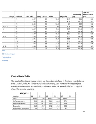
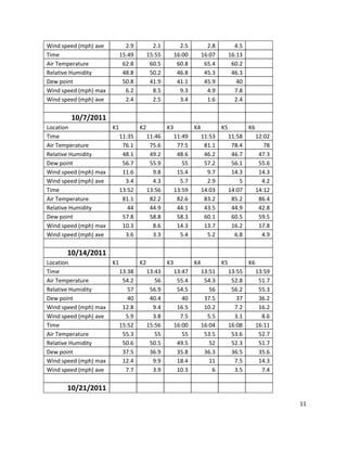
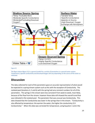
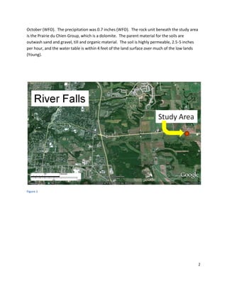
The document describes a study assessing water quality patterns in springs and a stream in River Falls, Wisconsin during fall 2011. 13 fixed sampling locations were established at 3 springs and various points upstream and downstream in the stream. Water quality parameters including temperature, dissolved oxygen, conductivity, and specific conductance were measured weekly from September to October using YSI instruments. Air temperature, humidity, wind speed and other weather data were also collected using a Kestrel meter. The results of these measurements are displayed in tables. The goal was to determine how spring discharge affects these field water quality parameters in the stream.
![6
Methodology
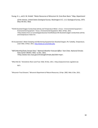
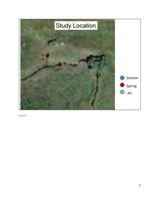
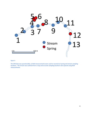
There were 13 fixed Spring and Stream locations in the South Fork (Figure 2 and 3). There was
one location at each of the three Springs. One location was located both 50 and 100 feet
downstream from each of the springs. One location was located 50 feet upstream from each of
the springs. The locations both upstream and downstream from the isolated pool were
measured from the nearest bank at the confluence of the pool and the South Fork. An
additional location was added on the right bank of the South Fork just past the confluence. All
distances were measured along the South Fork. Two additional points were located in the
isolated pool, one Northeast and one South of the Spring. Measurments were not taken due to
safety concerns about the instability of the ground in the isolated pool. 49 feet separated the
confluence and location 8, the second Spring. One location was taken at the half way point,
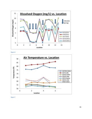
24.5 feet. Location 5, 8 and 12 were Spring locations. Location 4, 5 and 6 were in the isolated
pool. Locations 1, 2, 3,7,9,10,11, and 13 were the Stream locations. The data was collected
every Friday from September 16th until October 21st. The time the data was collected varied
slightly, however all data was collected between 11:00 a.m. and 6:00 p.m. The instruments
that were used for this study are the YSI-85, YSI-2030, Kestrel 3000 and the Garmin GPS 60. The
YSI-85 and the YSI-2030 are both water sampling and monitoring meters. The Kestrel 3000 is a
wind meter. The Garmin GPS 60 is a global positioning system used to collect accurate location.
Kestrel measurements were taken before and after the water (YSI) measurements each day.
The measurements were taken 6 feet above the water at locations 1, 2 and 4; a closer proximity
to the Stream. They were taken 6 feet above the land at locations 3, 5 and 6; a farther
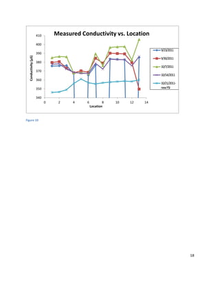
proximity from the Stream. The measurement parameters for the YSI instruments were: Water
Temperature (Celsius), Dissolved Oxygen (%), Dissolved Oxygen (mg/L), Conductivity (micro
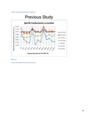
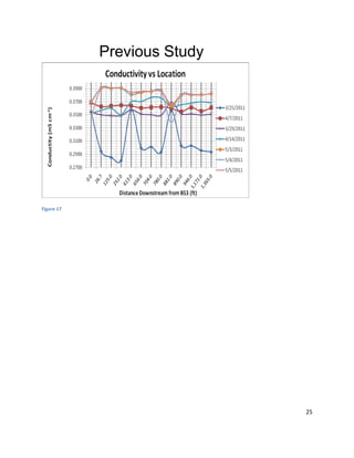
Siemens)(µS) and Specific Conductance (micro Siemens)(µS). “Conductivity is the ability of a
material to conduct electrical current” (YSI Incorporated). “Cell geometry affects conductivity
values, standardized measurements are expressed in specific conductivity units (S/cm) to
compensate for variations in electrode dimensions” (YSI Incorporated). The parameters for the
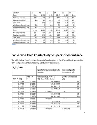
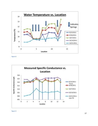
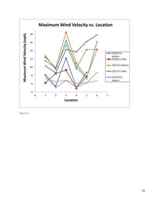
Kestrel 3000 are Air Temperature (Celsius), Relative Humidity, Dew point, Maximum wind
velocity (mph) and Average wind velocity (mph). There were several equations used in this
study. A Speific conductance formula, Equation 1, [Specific Conductance (25°C) =
Conductivity/(1 + TC * (T - 25))], was used for quality. The variables for this equation are: T=
Temperature and TC=0.0191. “Unless the solution being measured consists of pure KCl in
water, this temperature compensated value will be somewhat inaccurate, but the equation
with a value of TC = 0.0191 will provide a close approximation for solutions of many common
salts such as NaCl and NH4Cl and for seawater” (YSI 85). This equation, Equation 1, was also
algebraically manipulated to solve for Conductivity, Equation 2. The measured results were](https://image.slidesharecdn.com/feaebc7a-0c11-4bfb-8b0d-9f4d9646fa10-150611203453-lva1-app6892/85/SeniorResearch-6-320.jpg)
![7
compared to the results from the equation. An equation was also used to solve for Celsius
using Fahrenheit as the input, Equation 3, [Celsius= (5/9)*(Fahrenheit-32)].
.
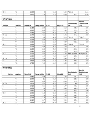
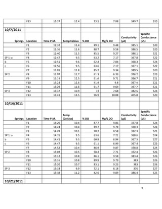
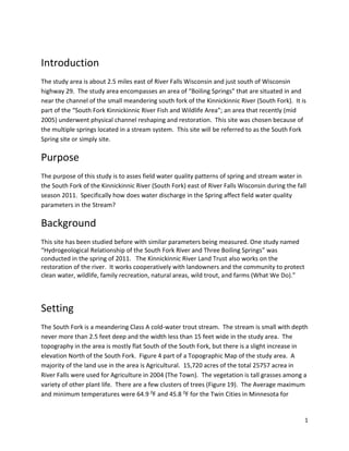
Results
YSI Data Table
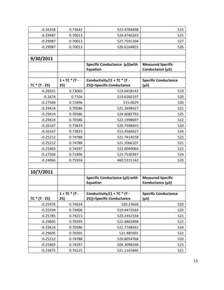
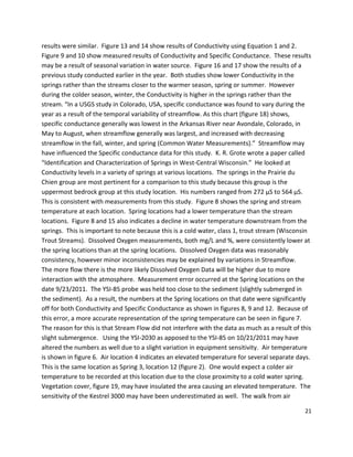
The results of the YSI measurements are shown below in Table 1. The items recorded were
Date, Spring locations, all locations, Time, Temperature, Dissolved Oxygen (both Percent and
milligrams per liter), Conductivity and Specific Conductance. Additional locations were added
after week 1, 9/16/2011. The week of 9/23/2011 there was disturbance in the water at Spring
1 (locations 4, 5 and 6). Duplicate samples were taken to provide quality control. Springs are
indicated by SP and a, b, and c following SP 1 (Isolated pool) indicated the sampling locations.
Point “a” is South of the Spring, “b” is at the Spring and “c” is Northeast of the Spring. Figure 2
and 3 show the sampling locations.
9/16/2011
Springs Location Time P.M.
Temp.
Celsius % DO Mg/L DO
Conductivity
(µS)
*Specific
Conductance
(µS)
F1 12:28 10.3 71.6 7.78 373.2 0.37
F2 12:42 10.2 69.2 7.53 372.9 0.37
F3 12:46 10.3 73.9 8.26 373.5 0.37
SP 1 F4 12:51 9 48.4 5.61 *100.9 0.1
F5 12:56 10.4 72.9 8.11 374.8 0.37
SP 2 F6 13:02 9 46.8 5.4 *120.2 0.12
F7 13:23 10.9 76.2 8.35 380.1 0.38
F8 13:28 10.9 75.1 8.3 380.3 0.38
F9 13:35 10.9 73.6 8.14 380.5 0.38](https://image.slidesharecdn.com/feaebc7a-0c11-4bfb-8b0d-9f4d9646fa10-150611203453-lva1-app6892/85/SeniorResearch-7-320.jpg)