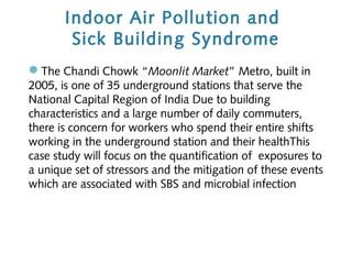
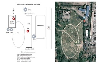
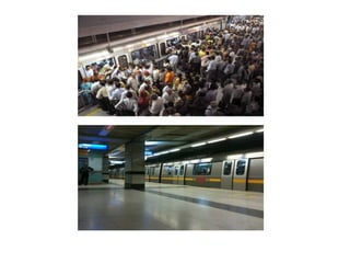
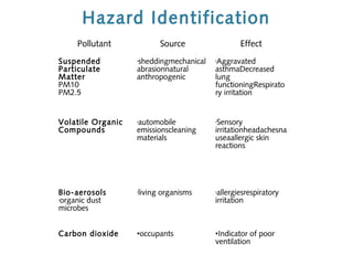
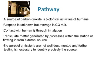
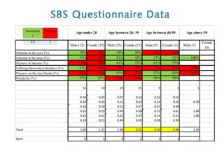
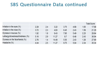
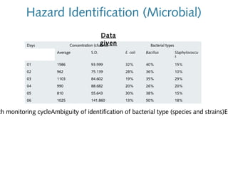
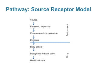
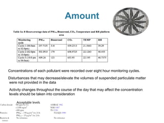
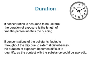
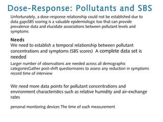
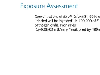
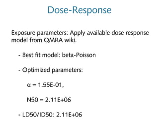
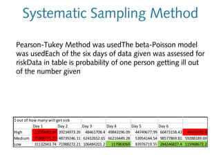
1) The document presents a case study analyzing indoor air pollution and sick building syndrome (SBS) in the underground Chandi Chowk metro station in New Delhi, India. 2) It identifies various air pollutants like particulate matter, volatile organic compounds, bioaerosols, and carbon dioxide that could be contributing to SBS. Questionnaires were used to assess SBS symptoms in station workers. 3) Exposure to the pollutants was assessed by measuring their concentrations over time, identifying sources, inhalation pathways, and establishing dose-response relationships between pollutant levels and SBS symptoms. More data is needed to better understand these relationships.

1. Air Pollutants and Health Risks:
A Case Study of Sick Building Syndrome
(SBS) in an Underground Metro Station
Platform Area in Tropical Region
Lee Voth-Gaeddert
Yiseul Kim
David Melton
Stephanie Stumpos
Mentors: Dr. Mukesh Khare & Dr. Hernando Perez

2. Indoor Air Pollution and
Sick Building Syndrome
—The Chandi Chowk “Moonlit Market” Metro, built in
2005, is one of 35 underground stations that serve the
National Capital Region of India Due to building
characteristics and a large number of daily commuters,
there is concern for workers who spend their entire shifts
working in the underground station and their healthThis
case study will focus on the quantification of exposures to
a unique set of stressors and the mitigation of these events
which are associated with SBS and microbial infection

5. Hazard Identification
Pollutant
Suspended
Particulate
Matter
PM10
PM2.5
Volatile Organic
Compounds
Bio-aerosols
•organic dust
microbes
Carbon dioxide
Source
sheddingmechanical
abrasionnatural
anthropogenic
•
automobile
emissionscleaning
materials
•
living organisms
Effect
Aggravated
asthmaDecreased
lung
functioningRespirato
ry irritation
•
Sensory
irritationheadachesna
useaallergic skin
reactions
•
allergiesrespiratory
irritation
•
•
•occupants
•Indicator of poor
ventilation

6. Exposure Assessment: Pollutants
Sick Building Syndrome is a discomfort caused by poor
air quality, and only exists while the sufferer inhabits the
building or container in question.

7. Exposure Assessment: Pollutants
In contrast to microbial infection, sick building syndrome
exists only while the sufferer inhabits the container of interest.
This suggests that the substance of interest is not a microbial
but rather a chemical hazard.

8. Exposure Assessment Tasks
Pathway
Amount
Duration

9. Pathway: Source Receptor Model

10. Pathway
•
A source of carbon dioxide is biological activities of humans
•
Airspeed is unknown but average is 0.3 m/s.
•
Contact with human is through inhalation
Particulate matter generated by processes within the station or
flowing in from external source
•
•
Bio-aerosol emissions are not well documented and further
testing is necessary to identify precisely the source

11. Amount
Concentrations of each pollutant were recorded over eight hour monitoring cycles.
Disturbances that may decrease/elevate the volumes of suspended particulate matter
were not provided in the data
Activity changes throughout the course of the day that may affect the concentration
levels should be taken into consideration
Acceptable levels

12. Duration
If concentration is assumed to be uniform,
the duration of exposure is the length of
time the person inhabits the building.
•
If concentrations of the pollutants fluctuate
throughout the day due to external disturbances,
the duration of exposure becomes difficult to
quantify, as the contact with the substance could be sporadic.
•

13. Dose-Response: Pollutants and SBS
Unfortunately, a dose-response relationship could not be established due to
data gapsSBS scoring is a valuable epidemiologic too that can provide
prevalence data and elucidate associations between pollutant levels and
symptoms
Needs
We need to establish a temporal relationship between pollutant
concentrations and symptoms (SBS scores) A complete data set is
needed
Larger number of observations are needed across all demographic
categoriesGather post-shift questionnaires to assess any reduction in symptoms
record time of interview
We need more data points for pollutant concentrations and
environment characteristics such as relative humidity and air-exchange
rates
personal monitoring devices The time of each measurement

14. SBS Questionnaire Data
Sometime
s
Always
0.5
1
Age under 20
Age between 20- 39
Age between 40-59
Male (12) Female (10) Male (23) Female (15)
Male (9)
Age above 59
Female (3)
Female
(0)
Male (1)
19%
31%
16%
43%
23%
37%
24%
23%
18%
29%
14%
25%
14%
21%
41%
49%
63%
49%
25%
43%
53%
58%
37%
65%
52%
27%
61%
72%
27%
56%
55%
52%
75%
81%
42%
78%
100%
100%
100%
-
12
10
23
15
9
3
1
0.10
0.16
0.16
0.22
0.23
0.19
0.24
0.23
0.18
0.29
0.14
0.13
0.07
0.11
0.21
0.49
0.32
0.49
0.13
0.22
0.27
0.58
0.37
0.65
0.52
0.14
0.31
0.72
0.14
0.28
0.55
0.26
0.38
0.81
0.21
0.39
Total
1.04
1.21
1.68
2.21
2.10
2.60
2.50
Rank
6
5
4
2
3
1
-
Irritation in the eyes (%)
Irritation in the nose (%)
Dryness in mucous (%)
Lethargy/drowsiness/tiredness (%)
Dryness on the face/hands (%)
Headache (%)
0.50
1.00
1.00

15. SBS Questionnaire Data continued

16. Hazard Identification (Microbial)
Data
given
Concentration (cfu/m3)
Days
Bacterial types
Average
S.D.
E. coli
Bacillus
Staphylococcu
s
01
1586
93.599
32%
40%
15%
02
962
75.139
28%
36%
10%
03
1103
84.602
19%
35%
29%
04
990
88.682
20%
26%
20%
05
810
55.643
30%
38%
15%
06
1025
141.860
13%
50%
18%
ch monitoring cycleAmbiguity of identification of bacterial type (species and strains)Ex

17. Escherichia coli (E. coli)
A large and diverse group of bacteriaGram-negative,
facultative anaerobic, and rod-shaped Commonly found in
the lower intestine of warm-blooded organismsUsed as
markers for water contaminationMost strains of E. coli are
harmless
Centers for Disease Control and Prevention

18. Escherichia coli (E. coli)
At present, 190 serogroups are known.Six pathotypes are
associated with diarrhea.
- Shiga toxin-producing E. coli (STEC)
- Enterotoxigenic E. coli (ETEC)
- Enteropathogenic E. coli (EPEC)
- Enteroaggregative E. coli (EAEC)
- Enteroinvasive E. coli (EIEC)
Centers for Disease Control and Prevention

19. Exposure Assessment
Concentrations of E.coli (cfu/m3): 50% o
inhaled will be ingested1 in 100,000 of E.
pathogenicInhalation rates
(u=5.0E-03 m3/min) *multiplied by 480m

20. Dose-Response
Exposure parameters: Apply available dose response
model from QMRA wiki.
- Best fit model: beta-Poisson
- Optimized parameters:
α = 1.55E-01,
N50 = 2.11E+06
- LD50/ID50: 2.11E+06

21. Pearson-Tukey Method
—Decision Tree model basedAllows analysis of three
different scenarios;
μ+
1
.6
4Ϭ
—BestWorstAverage
μ-1
.6
μ
4Ϭ
Best
Average
Worst

22. Tukey Test
Day 1
Day 2
Day 3
Day 4
Day 5
Day 6
High
594.8751008 334.1625188 270.540551 263.0420656 292.9821591 216.8045679
Medium
508
269
210
198
243
133
Low
421.1248992 182.1248992 123.1248992 111.1248992 156.1248992 46.1248992
1/100,000 chance of pathogic e coli
cfu/m3
Day 1
Day 2
Day 3
Day 4
Day 5
Day 6
High
0.005948751 0.003341625 0.002705406 0.002630421 0.002929822 0.002168046
Medium
0.00508
0.00269
0.0021
0.00198
0.00243
0.00133
Low
0.004211249 0.001821249 0.001231249 0.001111249 0.001561249 0.000461249
50% of microbes inhaled will be ingested
cfu/m3
Day 1
Day 2
Day 3
Day 4
Day 5
Day 6
High
0.002974376 0.001670813 0.001352703 0.00131521 0.001464911 0.001084023
Medium
0.00254 0.001345
0.00105
0.00099
0.001215
0.000665
Low
0.002105624 0.000910624 0.000615624 0.000555624 0.000780624 0.000230624
Taking into account breathing rate of 2.4 m3/8hrs
shift = 8 hours
Day 1
Day 2
Day 3
Day 4
Day 5
Day 6
High
0.007138501 0.00400995 0.003246487 0.003156505 0.003515786 0.002601655
Medium
0.006096 0.003228
0.00252
0.002376
0.002916
0.001596
Low
0.005053499 0.002185499 0.001477499 0.001333499 0.001873499 0.000553499

23. Systematic Sampling Method
Pearson-Tukey Method was usedThe beta-Poisson model
was usedEach of the six days of data given was assessed for
riskData in table is probability of one person getting ill out
of the number given
1 out of how many will get sick
Day 1
Day 2
Day 3
Day 4
Day 5
Day 6
High
22039682.64 39234973.26 48461708.4 49843196.09 44749677.99 60473158.43 44133732.8
Medium 25808775.77 48739246.11 62432652.65 66216449.28 53954144.54 98577869.81 59288189.69
Low
31132943.74 71988272.21 106484201.2 117983069 83976719.55 284246827.4 115968672.2

24. Risk Management
—ASHRAE Ventilation standards
—Between 15 and 60 cubic ft./m of outdoor air per personFiltration
devices; increased air exchangeInstallation of monitoring systems
Conducting emission inventory Cost benefit analysis: compare
productivity lost to sick days and the cost of improvements to station

25. Risk Communication
Employer
Employer
Regulatory agencies
Employee

26. References
Abdul-Wahab, Sabah A. Sick Building Syndrome: In Public Buildings and Workplaces. Berlin: Springer, 2011. Internet
resource.
Apte, Michael G, William J. Fisk, and Joan M. Daisey. Associations between Indoor Co2 Concentrations and Sick
Building Syndrome Symptoms in Us Office Buildings: An Analysis of the 1994-1996 Base Study Data. Berkeley, CA:
Lawrence Berkeley National Laboratory, 2000. Print.
Dybwad, Marius, Gunnar Skogan, and Janet Martha Blatny. ''Temporal Variability of the Bioaerosol Background at a
Subway Station: Concentration 2 Level, Size Distribution and Diversity of Airborne Bacteria. American Society for
Microbiology, 2013.
Exposure Factors Handbook. Washington, DC: Exposure Assessment Group, Office of Health and Environmental
Assessment, U.S. Environmental Protection Agency, 1989. Print.
Gupta, S, M Khare, and R Goyal. "Sick Building Syndrome-a Case Study in a Multistory Centrally Air-Conditioned
Building in the Delhi City." Building and Environment. 42.8 (2007): 2797-2809. Print.
Indoor Air Facts, No. 4: Sick Building Syndrome. Washington, D.C: U.S. Environmental Protection Agency, Office of Air
and Radiation, 1991. Print.

27. Chart Reference