Download to read offline
![SORT BENCHMARK 2014 1
DeepSort: Scalable Sorting with High Efficiency
Zheng Li1 and Juhan Lee2
Abstract—We have designed a distributed sorting engine opti-mized
for scalability and efficiency. In this report, we present the
results for the following sort benchmarks: 1) Indy Gray Sort and
Daytona Gray Sort; 2) Indy Minute Sort and Daytona Minute
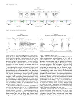
Sort. The submitted benchmark results are highlighted in Table I.
I. INTRODUCTION
DeepSort is a salable and efficiency-optimized distributed
general sorting engine. We engineered the software design for
high performance based on the two major design decisions:
Parallelism at all sorting phases and components is max-imized
through properly exposing program concurrency
to thousands of user-level light-weight threads. As a
result, computation, communication, and storage tasks
could be highly overlapped with low switching overhead.
For instance, since hard drives are optimal for sequential
access, the concurrency of storage access is limited while
computation and communication threads are overlapped
to take advantage of remaining resources. We use Go
language to orchestra the massive parallel light-weight
threads, i.e. Go routines. Individual sorting functions are
implemented in C for high performance.
Data movements in both hard drives and memories are
minimized through an optimized data flow design that
maximizes memory and cache usage. Specifically, we
avoid using disks for data buffering as much as possible.
For data buffered in memory, we separate key data that
need frequent manipulation from payload data that are
mostly still. In this way, performance could be improved
through minimal data movements for payloads and proper
caching on the frequently accessed keys.
We have deployed DeepSort in a cluster with approximately
400 nodes. Each node has two 2.1GHz Intel Xeon hexa-core
processors with 64GB memory, eight 7200rpm hard drives,
and one 10Gbps Ethernet port. These servers are connected
in a fat-tree network with 1.28:1 TOR to spine subscription
ratio. We equipped these servers with CentOS 6.4 and ext4
file systems. We’ve carefully measured the performance of
DeepSort on this platform based on Sort Benchmark FAQ [1]
for both Gray Sort and Minute Sort. The submitted benchmark
results are highlighted in Table I.
In this rest of the report, we explain the software design of
DeepSort in Section II. The underlying hardware and operation
system platforms are described in Section III, followed by the
the detailed experiment measurements in Section IV.
Contact: zheng.l@samsung.com
1. Research Engineer, Cloud Research Lab, Samsung Research America
Silicon Valley, San Jose, CA U.S.
2. Vice President, Intelligence Solution Team, Samsung Software RD
Center, Korea
II. DESIGN OF DEEPSORT
The design of DeepSort targets high efficiency at a large
scale. To reach this goal, we designed a fluent data flow that
shares the limited memory space and minimizes data move-ment.
We also express data processing concurrency through
light weight threading and optimize parallelism at all stages
and components of the program. This section explains the
implementation of such design philosophy and specific design
choices in the distributed external sorting program.
A. Design Overview
The overall design has been depicted in Figure 1 from the
perspective of records to be sorted. A record is first fetched
from the source disk to the memory, sorted and distributed
to the destination node, merged with other records based on
order, and finally written to the destination disk. For cases
like Gray Sort, in which the amount of the data is larger
than the aggregated capacity of memory, multiple rounds of
intermediate sorts are executed. The final round merges spilled
intermediate data from previous rounds. The input of the
un-sorted records are distributed evenly across nodes, and
the output are also distributed based on key partitions. The
concatenated output files are formed into a globally sorted list.
RAID-6 erasure coding across nodes is used for replication in
Daytona sort 1. The data read procedure includes detecting
possible failures and recovering data from erasure decoding.
The data write procedure is followed by sending data to other
nodes for erasure encoding.
Each process phase in Figure 1 is described below from
source disks to destination disks. A table of notations is
presented in Table II for ease of understanding. We leverage
both data parallelism and task parallelism to exploit the con-currency
in the distributed sorting. There is only one process
per node with thousands of light weight threads to handle
different functionalities concurrently. To illustrate the abundant
parallelism, we count the number of light weight threads as in
Table III. The light weight threading library, i.e. Go runtime,
multiplexes them onto OS threads for high performance. Mem-ory
is shared among these threads to minimize IO operations
and thus optimize the overall performance. As we maximize
the memory usage by sharing the same address space, only
pointers are passed between different phases except across
nodes or rounds.
A record is first fetched from a source disk by a reader
thread. One reader thread is assigned to each hard drive to
guarantee the sequential access of disks. Data are fetched from
disk consecutively. They are divided evenly into R rounds and
each round has B batches. For Daytona sort, batch is also the
erasure coding granularity, i.e. size of coding block. Once a
1Based on email communications with the SortBenchmark committee, such
replication complies with the competition rules.](https://image.slidesharecdn.com/deepsort2014-141127083411-conversion-gate01/85/Samsung-DeepSort-1-320.jpg)
![SORT BENCHMARK 2014 1
DeepSort: Scalable Sorting with High Efficiency
Zheng Li1 and Juhan Lee2
Abstract—We have designed a distributed sorting engine opti-mized
for scalability and efficiency. In this report, we present the
results for the following sort benchmarks: 1) Indy Gray Sort and
Daytona Gray Sort; 2) Indy Minute Sort and Daytona Minute
Sort. The submitted benchmark results are highlighted in Table I.
I. INTRODUCTION
DeepSort is a salable and efficiency-optimized distributed
general sorting engine. We engineered the software design for
high performance based on the two major design decisions:
Parallelism at all sorting phases and components is max-imized
through properly exposing program concurrency
to thousands of user-level light-weight threads. As a
result, computation, communication, and storage tasks
could be highly overlapped with low switching overhead.
For instance, since hard drives are optimal for sequential
access, the concurrency of storage access is limited while
computation and communication threads are overlapped
to take advantage of remaining resources. We use Go
language to orchestra the massive parallel light-weight
threads, i.e. Go routines. Individual sorting functions are
implemented in C for high performance.
Data movements in both hard drives and memories are
minimized through an optimized data flow design that
maximizes memory and cache usage. Specifically, we
avoid using disks for data buffering as much as possible.
For data buffered in memory, we separate key data that
need frequent manipulation from payload data that are
mostly still. In this way, performance could be improved
through minimal data movements for payloads and proper
caching on the frequently accessed keys.
We have deployed DeepSort in a cluster with approximately
400 nodes. Each node has two 2.1GHz Intel Xeon hexa-core
processors with 64GB memory, eight 7200rpm hard drives,
and one 10Gbps Ethernet port. These servers are connected
in a fat-tree network with 1.28:1 TOR to spine subscription
ratio. We equipped these servers with CentOS 6.4 and ext4
file systems. We’ve carefully measured the performance of
DeepSort on this platform based on Sort Benchmark FAQ [1]
for both Gray Sort and Minute Sort. The submitted benchmark
results are highlighted in Table I.
In this rest of the report, we explain the software design of
DeepSort in Section II. The underlying hardware and operation
system platforms are described in Section III, followed by the
the detailed experiment measurements in Section IV.
Contact: zheng.l@samsung.com
1. Research Engineer, Cloud Research Lab, Samsung Research America
Silicon Valley, San Jose, CA U.S.
2. Vice President, Intelligence Solution Team, Samsung Software RD
Center, Korea
II. DESIGN OF DEEPSORT
The design of DeepSort targets high efficiency at a large
scale. To reach this goal, we designed a fluent data flow that
shares the limited memory space and minimizes data move-ment.
We also express data processing concurrency through
light weight threading and optimize parallelism at all stages
and components of the program. This section explains the
implementation of such design philosophy and specific design
choices in the distributed external sorting program.
A. Design Overview
The overall design has been depicted in Figure 1 from the
perspective of records to be sorted. A record is first fetched
from the source disk to the memory, sorted and distributed
to the destination node, merged with other records based on
order, and finally written to the destination disk. For cases
like Gray Sort, in which the amount of the data is larger
than the aggregated capacity of memory, multiple rounds of
intermediate sorts are executed. The final round merges spilled
intermediate data from previous rounds. The input of the
un-sorted records are distributed evenly across nodes, and
the output are also distributed based on key partitions. The
concatenated output files are formed into a globally sorted list.
RAID-6 erasure coding across nodes is used for replication in
Daytona sort 1. The data read procedure includes detecting
possible failures and recovering data from erasure decoding.
The data write procedure is followed by sending data to other
nodes for erasure encoding.
Each process phase in Figure 1 is described below from
source disks to destination disks. A table of notations is
presented in Table II for ease of understanding. We leverage
both data parallelism and task parallelism to exploit the con-currency
in the distributed sorting. There is only one process
per node with thousands of light weight threads to handle
different functionalities concurrently. To illustrate the abundant
parallelism, we count the number of light weight threads as in
Table III. The light weight threading library, i.e. Go runtime,
multiplexes them onto OS threads for high performance. Mem-ory
is shared among these threads to minimize IO operations
and thus optimize the overall performance. As we maximize
the memory usage by sharing the same address space, only
pointers are passed between different phases except across
nodes or rounds.
A record is first fetched from a source disk by a reader
thread. One reader thread is assigned to each hard drive to
guarantee the sequential access of disks. Data are fetched from
disk consecutively. They are divided evenly into R rounds and
each round has B batches. For Daytona sort, batch is also the
erasure coding granularity, i.e. size of coding block. Once a
1Based on email communications with the SortBenchmark committee, such
replication complies with the competition rules.](https://image.slidesharecdn.com/deepsort2014-141127083411-conversion-gate01/75/Samsung-DeepSort-1-2048.jpg)
![SORT BENCHMARK 2014 3
does not fit into the aggregated memory, multiple rounds are
used. The write phase at the first R1 rounds spill the results
into sorted temporary files. Typically, writer threads generate
one file per round per disk. In extreme skewed cases where
the memory management thread notifies early second level
merging, multiple files are generated per round per disk. The
write phase at the last round merges temporary files generated
at all rounds with the final data received to form the output
sorted list. If replication is required as in Daytona sort, the
write phase will be followed by erasure encoding detailed in
Section II-F. Typically one final output file with optional codec
information is generated on each disk. The writing of output
files are overlapped with erasure encoding and corresponding
communication. For Indy Minute Sort, two output files with
separate key partition spaces are generated per disk so that
the writing of the first partition could be overlapped with the
communication of the second partition.
B. Partition
In parallel with the data path described above, the splitters
that determine the boundaries among nodes and disks are
computed so that the output could be almost evenly distributed
among all the disks. By evenly sampling data across all nodes
as late as possible with small performance interference, we
can cover a large portion of the data set. We use the following
algorithms to create a set of splitter keys targeting even output
partitions.
There are two levels of partitions, the first level determines
the key splitters among nodes in the cluster, i.e. node splitters,
and the second level determines the key splitters among disks
within a node, i.e. disk splitters. Both levels are variances of
sample splitting [2]. Unlike in-memory sorting, where splitters
could be gradually refined and data could be redistributed,
rebalancing in external sorting generally comes with high IO
overhead. Therefore, histogram splitting is not used.
The N 1 node splitters that partition key ranges among
nodes are determined in a centralized master node. Each node
is eligible to be a master node, but in case redundancy is
neeeded, master node could be picked by distributed leader
election algorithm. From all the nodes, after Bnode batches of
data are sorted, N 1 node splitter proposals are picked to
evenly partition the batch of data into N segments. These node
splitter proposals are aggregated to the master node. A total
of N D Bnode (N 1) proposals are then sorted in the
master node, and the final node splitters are determined by
equally dividing these proposals. Considering there might be
data skew, we over-sample the data s times by locally picking
Ns node splitter proposals that evenly partition the data into
N s segments. The final N 1 node splitters are thus picked
from a sorted listed of N DBnode N s proposals. This
process is carried in parallel with data read and sort, but before
the first round of sending data to its destinations to minimize
network overhead. We have describe the node splitter design
in Algorithm 1 and Algorithm 2.
The D 1 disk splitters per node are determined distribu-tively
at each destination node. After receiving data that equals
the size of Bdisk input batches from all peers, the destination
Algorithm 1 Partition among nodes: Proposals
Require: N, s, D, Bnode
1: procedure PROPOSAL(l) . A thread at each node
2: count = 0
3: while list l do . Pointer of sorted lists
4: len = length(list)
5: for i = 0:::N s 1 do
6: pos = len i=(N s 1)
7: Send list[pos]:Key
8: end for
9: count = count + 1
10: if count = D Bnode then
11: break . Sample threshold reached
12: end if
13: end while
14: Receive splitters . Final splitters from the master
15: end procedure
Algorithm 2 Partition among nodes: Decision
Require: N, s, D, Bnode
1: procedure DECISION . One thread in master
2: list = []
3: for i = 1:::N 2 D Bnode s do
4: Receive key
5: list = append(list; key)
6: end for
7: Sort(list) . Sort all keys received
8: for i = 1::N 1 do
9: pos = i length(list)=(N 1)
10: Broadcast list[pos]
11: end for
12: end procedure
node starts a separate thread that calculate the disk splitters
in parallel with receiver threads and merger threads. When
the disk splitter threads start, there are about Bdisk N D
sorted lists. For the i-th disk splitter, every sorted list proposes
a candidate. This candidate will be used to divide all the
other lists. The one that best approaches the expectation of
i-th splitter is picked as the final disk splitters. Unlike node
splitter algorithm, disk splitter algorithm is not on the critical
path of the program, and is carried in parallel with the first
level merging.
Comparing to existing external sort designs, we sample and
partition the key space in parallel with reading and sorting.
We also delay the disk partition as late as possible but
before second level merging. As shown in Table IV, DeepSort
achieves higher sampling coverage across all computing nodes
TABLE IV
EXTERNAL SORT SAMPLE COMPARISON
System Time of Sample Coverage rate Location
Hadoop [3] Before sorting 1=106 at most 10 nodes
TritonSort[4] Before sorting approx 1=1923 All nodes
DeepSort During sorting 1=50 All nodes](https://image.slidesharecdn.com/deepsort2014-141127083411-conversion-gate01/85/Samsung-DeepSort-3-320.jpg)
![SORT BENCHMARK 2014 4
in participation. As will be shown, DeepSort handles skewed
dataset much better than existing designs.
The cost of high sample rates only reveals in Daytona
Minute Sort. For Indy Sort, we set Bnode to 1 and s to 1
to minimize the time impact of partition. The partition takes
less than 2 seconds to complete at the master node. In order
to account for skewed data set, we set Bnode to 8 and s to
25 for Daytona Gray Sort. The node partition process takes
approximately 30 seconds to complete at the master node. This
has minimal impact of overall long sorting time but resulting
a reasonably balanced output. We set Bnode to 5 and s to 20 for
Daytona Minute Sort. The node partition takes approximately
more than 10 seconds to complete. This has a major impact
within a minute. The resulting Daytona Minute Sort data size
is only about 70% of the Indy Minute Sort. Unlike node
partition, disk partition is not in the execution critical paths
and does not cause extra run time.
C. Sort and Merge
Contrary to the rest of system, the individual sorting and
merging functions are implemented based on open source C
libraries, and we keep it general to any key and value sizes and
types. Comparison sort has been a well-studied topic. Instead
of examining the theoretical limits to pick the best algorithm,
we experiment with different designs and pick the best one in
practice.
For the individual local sort at the data source, we prefer in-place
sorting to minimize memory footprint. The performance
just needs to be higher than IO speed so that computation
latency could be hidden. Since the single disk hard drive
read speed is 150MB/s, for 100-byte record, the cut-off
performance is 1.5 million records per second. We picked the
QuickSort as the algorithm, and use the implementation of
GlibC qsort.
When hundreds and thousands of sorted list needs to be
merged, we use heap-sort to form a multi-way merging to
minimize memory foot print. Initially, a priority queue, i.e.
heap, is formed using the head of all sorted list. The merged
list is formed by extracting the head of the queue one by
one. Every extracted element is replaced by the head of the
corresponding input list. The property of priority queue is
kept during the process. Heap sort implementation is adopted
based on the heapsort in BSD LibC from Apple’s open source
site [5]. We keep its heapify macros for the implementation
efficiency, but revise the sort function to facilitate the multi-list
merge process. The algorithm is presented in Algorithm 3.
The performance of merging determines the merging threshold
m, i.e. the number of sorted list required to trigger a merging
thread. The last merging is accompanied with writing thread
should be faster than disk access speed to hide its latency. Our
experiments show that even over a thousand lists need to be
merged, the performance is still above the disk access speed.
We optimize the comparison operator to improve the per-formance
for comparison sort. In case string comparison is
used and the order is defined in memcmp, we convert byte
sequences into multiple 64-bit or 32-bit integers to minimize
the comparison instruction counts. Such optimization has
Algorithm 3 First-level premerger based on heap sort
Require: m, array, boundary, destination
1: procedure MERGE
2: heap []
3: for i = 1..m do . Initialize heap
4: heap[i].Key = array[boundary[i].Start]
5: heap[i].Position = boundary[i].Start
6: heap[i].Tail = boundary[i].End
7: end for
8: for i = m/2..1 do . Heapify
9: CREATE(i) . BSD LibC macro to build heap
10: end for
11: while heap not empty do
12: APPEND(destination, array[heap[1].Position])
13: heap[1].Position ++
14: if heap[1].Position==heap[1].Tail then
15: k heap[m]
16: m m 1
17: if m==0 then
18: break
19: end if
20: else
21: heap[1].Key = array[heap[1].Position]
22: k heap[1]
23: end if
24: SELECT(k) . BSD LibC macro to recover heap
25: end while
26: end procedure
shown moderate performance improvement. The comparison
operator could also be defined by users to accommodate
different sorting types or orders.
D. Communication
Like many of the cloud applications, distributed sorting
requires all-to-all reliable communication pattern. Therefore,
each of the node setups N1 sender and N1 receiver threads
for TCP/IP communication. Go runtime multiplexes these
lightweight threads onto system threads for communication.
Without such runtime management, setting up 2N 2 system
threads for communication scales poorly with N. Prior works
like TritionSort [4] or CloudRAM sort [6] uses one dedi-cate
communication thread to poll data from all computation
threads and distribute them to all destination. By leveraging
the Go runtime, we are able to implement highly salable
communication without additional code complexity.
To save the round-trip latency of data fetching, we adopt
push-based communication in which the data source side
initiate the transfer. The locally sorted lists are pushed to the
destination. We also prioritize key transfer over value transfer
so that the destination-side merging could start as early as
possible.
To avoid destination overflow in push-based communica-tion,
we orchestrate the communication using a light-load syn-chronization
mechanism between two rounds of data transfer.
After a node finishes writing temporary data of a round, it](https://image.slidesharecdn.com/deepsort2014-141127083411-conversion-gate01/85/Samsung-DeepSort-4-320.jpg)
![SORT BENCHMARK 2014 5
TABLE V
EXTERNAL SORT DATA BUFFERING COMPARISON
System # of movements in HDD # of movements in DRAM
Hadoop [3] 3 or 4 6
TritonSort[4] 2 5
DeepSort 2 4
10 Bytes 2 Bytes 4 Bytes
Keymsb Ld Pos
Data Length
Starting
Position
Example construction
Fig. 2. The pointer structure to link the key array to the data array
broadcasts one byte synchronization message to all the peers
notifying its progress. A node starts reading the input data
of the next round after local disk writes concludes but hold
the data transfer until it receives the synchronization messages
from all the peers. This light all-to-all synchronization is per-formed
during a relative idle period of network, and overlaps
with disk access and sorting.
E. Memory Management
The memory management design goal is to minimize data
movements for high performance and full utilization of re-sources.
As shown in Table V, DeepSort minimizes data
movements within hard drives and DRAM to minimal. Data
records in the last sorting round read and write hard drives
only once for input and output. The rest of records have one
more trip to hard drives for intermediate buffering due to the
fact that the aggregated memory size is smaller than overall
data size.
DeepSort also minimizes the segmentation of memory and
eliminates frequent movements of data within memory using
the efficient memory management mechanism. Although Go
language has its own mark-and-sweep garbage collection
mechanism, in practice it could not recover released memory
space immediately. Therefore, we manage the key and value
spaces ourselves while leaving trivial memory usage to Go
runtime.
DeepSort hosts two globally shared arrays that are persistent
and takes majority of available system physical memory.
The first array stores the data values, which are large but
infrequently access, and the second array stores the keys,
which are frequently accessed and altered, with corresponding
pointers to the data array. We refer to them as data array,
and key array, respectively. In this memory structure, the only
overhead per record is the pointers that link the key array to
data array. We have plotted the pointer from the key array to
the data array in Figure 2.
The pointer structure is parameterized to handle various key
and value sizes. It has three fields. An illustrative construction
is presented in Figure 2 and described as below.
1) Keymsb is the most important bytes of the key. Its size is
a fixed configuration parameter. Users could write custom
compare functions that further tap into the data array as
the extension of the key. This is made possible as the
whole structure is passed into sort and merge functions
and the data array is globally visible in a process. In the
example construction, we set the size to 10 bytes.
2) Ld represents the size of the payload data in terms of a
predefined block size Bs. The actual payload data size
is Bs (Ld + 1) bytes. For instance, we configure the
parameter Bs as 90 bytes and the width of Ld to two
bytes so that the variable payload size for each record
could be up to 5.9 MB. For fixed size 90-byte payload,
we can set Ld to 0.
3) Pos indicates the starting location of the data block.
Although the key array is frequently manipulated for
sorting, merging, and splitting, the data array doesn’t
move until records have been assembled for network
communication or disk accesses. At that time, the data
is assembled the same as the input format but with a
different order based on the key array.
For performance optimization, it is desirable to align the size
of the pointer structure to cache-line and memory access. In
the shown example, the structure size is 16 bytes.
The key array and data array are shared globally between
source sides and destination sides. They are working as
circular buffers. When sorted data from peers have arrived,
they are appended to the end of the array. When locally
sorted data have been released from the source, their space
is reclaimed. There is a dedicate thread that manages global
resources in parallel with other activities. To accommodate
the buffering behavior and moderate skewed data set, the
global arrays have auxiliary space that could be configured
depends on application. Once the auxiliary space is about to
be exhausted from receiving large amount of the extremely
skewed data, the memory management thread will notify the
second level merging threads to start spilling data to disks.
Space will be freed after spilling, and such mechanism might
iterate multiple times.
The memory layout is shown in Figure 3. Five snapshots
of the key array layout have been depicted, and the process is
explained as follows:
a) In the beginning of a round, the locally read data starts
filling the memory. There might be some leftovers from
previous round. All nodes synchronize with each other and
get ready for all-to-all communication.
b) In the middle of a round, more data has been read. The
initial batches of data has been sent out, and the space has
been freed. Data has been received from peers of this round,
and the memory gets filling up. The first-level mergers start
processing received sorted lists.
c) Towards the end of a typical round, after all local data has
been read, the disks are free to be written. The second-level
mergers start to merge and writers start spilling sorted lists.
If it is the last round, the spilling will wait until all data
has been received.](https://image.slidesharecdn.com/deepsort2014-141127083411-conversion-gate01/85/Samsung-DeepSort-5-320.jpg)
![SORT BENCHMARK 2014 6
Local read data
Freed space
Received data
Data being spilled
a) Round starts. Some data
read; some data from the
previous round
b) All local data read; Some
data sent; some data received
c) Merging and spilling data;
most data sent; most data
received
d) Spilled data free up space;
Finish the remaining send and
receive
e) All data sent and received;
remaining data for next round
Fig. 3. Snapshots of memory layouts as a circular buffer.
d) Towards the end of a extremely skewed round, data is
being received to fill the full memory space. Memory
management thread notifies second-level mergers to spill
data out to free space.
e) At the end of a round, all current round data have been
received and sent. If the round is not the last, there might
be leftovers for the next round.
F. Replication Strategy
We use erasure code to protect data failures across nodes.
As an optional feature of DeepSort, replication could be turned
on to protect data failures of up to two nodes in Daytona Sort.
It could also be turned off for better performance in Indy Sort.
Replication only apply to input and output data, and it does
not apply to intermediate data.
Specifically, we use Minimal Density RAID-6 Coding
across nodes. This is a Maximum Distance Separable (MDS)
codes. For every k nodes that hold input and output data, we
use extra m nodes to hold codes that are calculated from the
original k nodes. Since it is a MDS code, the system is able
to tolerate any m nodes loss. We divided all nodes n into
n=k k-node groups in a circle. The calculated m codes from
each group are evenly distributed in the k nodes of the next
group. In Figure 4, we show an illustration of data layout for
a total of 6 nodes with k equaling 3 and m equaling 2. Using
RAID-6 coding, we can trade-off between disk bandwidth and
computation resources without sacrificing the data replication
rate. In our Daytona sort experiments, we set k equals 8 and
m equals 2. Therefore, it could tolerate at most 2-node failures
and the extra disk bandwidth required for replication is only
25% of the data size.
For encoding and decoding, our implementation uses Jera-sure
erasure coding library from University of Tennesse [7].
Codec has been embedded in our sorting pipeline. Decoding
is part of data read. If any node loss or data corruption
detected, data has to be pulled from multiple nodes to recover
missing data. In case of no loss, the decoding is simplified as
a direct read from data hard drives. Encoding is embedded in
final data write. We have completely overlap the computation,
communication, and disk access for the write replication
process. Figure 5 illustrates such pipeline.
Encoding process is depicted in Figure 5. On the destination
side of DeepSort, the process starts after initial sorted data has
been merged and assembled in the pipeline. While the sorted
data is being committed into hard drives, they are also being
sent to major encoding nodes in the next k-node group. For
Node 0 Node 1 Node 2 Node 3 Node 4 Node 5
Group 0 Group 1
Data 0
Data 1
Data 2
Code 0
Code 1
Code 2
Major Minor
data blocks m=3 code blocks k=2
Legend:
Fig. 4. Illustration of data layout for replication
Merging data
Write data to local
disks
Send data to a round-robin
node in the next
group
Minor Coding Major Coding Node Data node
Node
Erasure coding
data
Write local part
of the code
Send remote
part of the code
Write code
Written data synchronized with disks
Fig. 5. Data pipeline of erasure coding](https://image.slidesharecdn.com/deepsort2014-141127083411-conversion-gate01/85/Samsung-DeepSort-6-320.jpg)

![SORT BENCHMARK 2014 9
TABLE XI
DAYTONA MINUTE SORT SKEW
Amount of Data 3686.4 GB
Duplicate Keys 66369138
Input Checksum 44aa2f5711f86b65f
Trial 1 1 min 33.686 sec
Trial 2 1 min 23.333 sec
Trial 3 1 min 33.077 sec
Trial 4 1 min 51.229 sec
Trial 5 1 min 25.131 sec
Trial 6 1 min 30.805 sec
Trial 7 1 min 27.761 sec
Trial 8 1 min 33.522 sec
Trial 9 1 min 33.351 sec
Trial 10 1 min 24.555 sec
Trial 11 1 min 31.157 sec
Trial 12 1 min 28.696 sec
Trial 13 1 min 27.028 sec
Trial 14 1 min 26.570 sec
Trial 15 1 min 31.841 sec
Trial 16 1 min 33.769 sec
Trial 17 1 min 39.421 sec
Output checksum 44aa2f5711f86b65f
Median time 1 min 31.157 sec
TABLE X
DAYTONA MINUTE SORT RANDOM
Amount of Data 3686.4 GB
Duplicate Keys 0
Input Checksum 44aa164cc14340759
Trial 1 0 min 57.299 sec
Trial 2 0 min 55.581 sec
Trial 3 0 min 59.408 sec
Trial 4 0 min 57.675 sec
Trial 5 0 min 59.146 sec
Trial 6 0 min 56.590 sec
Trial 7 0 min 55.557 sec
Trial 8 0 min 57.937 sec
Trial 9 0 min 59.300 sec
Trial 10 0 min 57.017 sec
Trial 11 0 min 59.858 sec
Trial 12 0 min 51.672 sec
Trial 13 0 min 59.145 sec
Trial 14 1 min 1.159 sec
Trial 15 0 min 59.053 sec
Trial 16 0 min 56.647 sec
Trail 17 0 min 54.610 sec
Output checksum 44aa164cc14340759
Median time 0 min 57.675 sec
E. Minute Sort Daytona Results
For the Daytona variant of Minute Sort, we sorted 3686.4GB
random data in 57.675 seconds which is the median time of
17 consecutive runs. The sorting time for skewed data is less
than twice of the random data.
Specifically, we use 384 nodes of the cluster. Each
node hosts 9.6GB input data. The input checksum is
44aa164cc14340759 without duplications. We’ve sorted this
data in seventeen consecutive runs, and the running time
reported by time utility are listed in Table X. The outputcheck-sum
is also 44aa164cc14340759. There is no intermediate data
for Minute Sort.
We also prepared skewed dataset and run DeepSort using
384 nodes of the cluster, totaling 3686.4 GB of skewed data
with a checksum of 44aa2f5711f86b65f. There are 66369138
duplicate keys in the input. We’ve also sorted the skewed data
in seventeen consecutive runs, and the running time reported
by time utility are listed in Table XI. The output checksums
are also 44aa2f5711f86b65f, and the median sorting time is
91.157 seconds, which is less than twice of the random input
sorting time.
V. ACKNOWLEDGMENT
DeepSort results are made possible with the strong support
of all members in the Cloud Research Lab of Samsung Re-search
America, Silicon Valley. Specifically, Lohit Giri, Venko
Gospodinov, Hars Vardhan, and Navin Kumar have helped
with the infrastructure provision. Minsuk Song, Jeehoon Park,
Jeongsik In, and Zhan Zhang have helped with the network-ing.
Hadar Isaac and Guangdeng Liao have advised on the
sorting design. We would like to appreciate Sort Benchmark
committee members (Chris Nyberg, Mehul Shah, and Naga
Govindaraju) for valuable comments.
REFERENCES
[1] C. Nyberg, M. Shah, and N. Govindaraju, “Sort FAQ (14 March 2014),”
http://sortbenchmark.org/FAQ-2014.html, 2014, [Online].
[2] J. Huang and Y. Chow, “Parallel sorting and data partitioning by
sampling,” in IEEE Computer Society’s Seventh International Computer
Software and Applications Conference (COMPSAC’83), 1983, pp. 627–
631.
[3] T. Graves, “GraySort and MinuteSort at Yahoo on Hadoop 0.23,” http:
//sortbenchmark.org/Yahoo2013Sort.pdf, 2013.
[4] A. Rasmussen, G. Porter, M. Conley et al., “Tritonsort: A balanced large-scale
sorting system,” in Proceedings of the 8th USENIX conference on
Networked systems design and implementation, 2011, p. 3.
[5] “Heap sort,” http://www.opensource.apple.com/source/Libc/Libc-167/
stdlib.subproj/heapsort.c, 1999, [Online].
[6] C. Kim, J. Park, N. Satish et al., “CloudRAMSort: fast and efficient large-scale
distributed RAM sort on shared-nothing cluster,” in Proceedings of
the 2012 ACM SIGMOD International Conference on Management of
Data, 2012, pp. 841–850.
[7] J. S. Plank and K. M. Greenan, “Jerasure: A library in C facilitating
erasure coding for storage applications – version 2.0,” University of
Tennessee, Tech. Rep. UT-EECS-14-721, January 2014.](https://image.slidesharecdn.com/deepsort2014-141127083411-conversion-gate01/85/Samsung-DeepSort-9-320.jpg)

The document describes Deepsort, a scalable and efficient distributed sorting engine optimized for performance through parallelism and minimized data movement. Deepsort is implemented on a 400-node cluster and leverages lightweight threading and optimized data processing to enhance sorting capabilities across large datasets. Benchmark results demonstrate its effectiveness in handling gray sort and minute sort tasks with significant throughput improvements compared to existing sorting solutions.


![Getting Started with Apache Spark: Big Data Made Simple [Free Meetup]](https://cdn.slidesharecdn.com/ss_thumbnails/apachesparkgettingstarted-260203175547-8361bcc3-thumbnail.jpg?width=640&height=640&fit=bounds)


