Download to read offline

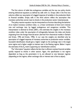
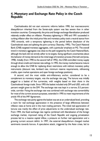
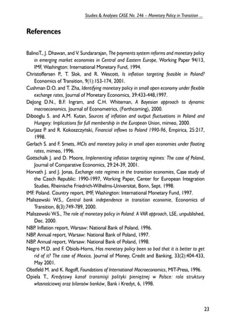
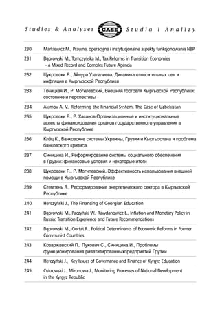
![Appendix A. Data sources and transformations
Money market rates:
Czech Republic: 1 month PRIBOR – Czech National Bank
Poland: 1 month WIBOR – Datastream
Exchange rate indices:
Czech Republic: (0.35 log(CZK/USD) + 0.65 log(CZK/DM)) – Czech National
Bank
Poland: (0.5 log(PLN/USD) + 0.5 log(PLN/DM)) – National Bank of Poland
Consumer Price Indices CPI (log of X11 seasonally adjusted series)
Czech Republic: Czech National Bank
Poland – Central Statistical Office
Index of Industrial Production IIP (log of X11 seasonally adjusted series)
Czech Republic: Czech National Bank
Poland: Central Statistical Office
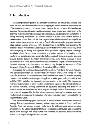
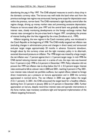
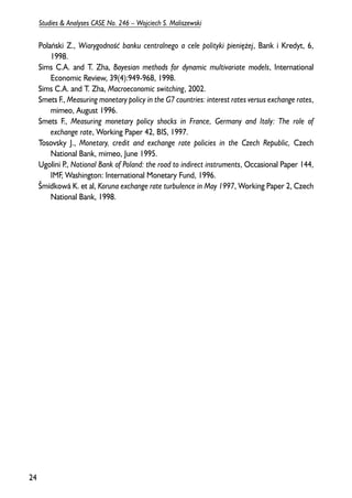
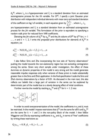
Appendix B. Bayesian estimation
The estimation method for the multi-regime model in this paper is adapted from Del
Negro and Obiols-Homs (2001) (who estimate a similar model for Mexico) and Sims and
Zha (2002). The following description follows closely Sims and Zha but is simplified due
to my assumption that dates of regime changes are known.
Following Sims and Zha, I begin by rewriting the model 1 in the following way
(1)
’
ytA = x [D + SA ]+ ε
where
(2)
=
nxn
0
I specify priors for non-zero coefficients in A0 (for regimes k=1,2) in the same way as
in Sims and Zha (2002), assuming a joint Gaussian prior distribution with independent
individual elements with mean zero and standard deviation set to λ0/δi for the i'th raw of
25
Studies & Analyses CASE No. 246 – Monetary Policy in Transition ...
’
t
(k)
0
’ (k)
t
(k)
0
(m−n)xn
I
S
⌃](https://image.slidesharecdn.com/sa246-141105085230-conversion-gate02/85/CASE-Network-Studies-and-Analyses-246-Monetary-Policy-in-Transition-Structural-Econometric-Modelling-and-Policy-Simulations-25-320.jpg)
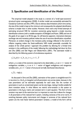
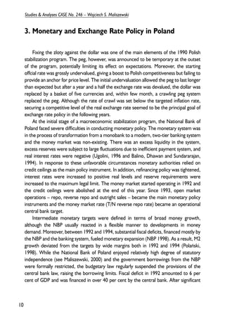
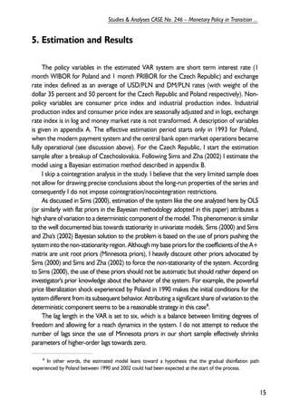
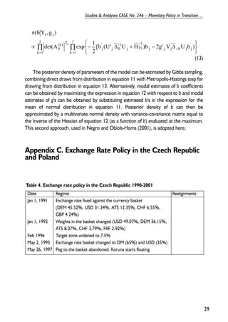
![where Qj is a nk x nk matrix with rank qj and Rj is a mk x mk matrix with rank rj.
Denoting by Uj a nk x qj matrix such that the columns of Uj form an orthonormal basis for
the null space of Qj and denoting by Vj a mk x rj matrix such that the columns of Vj form
an orthonormal space for the null space of Rj, I can express aj and dj in terms of a qj x nk
vector bj and a rj x mk vector gj satisfying the following relationships:
(6)
Vectors bj and gj contain "free" parameters of the model and the original parameters
in aj and dj can be recovered by linear transformations Uj and Vj.
The prior for coefficients in bj and gj are obtained by combining equations 3, 4 and 6:
(7)
(8)
b ~ N(0,H ), j 1,...,n
j 0 j
where
=
H = (U (I ⊗ H )U ) , j =
1,...,n
Introducing notation:
1
’
t
) k (1
x
.
, , k=1,2
(k) and tTk
’
t
) k (1
y
.
.
.
where Tk is the total number of observations in regime k; and t1
(k) are
respectively the first and the last observation from regime k, the likelihood function
expressed in terms of original parameters is proportional to:
27
Studies & Analyses CASE No. 246 – Monetary Policy in Transition ...
a0, j = Ujb j ,d j = Vjg j , j =1,...,n
g ~ N(0,H ), j 1,...,n
j j
=
+
H (V (I H )V ) , j 1,...,n
j
1j
0
’j
j
1
j
1j
0
’
0 j j
− −
+
= ⊗ =
− −
=
’
t
(k)
(k )
Tk
y
Y
=
’
t
(k)
(k )
Tk
x
X
det( exp 1
k T k k k k k k k k k k
Π Π
L A trace Y A X D SA Y A X D SA
k k
= =
det( exp 1
Π Π
A k
Y a X d Sa Y a X d Sa
k k
= =
[ ( )] [ ( )]
2
[ ( )] [ ( )]
2
det( exp 1
Π Π
= =
=
=
− − + + + +
− − + − +
=
∝ − − + − +
2
1
2
1
( )
0,
( ) ( )’ ( ) ( )
0,
( ) ( )
0,
( ) ’ ( )’ ( )
0,
( ) ( )
0,
’( ) ( )’ ( )
0,
) (0
2
1
2
1
( )
0,
( ) ( ) ( )
0,
( ) ’ ( )
0,
( ) ( ) ( )
0,
) ( ) (0
2
1
2
1
) (0
) ( ) ( ) (0
) ( ’ ) (0
) ( ) ( ) (0
) ( ) (0
[ 2( ) ( )’ ( )]
2
k k
k
j
k
j
k k k
j
k
j
k
j
k k k
j
k
j
k
j
k k k
j
k T
k
j
k
j
k k
j
k k
j
k
j
k k
j
k T k
A k
a Y Y a d Sa X Y a d Sa X X d Sa
k](https://image.slidesharecdn.com/sa246-141105085230-conversion-gate02/85/CASE-Network-Studies-and-Analyses-246-Monetary-Policy-in-Transition-Structural-Econometric-Modelling-and-Policy-Simulations-27-320.jpg)
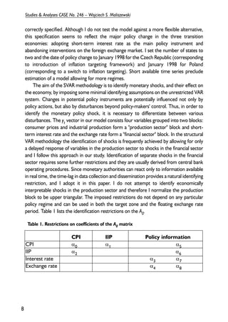
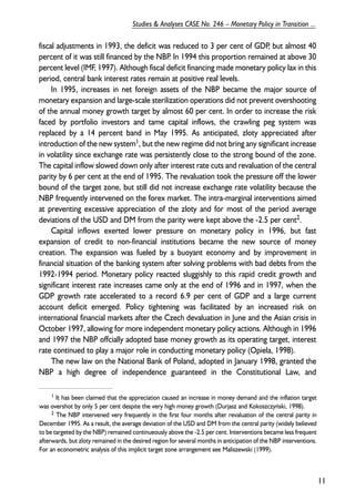
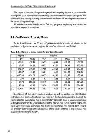
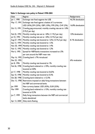
![The above expression can be simplified by introducing the following notation:
~ diag [Y Y 2S’X Y S’X X S]
diag [X(k)’X(k) ] =
where is a matrix X(1)'X(1) and X(2)'X(2) on the diagonal.
Using the newly introduced symbols, the likelihood function is proportional
to:
(9)
2
L det(A k
exp 1 (k) T
0 d ] [a ~ a 2d’ ~ a d ~
Equation 9 can be re-written in terms of free parameters bj and gj implicitly defined
in equation 6:
(10)
2
L det(A k
exp 1 (k) T
0 V g ] [b U’ ~ U b 2g’ V ~ U b g V ~
Combining equation 10 with priors from equation 8 and 7, and completing the
squares in gj gives the following conditional posterior distribution for gj and the marginal
density kernel for b:
(11)
where
(12)
2
det(A exp 1
where
1 ’jj U )]b ~ V ( ) H V ~ V ( g ~
Alternatively, combining equation 10 with priors from equation 7 gives the following
π
conditional density kernel for b:
28
Studies & Analyses CASE No. 246 – Wojciech S. Maliszewski
{ }
{ 2 }
k 1
(k)’ (k) (k)’ (k)
0
2
k 1
1 (k)’ (k) (k)’ (k) (k)’ (k)
0
~ diag [X Y X X S]
+ =
=
−
Δ = −
Δ = − +
{ 2 }
k 1
~ 1 diag [X(k)’X(k) ]
=
−
Δ+ =
{ 2 }
k 1
Π Π
= =
−
+ +
−
∝ − Δ − Δ + Δ
k 1
2
k 1
j
’ 1
0,j j 0 0, j j
1
0
’
0,j
2
Π Π
= =
−
+ +
−
∝ − Δ − Δ + Δ
k 1
2
k 1
j j
1 ’j
’
0 j j j
’j
j j j
1
j 0
’
j
2
) ) H V ~ zV ( , g ~
( ) b , Y g ( 1 1j
j
1 ’j
j T j
− −+
−
π = Ν Δ+ +
Π Π
= =
+
− −+
−
+ +
− −
∝ − Δ + − Δ Δ + Δ
k 1
2
k 1
0 j j
’j
1 1j
j
1 ’j
0 j
’j
j
1j
j 0
1
j 0
’
j
(k) T
0
t j
[b (U’ ~ U H )b (V ~ U )’(V ~ V H ) (V ~ U )]b
2
(bY ,g )
k
0 j j
’j
1 1j
j
+
− −+
−
= Δ+ + Δ](https://image.slidesharecdn.com/sa246-141105085230-conversion-gate02/85/CASE-Network-Studies-and-Analyses-246-Monetary-Policy-in-Transition-Structural-Econometric-Modelling-and-Policy-Simulations-28-320.jpg)

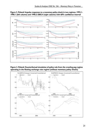
This document discusses monetary policy in Poland between 1990 and 1995. It begins by describing Poland's initial stabilization program which involved fixing the zloty to the dollar. Over time, Poland transitioned to a crawling peg system with the zloty tied to a basket of currencies. Interest rates and credit ceilings were initially used as monetary policy tools, but open market operations became the main instrument from 1993 onward. Fiscal deficits in the early 1990s complicated monetary policy implementation. The document then analyzes various monetary and exchange rate policy changes in Poland during this period.


