Download to read offline
![Studies & Analyses CASE No. 248 – Przemyslaw Kowalski, Wojciech Paczynski, Lukasz Rawdanowicz
2.3. Introducing sectoral differentiation
10
While the aggregate Mundell-Fleming and AS/AD models do not explicitly tackle adjustments
in tradables and nontradables, they do provide predictions about short-term changes in income
levels and real exchange rate changes, as illustrated above. It can be argued that the analysis of
underlying shocks and resulting adjustments in real exchange rates and incomes is only a step
away from analysis of adjustments in tradables and nontradables.
Assuming equal income elasticity of demand in the two sectors4 and imperfect substitutability
between tradables and nontradables, we can make some approximate predictions about the likely
relative exposure of sectors producing tradables and nontradables to different shocks under
floating and fixed exchange rate regimes. If, as a result of a given shock, only income changes,
both sectors should experience proportionate changes in demand. In this case, conclusions related
to the desirability of a given exchange rate regime drawn from aggregate analysis can be extended
to the sectoral dimension. However, if income shifts coincide with exchange rate changes, the two
sectors will be affected differently.
This line of reasoning, coupled with the Calvo (1999a) model described above, confirms this
intuitive result: under a fixed exchange rate regime demand in both sectors will be affected
proportionally [var(y)=var(u); var(e)=0]. The same finding is obtained with the full exchange rate
pass-through. Under a floating exchange rate regime with less than full pass-through, however,
var(y) = var(v) and var(e) = (var(v) + var(u) + 2cov(u,v) / a2), implying that tradables and
nontradables will be affected proportionately only under the condition that var(v) + var(u) = -
2cov(u,v), which is a special case of perfect negative correlation of shocks to IS and LM curves
and cannot be presumed a priori.
These results from the very general variation of the IS/LM model in Calvo (1999a) can be
extended to more traditional versions of this model in which shocks to fiscal policy, foreign income,
foreign price level and interest rates can be analysed explicitly if one identifies real exchange rate
(in)stability with the relative (in)stability of sectors. This idea has been implemented by Dehejia and
Rowe (2001), who considered real exchange rate stability as one of the criteria for an assessment
of monetary regimes.
Dehejia and Rowe (2001) propose a version of the flexible price Mundell-Fleming model with
stochastic components in aggregate demand and supply and compare the variance of aggregate
output and of the expected real exchange rate and the expected interest rate, all relative to their
natural rates under different monetary rules. They consider the variance of the expected real
exchange rate as a proxy for stabilisation of tradables and the variance of the expected real
interest rate as an indicator of stability in the interest rate sensitive sector. Natural rates are defined
as those that would prevail if no price surprises occurred (i.e., when the actual price level meets
4 If a representative consumer makes the choice between tradables and nontradables according to the Cobb-
Douglas type of utility function, shares of expenditure devoted to tradables and nontradables will be constant, and the
unit increase in income, ceteris paribus, will increase demand in both sectors by the same amount.](https://image.slidesharecdn.com/sa248-141105074112-conversion-gate01/75/CASE-Network-Studies-and-Analyses-248-Exchange-Rate-Regimes-and-the-Real-Sector-a-Sectoral-Analysis-of-CEE-Countries-10-2048.jpg)


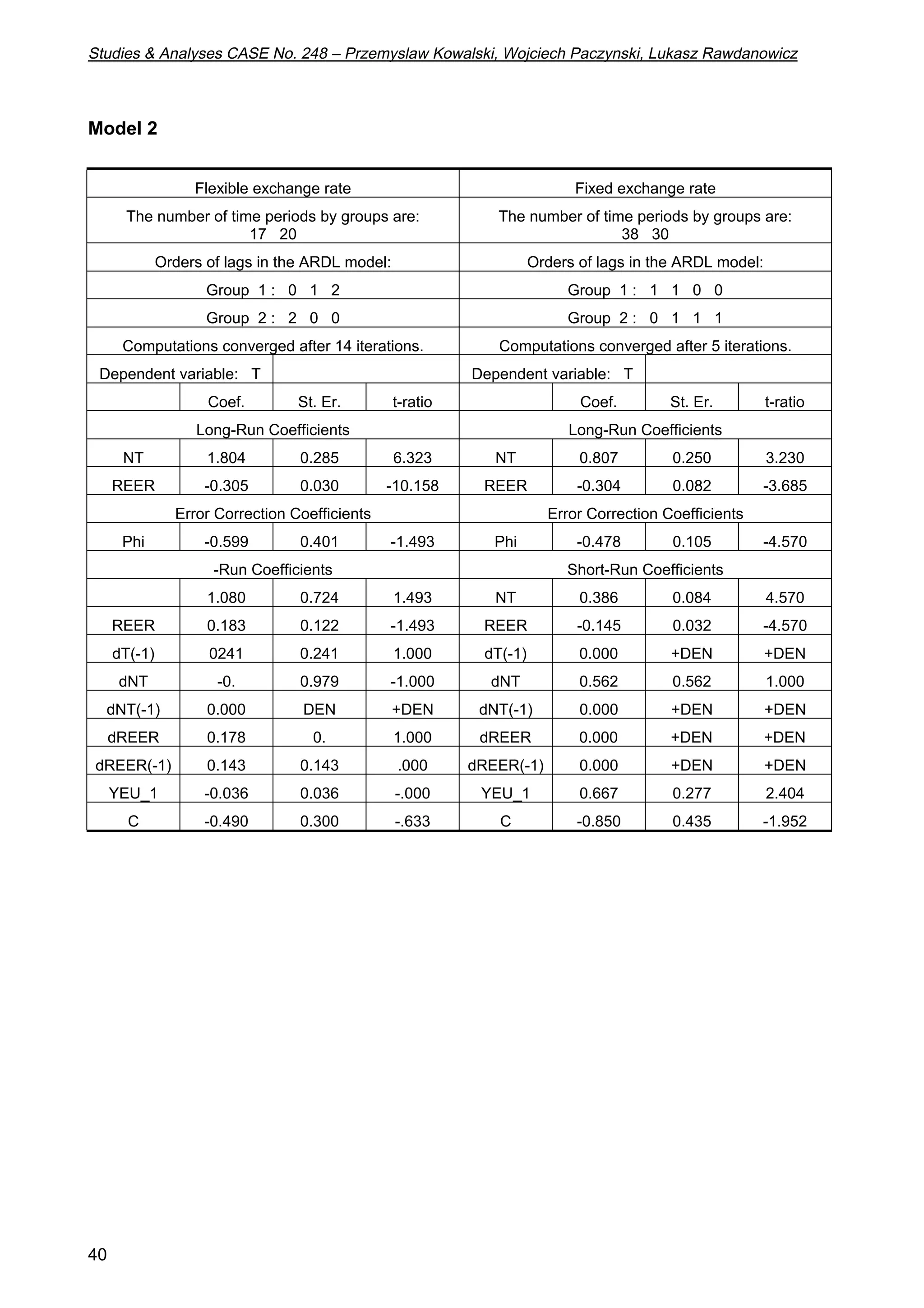
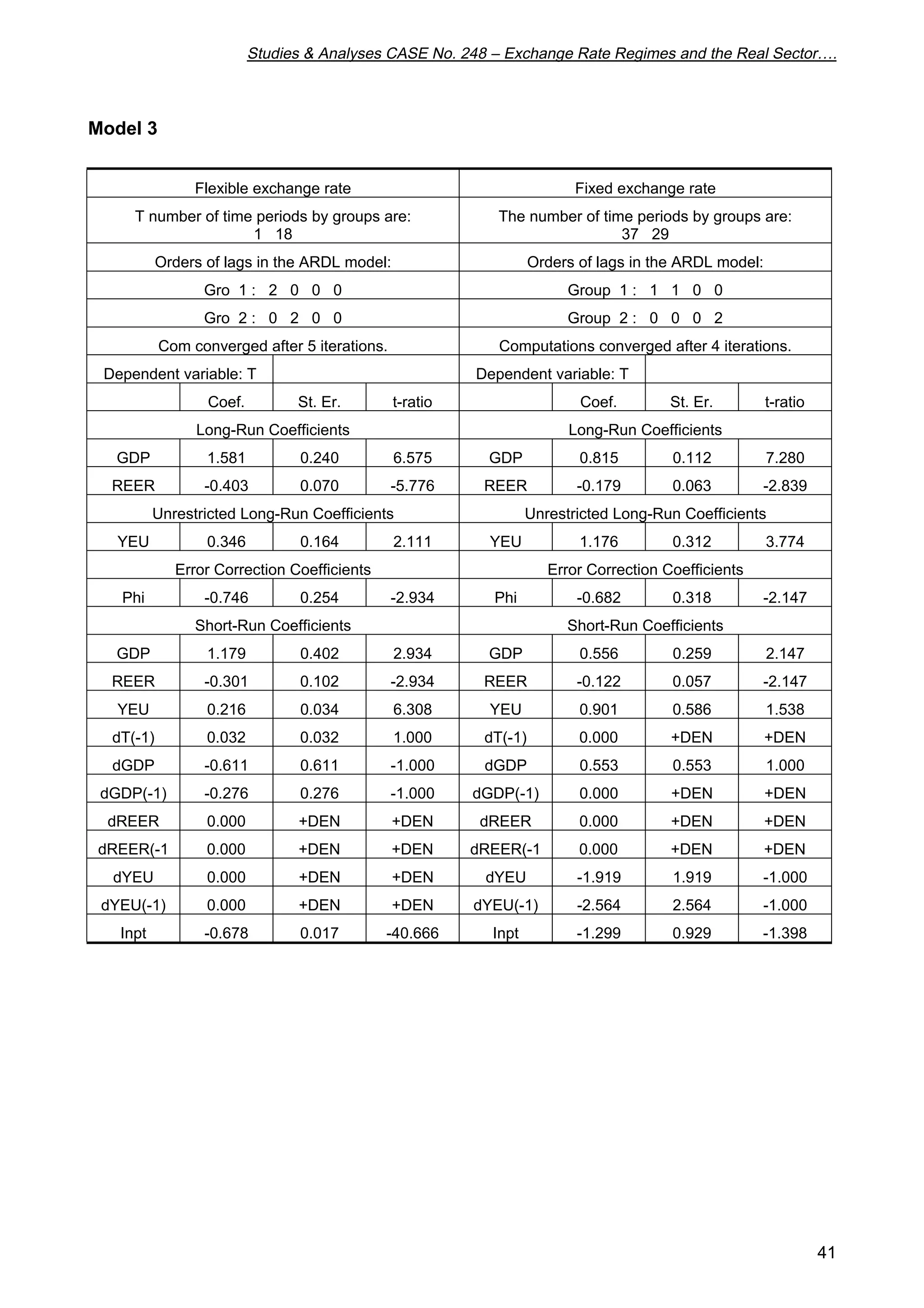
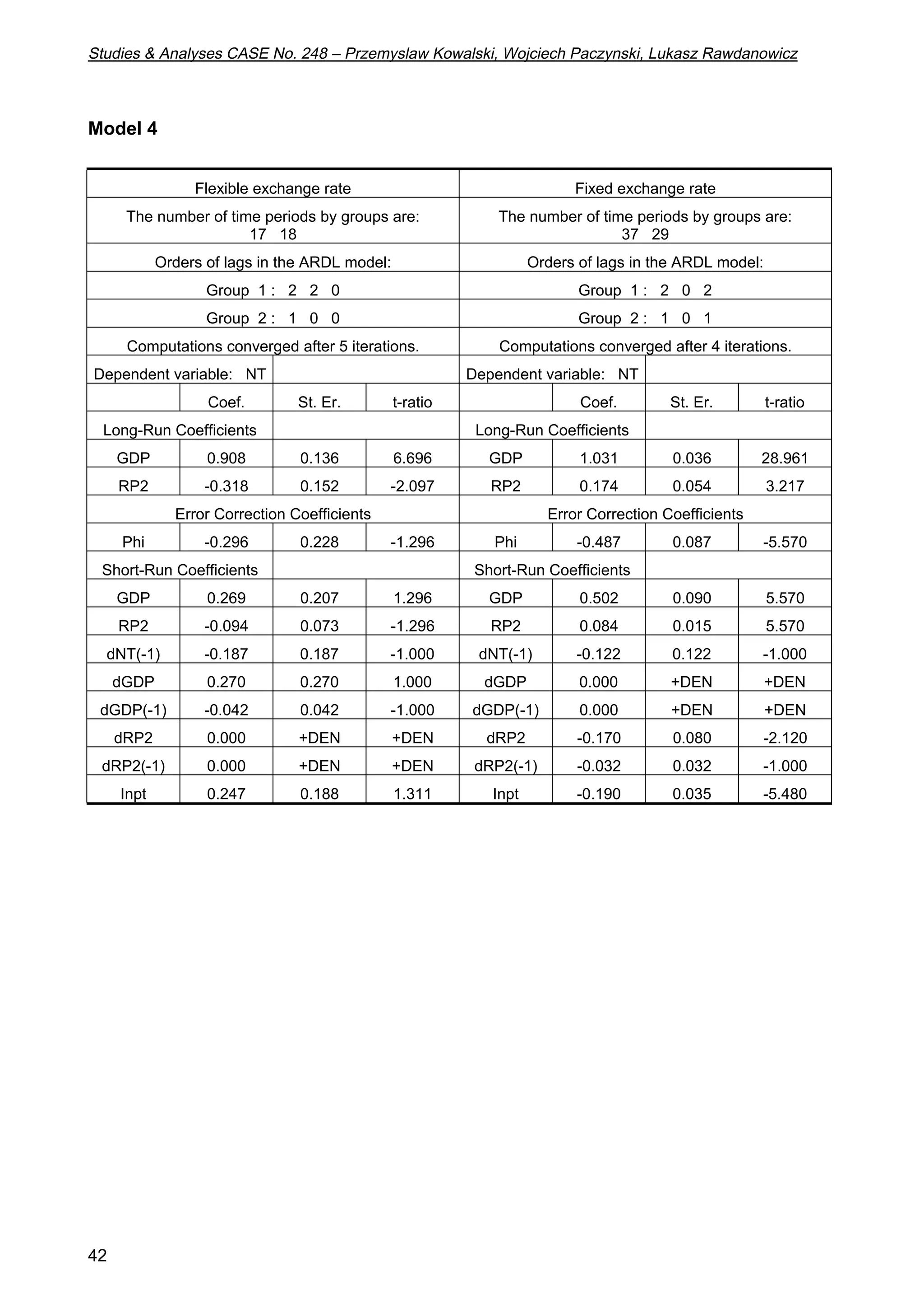

This paper analyzes the impact of exchange rate regimes on the real sectors of seven Central and Eastern European countries by distinguishing between tradable and nontradable sectors. It finds no firm evidence of differential effects of exchange rate regimes on output and prices within these sectors, despite the theoretical expectation of such impacts. The study provides a critical survey of existing literature and empirical evidence, aiming to fill the gap in sector-specific analyses in exchange rate regime discussions.


