RVO-STATISTICS

1. Introduction To Statistics

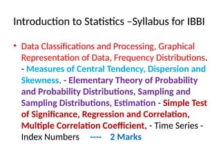
2. Introduction to Statistics –Syllabus for IBBI
• Data Classifications and Processing, Graphical
Representation of Data, Frequency Distributions.
- Measures of Central Tendency, Dispersion and
Skewness. - Elementary Theory of Probability
and Probability Distributions, Sampling and
Sampling Distributions, Estimation - Simple Test
of Significance, Regression and Correlation,
Multiple Correlation Coefficient, - Time Series -
Index Numbers ---- 2 Marks

3. Why study statistics?
1. Data are everywhere
2. Statistical techniques are used to make many
decisions that affect our lives
3. No matter what your career, you will make
professional decisions that involve data. An
understanding of statistical methods will help you
make these decisions efectively
4. Statistics is used in various disciplines such as
psychology, business, physical and social sciences,
humanities, government, and manufacturing.

4. MEANING OF STATISTICS
• The word ‘ Statistics’ and ‘ Statistical’ are all
derived from the Latin word Status, means a
political state.
• The science of collecting, organizing,
presenting, analyzing and interpreting data to
assist in making more effective decisions
• Statistical analysis – used to manipulate
summarize, and investigate data, so that useful
decision-making information results.

5. Applications of statistical concepts in
the business world
• Finance – correlation and regression, index
numbers, time series analysis
• Marketing – Index Numbers, time series analysis ,
nonparametric statistics
• Personel – hypothesis testing, chi-square tests,
nonparametric tests
• Operating management – hypothesis testing,
estimation, analysis of variance, time series analysis

6. Types of statistics
• Descriptive statistics – Methods of organizing,
summarizing, and presenting data in an informative
way
• Inferential statistics – The methods used to
determine something about a population on the
basis of a sample
– Population –The entire set of individuals or objects of
interest or the measurements obtained from all
individuals or objects of interest
– Sample – A portion, or part, of the population of interest

7. FOUR STAGES OF STATISTICS
• 1. Collection of Data: It is the first step and this is the
foundation upon which the entire data set.
• 2. Presentation of data: The mass data collected should be
presented in a suitable, concise form for further analysis.
• 3. Analysis of data: The data presented should be carefully
analysed for making inference from the presented data such
as measures of central tendencies, dispersion, correlation,
regression etc.,
• 4. Interpretation of data: The final step is drawing
conclusion from the data collected. A valid conclusion must
be drawn on the basis of analysis

8. DATA
Statistical data are usually obtained by counting or
measuring items. Most data can be put into the
following categories:
• Qualitative - data are measurements that each fail
into one of several categories. (hair color, ethnic
groups and other attributes of the population)
• quantitative - data are observations that are
measured on a numerical scale (distance traveled to
college, number of children in a family, etc.)

9. Frequency distributions – numerical
presentation of quantitative data
• Frequency distribution – shows the frequency,
or number of occurences, in each of several
categories. Frequency distributions are used to
summarize large volumes of data values.
• When the raw data are measured on a
qunatitative scale, either interval or ration,
categories or classes must be designed for the
data values before a frequency distribution can
be formulated.

10. Charts and graphs
• Frequency distributions are good ways to present the essential aspects of data
collections in concise and understable terms
• Pictures are always more effective in displaying large data collections
• One-dimensional diagrams (Line, Simple, Multiple Bar diagram, Sub-divided bar
diagram)
• Two-dimensional diagrams (Rectangle, Circles and Squares)
• Three-dimensional diagrams (cubes, cylinders,spheres, etc.)
• Pictograms and Cartograms
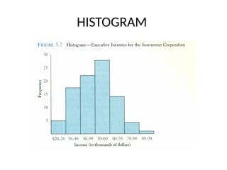
• Histogram:
• Frequently used to graphically present interval and ratio data.
• Is often used for interval and ratio data.
• The adjacent bars indicate that a numerical range is being summarized by
indicating the frequencies in arbitrarily chosen classes

11. HISTOGRAM

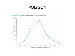
12. Frequency polygon
• Another common method for graphically
presenting interval and ratio data
• To construct a frequency polygon mark the
frequencies on the vertical axis and the values
of the variable being measured on the
horizontal axis, as with the histogram.
• If the purpose of presenting is comparation
with other distributions, the frequency polygon
provides a good summary of the data

13. POLYGON

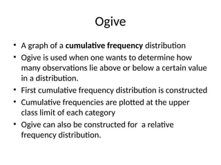
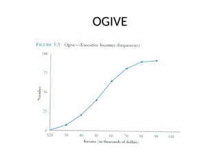
14. Ogive
• A graph of a cumulative frequency distribution
• Ogive is used when one wants to determine how
many observations lie above or below a certain value
in a distribution.
• First cumulative frequency distribution is constructed
• Cumulative frequencies are plotted at the upper
class limit of each category
• Ogive can also be constructed for a relative
frequency distribution.

15. OGIVE

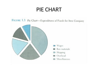
16. Pie Chart
• The pie chart is an effective way of displaying
the percentage breakdown of data by
category.
• Useful if the relative sizes of the data
components are to be emphasized
• Pie charts also provide an effective way of
presenting ratio- or interval-scaled data after
they have been organized into categories

17. PIE CHART

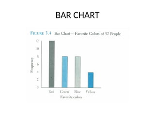
18. Bar chart
• Another common method for graphically presenting
nominal and ordinal scaled data
• One bar is used to represent the frequency for each
category
• The bars are usually positioned vertically with their
bases located on the horizontal axis of the graph
• The bars are separated, and this is why such a graph is
frequently used for nominal and ordinal data – the
separation emphasize the plotting of frequencies for
distinct categories

19. BAR CHART

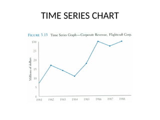
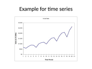
20. Time Series Graph
• The time series graph is a graph of data that
have been measured over time.
• The horizontal axis of this graph represents
time periods and the vertical axis shows the
numerical values corresponding to these time
periods

21. TIME SERIES CHART

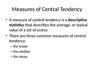
22. Measures of Central Tendency
• A measure of central tendency is a descriptive
statistics that describes the average, or typical
value of a set of scores
• There are three common measures of central
tendency:
– the mode
– the median
– the mean

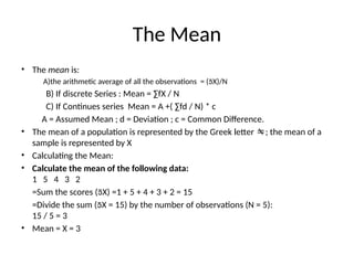
23. The Mean
• The mean is:
A)the arithmetic average of all the observations = (X)/N
B) If discrete Series : Mean = ∑fX / N
C) If Continues series Mean = A +( ∑fd / N) * c
A = Assumed Mean ; d = Deviation ; c = Common Difference.
• The mean of a population is represented by the Greek letter ; the mean of a
sample is represented by X
• Calculating the Mean:
• Calculate the mean of the following data:
1 5 4 3 2
=Sum the scores (X) =1 + 5 + 4 + 3 + 2 = 15
=Divide the sum (X = 15) by the number of observations (N = 5):
15 / 5 = 3
• Mean = X = 3

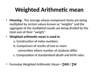
24. Weighted Arithmetic mean
• Meaning : The average whose component items are being
multiplied by certain values known as “weights” and the
aggregate of the multiplied results are being divided by the
total sum of their “weight”.
• Weighted arithmetic mean is used in:
a. Construction of index numbers.
b. Comparison of results of two or more
universities where number of students differ.
c. Computation of standardized death and birth rates.
• Formulae Weighted Arithmetic Mean = ∑WX / ∑W

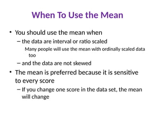
25. When To Use the Mean
• You should use the mean when
– the data are interval or ratio scaled
Many people will use the mean with ordinally scaled data
too
– and the data are not skewed
• The mean is preferred because it is sensitive
to every score
– If you change one score in the data set, the mean
will change

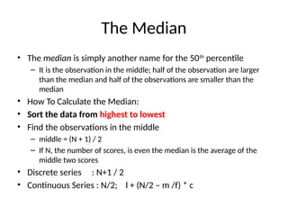
26. The Median
• The median is simply another name for the 50th
percentile
– It is the observation in the middle; half of the observation are larger
than the median and half of the observations are smaller than the
median
• How To Calculate the Median:
• Sort the data from highest to lowest
• Find the observations in the middle
– middle = (N + 1) / 2
– If N, the number of scores, is even the median is the average of the
middle two scores
• Discrete series : N+1 / 2
• Continuous Series : N/2; l + (N/2 – m /f) * c

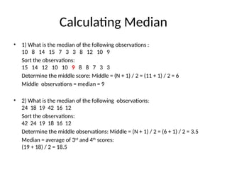
27. Calculating Median
• 1) What is the median of the following observations :
10 8 14 15 7 3 3 8 12 10 9
Sort the observations:
15 14 12 10 10 9 8 8 7 3 3
Determine the middle score: Middle = (N + 1) / 2 = (11 + 1) / 2 = 6
Middle observations = median = 9
• 2) What is the median of the following observations:
24 18 19 42 16 12
Sort the observations:
42 24 19 18 16 12
Determine the middle observations: Middle = (N + 1) / 2 = (6 + 1) / 2 = 3.5
Median = average of 3rd
and 4th
scores:
(19 + 18) / 2 = 18.5

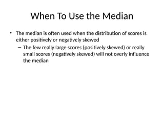
28. When To Use the Median
• The median is often used when the distribution of scores is
either positively or negatively skewed
– The few really large scores (positively skewed) or really
small scores (negatively skewed) will not overly influence
the median

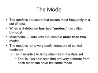
29. The Mode
• The mode is the score that occurs most frequently in a
set of data
• When a distribution has two “modes,” it is called
bimodal
• Multimodal -- Data sets that contain more than two
modes
• The mode is not a very useful measure of central
tendency
– It is insensitive to large changes in the data set
• That is, two data sets that are very different from
each other can have the same mode

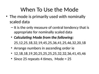
30. When To Use the Mode
• The mode is primarily used with nominally
scaled data
– It is the only measure of central tendency that is
appropriate for nominally scaled data
• Calculating Mode from the following:
25,12,25,18,32,19,45,25,36,41,25,46,32,20,18
• Arrange numbers in ascending order ie
• 12,18,18,19,20,25,25,25,25,32,32,36,41,45,46
• Since 25 repeats 4 times, Mode = 25

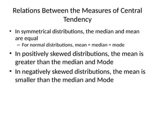
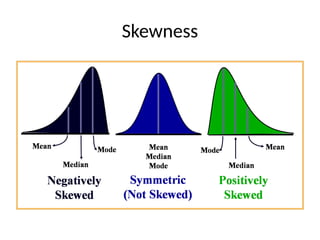
31. Relations Between the Measures of Central
Tendency
• In symmetrical distributions, the median and mean
are equal
– For normal distributions, mean = median = mode
• In positively skewed distributions, the mean is
greater than the median and Mode
• In negatively skewed distributions, the mean is
smaller than the median and Mode

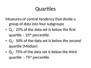
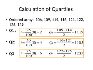
32. Quartiles
Measures of central tendency that divide a
group of data into four subgroups
• Q1: 25% of the data set is below the first
quartile – 25th
percentile
• Q2: 50% of the data set is below the second
quartile (Median)
• Q3: 75% of the data set is below the third
quartile - 75th
percentile

33. Calculation of Quartiles
• Ordered array: 106, 109, 114, 116, 121, 122,
125, 129
• Q1 :
• Q2:
• Q3

34. Meaning and Features of Dispersion
The measure of central tendency serve to locate the center of
the distribution, but they do not reveal how the items are out on
either side of center.
In a series all the items are not equal. There is difference or
variation among the values. The degree of variation is
evaluated by various measures of dispersion.
Use of dispersion measures:
a) To determine the reliability of an average.
b) To compare two or more series with regard to their
variability.
c) To facilitate the use of other statistical measures.

35. Kinds of measures of dispersion
• There are two kinds of measures of dispersion:
• 1. Absolute measure of dispersion: The amount of
variation in a set of values in terms of observation.
Examples: Range, Quartile deviation, Mean deviation and
Standard deviation
• 2. Relative measure of dispersion: They are used to
compare the variations in two or more sets, which are
having different units of measurement of observations.
Example: Coefficient of range, Coefficient of quartile
deviation, coefficient of Mean deviation and Coefficient of
variation.

36. Measures of Variability
• Measures of variability describe the spread or the
dispersion of a set of data.
• Common Measures of Variability
–Range
–Interquartile Range
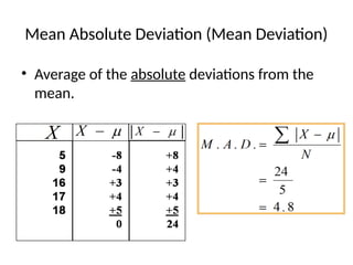
–Mean Absolute Deviation
–Variance
–Standard Deviation
–Coefficient of Variation

37. RANGE
• The difference between the largest and the
smallest values in a set of data
• Simple to compute
• Ignores all data points except the two
extremes
• Example:
• Range =Largest – Smallest = 48 - 35 = 13

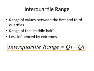
38. Interquartile Range
• Range of values between the first and third
quartiles
• Range of the “middle half”
• Less influenced by extremes

39. Mean Absolute Deviation (Mean Deviation)
• Average of the absolute deviations from the
mean.

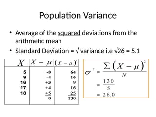
40. Population Variance
• Average of the squared deviations from the
arithmetic mean
• Standard Deviation = √ variance i.e √26 = 5.1

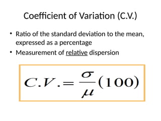
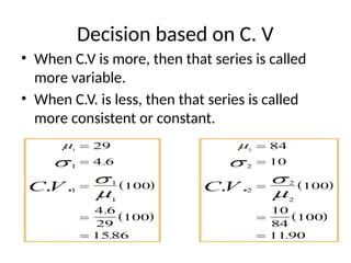
41. Coefficient of Variation (C.V.)
• Ratio of the standard deviation to the mean,
expressed as a percentage
• Measurement of relative dispersion

42. Decision based on C. V
• When C.V is more, then that series is called
more variable.
• When C.V. is less, then that series is called
more consistent or constant.

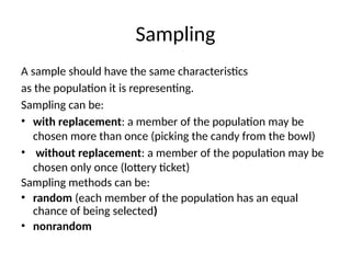
43. Sampling
A sample should have the same characteristics
as the population it is representing.
Sampling can be:
• with replacement: a member of the population may be
chosen more than once (picking the candy from the bowl)
• without replacement: a member of the population may be
chosen only once (lottery ticket)
Sampling methods can be:
• random (each member of the population has an equal
chance of being selected)
• nonrandom

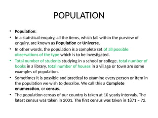
44. POPULATION
• Population:
• In a statistical enquiry, all the items, which fall within the purview of
enquiry, are known as Population or Universe.
• In other words, the population is a complete set of all possible
observations of the type which is to be investigated.
• Total number of students studying in a school or college, total number of
books in a library, total number of houses in a village or town are some
examples of population.
• Sometimes it is possible and practical to examine every person or item in
the population we wish to describe. We call this a Complete
enumeration, or census.
• The population census of our country is taken at 10 yearly intervals. The
latest census was taken in 2001. The first census was taken in 1871 – 72.

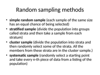
45. Random sampling methods
• simple random sample (each sample of the same size
has an equal chance of being selected)
• stratified sample (divide the population into groups
called strata and then take a sample from each
stratum)
• cluster sample (divide the population into strata and
then randomly select some of the strata. All the
members from these strata are in the cluster sample.)
• systematic sample (randomly select a starting point
and take every n-th piece of data from a listing of the
population)

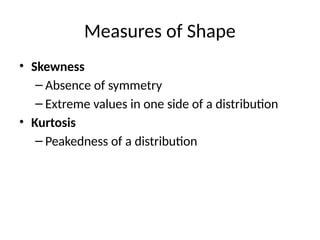
46. Measures of Shape
• Skewness
– Absence of symmetry
– Extreme values in one side of a distribution
• Kurtosis
– Peakedness of a distribution

47. Skewness

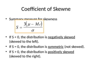
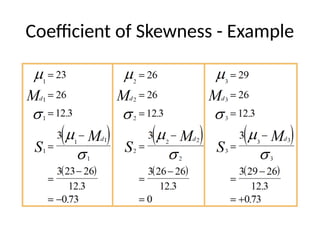
48. Coefficient of Skewne
• Summary measure for skewness
• If S < 0, the distribution is negatively skewed
(skewed to the left).
• If S = 0, the distribution is symmetric (not skewed).
• If S > 0, the distribution is positively skewed
(skewed to the right).

49. Coefficient of Skewness - Example

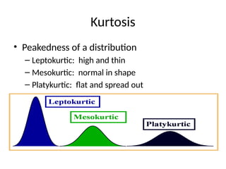
50. Kurtosis
• Peakedness of a distribution
– Leptokurtic: high and thin
– Mesokurtic: normal in shape
– Platykurtic: flat and spread out

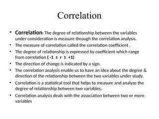
51. Correlation
• Correlation: The degree of relationship between the variables
under consideration is measure through the correlation analysis.
• The measure of correlation called the correlation coefficient .
• The degree of relationship is expressed by coefficient which range
from correlation ( -1 ≤ r ≥ +1)
• The direction of change is indicated by a sign.
• The correlation analysis enable us to have an idea about the degree &
direction of the relationship between the two variables under study.
• Correlation is a statistical tool that helps to measure and analyze the
degree of relationship between two variables.
• Correlation analysis deals with the association between two or more
variables

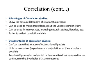
52. Correlation (cont...)
• Advantages of Correlation studies:
• Show the amount (strength) of relationship present
• Can be used to make predictions about the variables under study.
• Can be used in many places, including natural settings, libraries, etc.
• Easier to collect co relational data
• Disadvantages of correlation studies:
• Can’t assume that a cause-effect relationship exists
• Little or no control (experimental manipulation) of the variables is
possible
• Relationships may be accidental or due to a third, unmeasured factor
common to the 2 variables that are measured

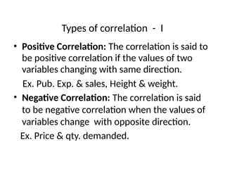
53. Types of correlation - I
• Positive Correlation: The correlation is said to
be positive correlation if the values of two
variables changing with same direction.
Ex. Pub. Exp. & sales, Height & weight.
• Negative Correlation: The correlation is said
to be negative correlation when the values of
variables change with opposite direction.
Ex. Price & qty. demanded.

54. Types of Correlation Type II
• Simple correlation: Under simple correlation
problem there are only two variables are studied.
• Multiple Correlation: Under Multiple Correlation
three or more than three variables are studied.
Ex. Qd = f ( P,PC, PS, t, y )
• Partial correlation: analysis recognizes more than
two variables but considers only two variables
keeping the other constant.
• Total correlation: is based on all the relevant
variables, which is normally not feasible.

55. Methods of Studying Correlation
• Scatter Diagram Method
• Graphic Method
• Karl Pearson’s Coefficient of Correlation
• Method of Least Square

56. Scatter Diagram Method
• Scatter Diagram is a graph of observed plotted points where
each points represents the values of X & Y as a coordinate. It
portrays the relationship between these two variables
graphic
• Advantages of Scatter Diagram
• Simple & Non Mathematical method
• Not influenced by the size of extreme item
• First step in investing the relationship between two variables
• Disadvantage of scatter diagram : Can not adopt the an exact
degree of correlation

57. Karl Pearson's
Coefficient of Correlation
• Karl Pearson’s Coefficient of Correlation denoted by-
‘r’ The coefficient of correlation ‘r’ measure the
degree of linear relationship between two variables
say x & y
 Karl Pearson’s Coefficient of Correlation denoted
by- r = -1 ≤ r ≥ +1
 Degree of Correlation is expressed by a value of
Coefficient
 Direction of change is Indicated by sign ( - ve) or ( +
ve)

58. Interpretation of Correlation Coefficient
(r)
• The value of correlation coefficient ‘r’ ranges
from -1 to +1
• If r = +1, then the correlation between the two
variables is said to be perfect and positive
• If r = -1, then the correlation between the two
variables is said to be perfect and negative
• If r = 0, then there exists no correlation
between the variables

59. Karl Pearson's
Coefficient of Correlation (Cont..)
• Advantages of Pearson’s Coefficient : It summarizes
in one value, the degree of correlation & direction of
correlation also.
• Limitation of Pearson’s Coefficient :
• Always assume linear relationship
• Interpreting the value of r is difficult.
• Value of Correlation Coefficient is affected by the
extreme values.
• Time consuming methods

60. Interpretation of Rank Correlation
Coefficient (R)
• The value of rank correlation coefficient, R
ranges from -1 to +1
• If R = +1, then there is complete agreement in
the order of the ranks and the ranks are in the
same direction
• If R = -1, then there is complete agreement in
the order of the ranks and the ranks are in the
opposite direction
• If R = 0, then there is no correlation

61. Regression Analysis
• Regression Analysis is a very powerful tool in the
field of statistical analysis in predicting the value of
one variable, given the value of another variable,
when those variables are related to each other.
• Regression Analysis is mathematical measure of
average relationship between two or more
variables.
• Regression analysis is a statistical tool used in
prediction of value of unknown variable from
known variable.

62. Regression Analysis (cont..)
• Advantages of Regression Analysis:
• Regression analysis provides estimates of values of the dependent
variables from the values of independent variables.
• Regression analysis also helps to obtain a measure of the error involved
in using the regression line as a basis for estimations .
• Regression analysis helps in obtaining a measure of the degree of
association or correlation that exists between the two variable.
• Disadvantages of Regression Analysis:
• To the extent forecasts of the values of explanatory variables are
incorrect, the forecasts based on regression method will be wrong.
• To the extent the structural changes have taken place,. the past
relationship between independent and dependent variables will not
continue in the future.
• The forecasts under this method assume that the forecast equation
holds exactly in the prediction period. To the' extent it is stochastic, i.e.,
the disturbance term is non-zero, the forecasts will be wrong.

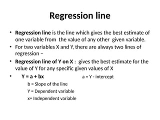
63. Regression line
• Regression line is the line which gives the best estimate of
one variable from the value of any other given variable.
• For two variables X and Y, there are always two lines of
regression –
• Regression line of Y on X : gives the best estimate for the
value of Y for any specific given values of X
• Y = a + bx a = Y - intercept
b = Slope of the line
Y = Dependent variable
x= Independent variable

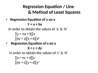
64. Regression Equation / Line
& Method of Least Squares
• Regression Equation of y on x
Y = a + bx
In order to obtain the values of ‘a’ & ‘b’
∑y = na + b∑x
∑xy = a∑x + b∑x2
• Regression Equation of x on y
X = c + dy
In order to obtain the values of ‘c’ & ‘d’
∑x = nc + d∑y
∑xy = c∑y + d∑y2

65. Correlation analysis vs.
Regression analysis.
• Regression is the average relationship between two
variables
• Correlation need not imply cause & effect relationship
between the variables understudy.- R A clearly indicate
the cause and effect relation ship between the variables.
• There may be non-sense correlation between two
variables.- There is no such thing like non-sense
regression.
• Regression is the average relationship between two
variables

66. Time series analysis
• Objectives of time series analysis:

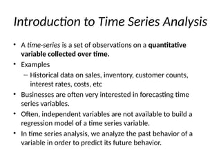
67. Introduction to Time Series Analysis
• A time-series is a set of observations on a quantitative
variable collected over time.
• Examples
– Historical data on sales, inventory, customer counts,
interest rates, costs, etc
• Businesses are often very interested in forecasting time
series variables.
• Often, independent variables are not available to build a
regression model of a time series variable.
• In time series analysis, we analyze the past behavior of a
variable in order to predict its future behavior.

68. Time Series Analysis (TSA)
• A statistical technique that uses time-series data
for explaining the past or forecasting future
events.
• The prediction is a function of time (days,
months, years, etc.)
• No causal variable; examine past behavior of
a variable and and attempt to predict future
behavior

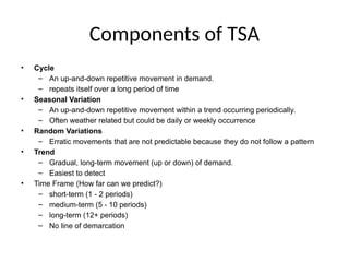
69. Components of TSA
• Cycle
– An up-and-down repetitive movement in demand.
– repeats itself over a long period of time
• Seasonal Variation
– An up-and-down repetitive movement within a trend occurring periodically.
– Often weather related but could be daily or weekly occurrence
• Random Variations
– Erratic movements that are not predictable because they do not follow a pattern
• Trend
– Gradual, long-term movement (up or down) of demand.
– Easiest to detect
• Time Frame (How far can we predict?)
– short-term (1 - 2 periods)
– medium-term (5 - 10 periods)
– long-term (12+ periods)
– No line of demarcation

70. Example for time series

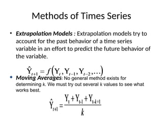
71. Methods of Times Series
• Extrapolation Models : Extrapolation models try to
account for the past behavior of a time series
variable in an effort to predict the future behavior of
the variable.
 Moving Averages: No general method exists for
determining k. We must try out several k values to see what
works best.

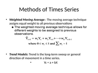
72. Methods of Times Series
• Weighted Moving Average : The moving average technique
assigns equal weight to all previous observations
• Trend Models: Trend is the long-term sweep or general
direction of movement in a time series.
• Yc = a + bX

73. Index Numbers
• An index number is a statistical value that measures the
change in a variable with respect to time
• Two variables that are often considered in this analysis are
price and quantity
• With the aid of index numbers, the average price of several
articles in one year may be compared with the average
price of the same quantity of the same articles in a
number of different years
• There are several sources of ‘official’ statistics that contain
index numbers for quantities such as food prices, clothing
prices, housing, wages and so on

74. CHARACTERISTICS OF INDEX NUMBER
• Following are some of the important characteristics of index numbers : ·
• 1) Index numbers are expressed in terms of percentages to show the
extent of relative change
• 2) Index numbers measure relative changes. They measure the relative
change in the value of a variable or a group of related variables over a
period of time or between places.
• 3)Index numbers measures changes which are not directly measurable.
The cost of living, the price level or the business activity in a country are
not directly measurable but it is possible to study relative changes in
these activities by measuring the changes in the values of
variables/factors which effect these activities.

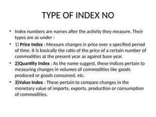
75. TYPE OF INDEX NO
• Index numbers are names after the activity they measure. Their
types are as under :
• 1) Price Index : Measure changes in price over a specified period
of time. It is basically the ratio of the price of a certain number of
commodities at the present year as against base year.
• 2)Quantity Index : As the name suggest, these indices pertain to
measuring changes in volumes of commodities like goods
produced or goods consumed, etc.
• 3)Value Index : These pertain to compare changes in the
monetary value of imports, exports, production or consumption
of commodities.

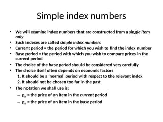
76. Simple index numbers
• We will examine index numbers that are constructed from a single item
only
• Such indexes are called simple index numbers
• Current period = the period for which you wish to find the index number
• Base period = the period with which you wish to compare prices in the
current period
• The choice of the base period should be considered very carefully
• The choice itself often depends on economic factors
1. It should be a ‘normal’ period with respect to the relevant index
2. It should not be chosen too far in the past
• The notation we shall use is:
– pn = the price of an item in the current period
– po = the price of an item in the base period

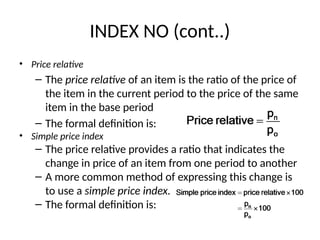
77. INDEX NO (cont..)
• Price relative
– The price relative of an item is the ratio of the price of
the item in the current period to the price of the same
item in the base period
– The formal definition is:
• Simple price index
– The price relative provides a ratio that indicates the
change in price of an item from one period to another
– A more common method of expressing this change is
to use a simple price index.
– The formal definition is:

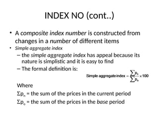
78. INDEX NO (cont..)
• A composite index number is constructed from
changes in a number of different items
• Simple aggregate index
– the simple aggregate index has appeal because its
nature is simplistic and it is easy to find
– The formal definition is:
Where
Spn = the sum of the prices in the current period
Spo = the sum of the prices in the base period

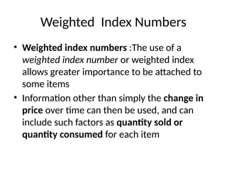
79. Weighted Index Numbers
• Weighted index numbers :The use of a
weighted index number or weighted index
allows greater importance to be attached to
some items
• Information other than simply the change in
price over time can then be used, and can
include such factors as quantity sold or
quantity consumed for each item

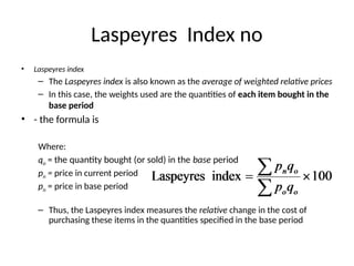
80. Laspeyres Index no
• Laspeyres index
– The Laspeyres index is also known as the average of weighted relative prices
– In this case, the weights used are the quantities of each item bought in the
base period
• - the formula is
Where:
qo = the quantity bought (or sold) in the base period
pn = price in current period
po = price in base period
– Thus, the Laspeyres index measures the relative change in the cost of
purchasing these items in the quantities specified in the base period

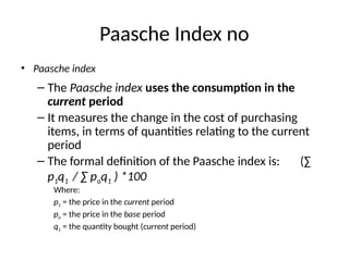
81. Paasche Index no
• Paasche index
– The Paasche index uses the consumption in the
current period
– It measures the change in the cost of purchasing
items, in terms of quantities relating to the current
period
– The formal definition of the Paasche index is: (∑
p1q1 / ∑ poq1 ) *100
Where:
p1 = the price in the current period
po = the price in the base period
q1 = the quantity bought (current period)

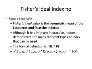
82. Fisher’s Ideal Index no
• Fisher’s ideal index
– Fisher’s ideal index is the geometric mean of the
Laspeyres and Paasche indexes
– Although it has little use in practice, it does
demonstrate the many different types of index
that can be used
– The formal definition is: √(L * P)
– √(∑ p1qo / ∑ poqo ) * (∑ p1q1 / ∑ poq1 ) * 100

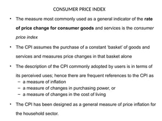
83. CONSUMER PRICE INDEX
• The measure most commonly used as a general indicator of the rate
of price change for consumer goods and services is the consumer
price index
• The CPI assumes the purchase of a constant ‘basket’ of goods and
services and measures price changes in that basket alone
• The description of the CPI commonly adopted by users is in terms of
its perceived uses; hence there are frequent references to the CPI as
– a measure of inflation
– a measure of changes in purchasing power, or
– a measure of changes in the cost of living
• The CPI has been designed as a general measure of price inflation for
the household sector.

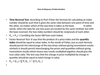
84. Tests of Adequacy of Index Numbers
• Time Reversal Test: According to Prof. Fisher the formula for calculating an index
number should be such that it gives the same ratio between one point of time and
the other, no matter which of the two time is taken as the base. In other
words, when the data for any two years are treated by the same method, but with
the base reversed, the two index numbers should be reciprocals of each other.
• P01 × P10= 1 (omitting the factor l00 from each index).
• Factor Reversal Test: It says that the product of a price index and the quantity
index should be equal to value index. In the words of Fisher, just as each formula
should permit the interchange of the two times without giving inconsistent results
similarly it should permit interchanging the prices and quantities without giving
inconsistent results which means two results multiplied together should give the
true value ratio. The test says that the change in price multiplied by change in
quantity should be equal to total change in value.
• P01 × Q 10= (∑ P1 Q1 ) / (∑ P0 Q 0 )
•

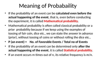
85. Meaning of Probabaility
• If the probability of an event can be calculated even before the
actual happening of the event, that is, even before conducting
the experiment, it is called Mathematical probability.
• Mathematical probability is often called classical probability or a
prior probability because if we keep using the examples of
tossing of fair coin, dice etc., we can state the answer in advance
(prior), without tossing of coins or without rolling the dice etc.,
• P (an event) = No. of Favorable Events / Total no of Events
• If the probability of an event can be determined only after the
actual happening of the event, it is called Statistical probability.
• If an event occurs m times out of n, its relative frequency is m/n.

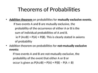
86. Theorems of Probabilities
• Addition theorem on probabilities for mutually exclusive events.
If two events A and B are mutually exclusive, the
probability of the occurrence of either A or B is the
sum of individual probabilities of A and B.
ie P (A B) = P(A) + P(B). This is clearly stated in axioms
∪
of probability
• Addition theorem on probabilities for not-mutually exclusive
events:
If two events A and B are not-mutually exclusive, the
probability of the event that either A or B or
occur is given as P(A B) = P(A) + P(B) – P(A ∩ B)
∪

87. MULTIPLICATION THEOREM
• Multiplication theorem on probabilities for
independent events: If two events A and B are
independent, the probability that both of them occur
is equal to the product of their individual probabilities.
• i.e P(A∩B) = P(A) . P(B)
• Multiplication theorem for dependent events: If A
and B be two dependent events, i.e the occurrence
of one event is affected by the occurrence of the
other event, then the probability that both A and B
will occur is
• ie P(A ∩ B) = P(A) P(B/A)

88. Important discrete probability distribution:
• The binomial Distribution:
•The experiment consists of a sequence of n identical trials
•All possible outcomes can be classified into two categories, usually
called success and failure
•The probability of an success, p, is constant from trial to trial
•The outcome of any trial is independent of the outcome of any
other trial
•Example: The number of heads when tossing a coin for 50 times
• Mean = np,
• variance = npq
• Standard deviation σ = npq

89. POISSON DISTRIBUTION:
Poisson experiments satisfy the following
• The probability of occurrence of an event is the same for any two
intervals of equal length
• The occurrence or non-occurrence of the event in any interval is
independent of the occurrence or non-occurrence in any other
interval
• The probability that two or more events will occur in an interval
approaches zero as the interval becomes smaller In many practical
situations we are interested in measuring how many times a certain
event occurs in a specific time interval or in a specific length or area.
• For instance:
1. The number of phone calls received at an exchange or call centre in
an hour;
2. The number of customers arriving at a toll booth per day;
3. The number of car

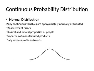
90. Continuous Probability Distribution
• Normal Distribution
Many continuous variables are approximately normally distributed
•Measurement errors
•Physical and mental properties of people
•Properties of manufactured products
•Daily revenues of investments

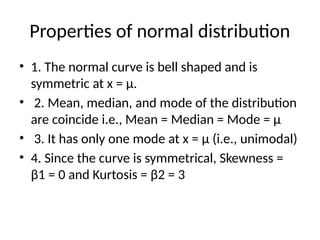
91. Properties of normal distribution
• 1. The normal curve is bell shaped and is
symmetric at x = μ.
• 2. Mean, median, and mode of the distribution
are coincide i.e., Mean = Median = Mode = μ
• 3. It has only one mode at x = μ (i.e., unimodal)
• 4. Since the curve is symmetrical, Skewness =
β1 = 0 and Kurtosis = β2 = 3

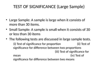
92. TEST OF SIGNIFICANCE (Large Sample)
• Large Sample: A sample is large when it consists of
more than 30 items.
• Small Sample: A sample is small when it consists of 30
or less than 30 items
• The following tests are discussed in large sample tests.
(i) Test of significance for proportion (ii) Test of
significance for difference between two proportions
(iii) Test of significance for
mean (iv) Test of
significance for difference between two means

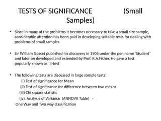
93. TESTS OF SIGNIFICANCE (Small
Samples)
• Since in many of the problems it becomes necessary to take a small size sample,
considerable attention has been paid in developing suitable tests for dealing with
problems of small samples
• Sir William Gosset published his discovery in 1905 under the pen name ‘Student’
and later on developed and extended by Prof. R.A.Fisher. He gave a test
popularly known as ‘ t-test’
• The following tests are discussed in large sample tests:
(i) Test of significance for Mean
(ii) Test of significance for difference between two means
(iii) Chi square statistic
(iv) Analysis of Variance (ANNOVA Table) -
One Way and Two way classification