Basics of Statistics
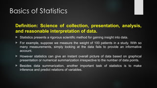
Definition:Science of collection, presentation, analysis,
and reasonable interpretation of data.
Statistics presents a rigorous scientific method for gaining insight into data.
For example, suppose we measure the weight of 100 patients in a study. With so
many measurements, simply looking at the data fails to provide an informative
account.
However statistics can give an instant overall picture of data based on graphical
presentation or numerical summarization irrespective to the number of data points.
Besides data summarization, another important task of statistics is to make
inference and predict relations of variables.
3.
What is Data?
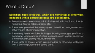
Definition:Facts or figures, which are numerical or otherwise,
collected with a definite purpose are called data.
Everyday we come across a lot of information in the form of facts,
numerical figures, tables, graphs, etc.
These are provided by newspapers, televisions, magazines and
other means of communication.
These may relate to cricket batting or bowling averages, profits of a
company, temperatures of cities, expenditures in various sectors of
a five year plan, polling results, and so on.
These facts or figures, which are numerical or otherwise, collected
with a definite purpose are called data.
5.
Primary Data VsSecondary Data
Primary Data
Primary data is the data that is collected for the first time
through personal experiences or evidence, particularly for
research.
It is also described as raw data or first-hand information.
The mode of assembling the information is costly.
The data is mostly collected through observations, physical
testing, mailed questionnaires, surveys, personal interviews,
telephonic interviews, case studies, and focus groups, etc.
6.
Primary Data VsSecondary Data
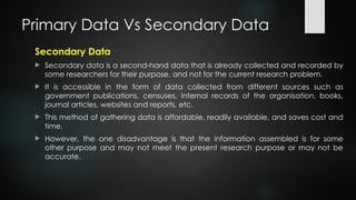
Secondary Data
Secondary data is a second-hand data that is already collected and recorded by
some researchers for their purpose, and not for the current research problem.
It is accessible in the form of data collected from different sources such as
government publications, censuses, internal records of the organisation, books,
journal articles, websites and reports, etc.
This method of gathering data is affordable, readily available, and saves cost and
time.
However, the one disadvantage is that the information assembled is for some
other purpose and may not meet the present research purpose or may not be
accurate.
7.
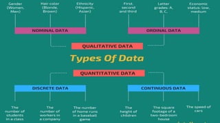
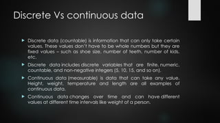
Discrete Vs continuousdata
Discrete data (countable) is information that can only take certain
values. These values don’t have to be whole numbers but they are
fixed values – such as shoe size, number of teeth, number of kids,
etc.
Discrete data includes discrete variables that are finite, numeric,
countable, and non-negative integers (5, 10, 15, and so on).
Continuous data (measurable) is data that can take any value.
Height, weight, temperature and length are all examples of
continuous data.
Continuous data changes over time and can have different
values at different time intervals like weight of a person.
8.
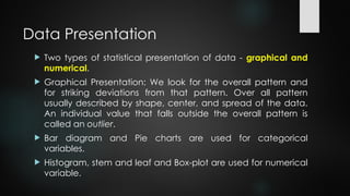
Data Presentation
Twotypes of statistical presentation of data - graphical and
numerical.
Graphical Presentation: We look for the overall pattern and
for striking deviations from that pattern. Over all pattern
usually described by shape, center, and spread of the data.
An individual value that falls outside the overall pattern is
called an outlier.
Bar diagram and Pie charts are used for categorical
variables.
Histogram, stem and leaf and Box-plot are used for numerical
variable.
9.
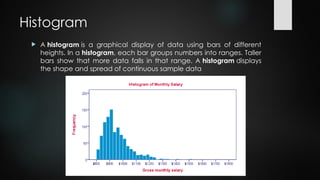
Histogram
A histogramis a graphical display of data using bars of different
heights. In a histogram, each bar groups numbers into ranges. Taller
bars show that more data falls in that range. A histogram displays
the shape and spread of continuous sample data
10.
Box Plotting
Boxplots (also called box-and-whisker plots or box-
whisker plots) give a good graphical image of the
concentration of the data.
They also show how far the extreme values are from most
of the data.
A box plot is constructed from five values: the minimum
value, the first quartile, the median, the third quartile, and
the maximum value.
11.
Box Plotting
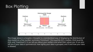
The imageabove is a boxplot. A boxplot is a standardized way of displaying the distribution of
data based on a five number summary (“minimum”, first quartile (Q1), median, third quartile
(Q3), and “maximum”). It can tell you about your outliers and what their values are. It can also
tell you if your data is symmetrical, how tightly your data is grouped, and if and how your data
is skewed.
12.
Statistical concepts ofclassification
of Data
Classification is the process of arranging data into homogeneous
(similar) groups according to their common characteristics.
Raw data cannot be easily understood, and it is not fit for further
analysis and interpretation. Arrangement of data helps users in
comparison and analysis. It is also important for statistical
sampling.
13.
Classification of Data
Thereare four types of classification. They are:
Geographical classification
When data are classified on the basis of location or areas, it is called geographical
classification
Chronological classification
Chronological classification means classification on the basis of time, like months,
years etc.
Qualitative classification
In Qualitative classification, data are classified on the basis of some attributes or
quality such as gender, colour of hair, literacy and religion. In this type of
classification, the attribute under study cannot be measured. It can only be found
out whether it is present or absent in the units of study.
Quantitative classification
Quantitative classification refers to the classification of data according to some
characteristics, which can be measured such as height, weight, income, profits etc.
14.
Quantitative classification
Thereare two types of quantitative classification of data: Discrete
frequency distribution and Continuous frequency distribution.
In this type of classification there are two elements
variable
Variable refers to the characteristic that varies in magnitude or quantity.
E.g. weight of the students. A variable may be discrete or continuous.
Frequency
Frequency refers to the number of times each variable gets repeated. For
example there are 50 students having weight of 60 kgs. Here 50 students is
the frequency.
15.
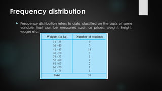
Frequency distribution
Frequencydistribution refers to data classified on the basis of some
variable that can be measured such as prices, weight, height,
wages etc.
16.
Frequency distribution
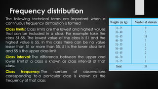
The followingtechnical terms are important when a
continuous frequency distribution is formed
Class limits: Class limits are the lowest and highest values
that can be included in a class. For example take the
class 51-55. The lowest value of the class is 51 and the
highest value is 55. In this class there can be no value
lesser than 51 or more than 55. 51 is the lower class limit
and 55 is the upper class limit.
Class interval: The difference between the upper and
lower limit of a class is known as class interval of that
class.
Class frequency: The number of observations
corresponding to a particular class is known as the
frequency of that class
17.
Measures of CentreTendency
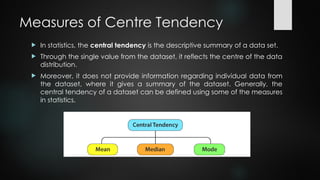
In statistics, the central tendency is the descriptive summary of a data set.
Through the single value from the dataset, it reflects the centre of the data
distribution.
Moreover, it does not provide information regarding individual data from
the dataset, where it gives a summary of the dataset. Generally, the
central tendency of a dataset can be defined using some of the measures
in statistics.
18.
Mean
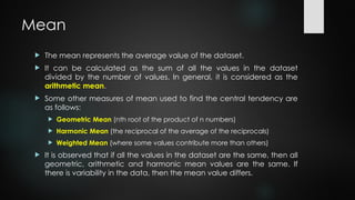
The meanrepresents the average value of the dataset.
It can be calculated as the sum of all the values in the dataset
divided by the number of values. In general, it is considered as the
arithmetic mean.
Some other measures of mean used to find the central tendency are
as follows:
Geometric Mean (nth root of the product of n numbers)
Harmonic Mean (the reciprocal of the average of the reciprocals)
Weighted Mean (where some values contribute more than others)
It is observed that if all the values in the dataset are the same, then all
geometric, arithmetic and harmonic mean values are the same. If
there is variability in the data, then the mean value differs.
19.
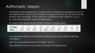
Arithmetic Mean
Arithmetic meanrepresents a number that is obtained by dividing the sum of
the elements of a set by the number of values in the set. So you can use the
layman term Average. If any data set consisting of the values b1, b2, b3, ….,
bn then the arithmetic mean B is defined as:
B = (Sum of all observations)/ (Total number of observation)
The arithmetic mean of Virat Kohli’s batting scores also called his Batting
Average is;
Sum of runs scored/Number of innings = 661/10
The arithmetic mean of his scores in the last 10 innings is 66.1.
20.
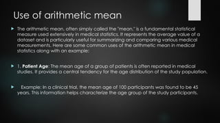
Use of arithmeticmean
The arithmetic mean, often simply called the "mean," is a fundamental statistical
measure used extensively in medical statistics. It represents the average value of a
dataset and is particularly useful for summarizing and comparing various medical
measurements. Here are some common uses of the arithmetic mean in medical
statistics along with an example:
1. Patient Age: The mean age of a group of patients is often reported in medical
studies. It provides a central tendency for the age distribution of the study population.
Example: In a clinical trial, the mean age of 100 participants was found to be 45
years. This information helps characterize the age group of the study participants.
21.
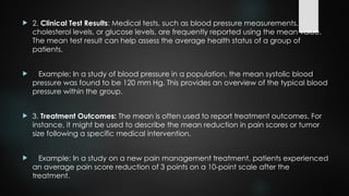
2. ClinicalTest Results: Medical tests, such as blood pressure measurements,
cholesterol levels, or glucose levels, are frequently reported using the mean value.
The mean test result can help assess the average health status of a group of
patients.
Example: In a study of blood pressure in a population, the mean systolic blood
pressure was found to be 120 mm Hg. This provides an overview of the typical blood
pressure within the group.
3. Treatment Outcomes: The mean is often used to report treatment outcomes. For
instance, it might be used to describe the mean reduction in pain scores or tumor
size following a specific medical intervention.
Example: In a study on a new pain management treatment, patients experienced
an average pain score reduction of 3 points on a 10-point scale after the
treatment.
22.
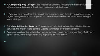
4. ComparingDrug Dosages: The mean can be used to compare the effectiveness of
different drug dosages or treatment regimens in clinical trials.
Example: In a drug trial, the mean improvement in lung function in patients taking a
higher dosage was 10% compared to a mean improvement of 5% in those taking a
lower dosage.
5. Patient Satisfaction Surveys: When patients rate their satisfaction with healthcare
services, the mean score can be used to summarize overall satisfaction.
Example: In a hospital satisfaction survey, patients gave an average rating of 4.2 on a
5point scale, indicating a relatively high level of satisfaction.
23.
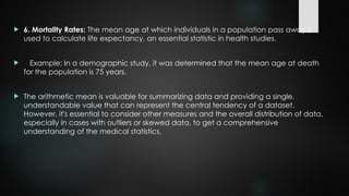
6. MortalityRates: The mean age at which individuals in a population pass away is
used to calculate life expectancy, an essential statistic in health studies.
Example: In a demographic study, it was determined that the mean age at death
for the population is 75 years.
The arithmetic mean is valuable for summarizing data and providing a single,
understandable value that can represent the central tendency of a dataset.
However, it's essential to consider other measures and the overall distribution of data,
especially in cases with outliers or skewed data, to get a comprehensive
understanding of the medical statistics.
24.
Harmonic Mean
A HarmonicProgression is a sequence if the reciprocals of its terms are in Arithmetic
Progression, and harmonic mean (or shortly written as HM) can be calculated by
dividing the number of terms by reciprocals of its terms.
In particular cases, especially those involving rates and ratios, the harmonic mean
gives the most correct value of the mean. For example, if a vehicle travels a
specified distance at speed x (eg 60 km / h) and then travels again at the speed y
(e.g.40 km / h), the average speed value is the harmonic mean x, y (Ie, 48 km / h).
25.
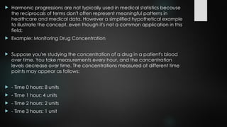
Harmonic progressionsare not typically used in medical statistics because
the reciprocals of terms don't often represent meaningful patterns in
healthcare and medical data. However a simplified hypothetical example
to illustrate the concept, even though it's not a common application in this
field:
Example: Monitoring Drug Concentration
Suppose you're studying the concentration of a drug in a patient's blood
over time. You take measurements every hour, and the concentration
levels decrease over time. The concentrations measured at different time
points may appear as follows:
- Time 0 hours: 8 units
- Time 1 hour: 4 units
- Time 2 hours: 2 units
- Time 3 hours: 1 unit
26.
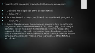
To analyzethis data using a hypothetical harmonic progression:
1. Calculate the reciprocals of the concentrations:
- 1/8,1/4,1/2,1/1
2. Examine the reciprocals to see if they form an arithmetic progression:
- 1/8,1/4,1/2,1/1
In this contrived example, the reciprocals appear to form an arithmetic
progression, with a common difference of ( frac{1}{8} ), indicating a
consistent rate of increase in the reciprocals. However, this specific
approach of using harmonic progressions to analyze drug concentration
data is not standard in medical statistics. More common methods involve
using exponential decay models, linear regression, or other statistical
techniques.
27.
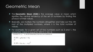
Geometric Mean
TheGeometric Mean (GM) is the average value or mean which
signifies the central tendency of the set of numbers by finding the
product of their values.
Basically, we multiply the numbers altogether and take out the nth
root of the multiplied numbers, where n is the total number of
values.
For example: for a given set of two numbers such as 3 and 1, the
geometric mean is equal to √(3+1) = √4 = 2.
28.
Use of GeometricMean
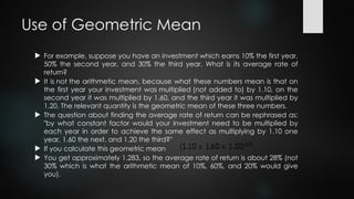
For example, suppose you have an investment which earns 10% the first year,
50% the second year, and 30% the third year. What is its average rate of
return?
It is not the arithmetic mean, because what these numbers mean is that on
the first year your investment was multiplied (not added to) by 1.10, on the
second year it was multiplied by 1.60, and the third year it was multiplied by
1.20. The relevant quantity is the geometric mean of these three numbers.
The question about finding the average rate of return can be rephrased as:
"by what constant factor would your investment need to be multiplied by
each year in order to achieve the same effect as multiplying by 1.10 one
year, 1.60 the next, and 1.20 the third?"
If you calculate this geometric mean
You get approximately 1.283, so the average rate of return is about 28% (not
30% which is what the arithmetic mean of 10%, 60%, and 20% would give
you).
29.
Certainly, let'sconsider an example of the use of the geometric
mean in the context of medical statistics:
Example: Disease Incidence Rates
Imagine a medical researcher is studying the incidence rates of a
rare infectious disease in two different regions over a period of three
years. The annual incidence rates (per 100,000 population) are as
follows:
- Region A:
- Year 1: 5 cases
- Year 2: 10 cases
- Year 3: 15 cases
30.
- RegionB:
- Year 1: 50 cases
- Year 2: 60 cases
- Year 3: 70 cases
The researcher wants to compare the average annual growth rate
of the disease incidence between these two regions. Since the
data represents rates and follows an exponential growth pattern,
the geometric mean is suitable for this analysis.
31.
To calculatethe geometric mean of the annual incidence rates for each
region:
For Region A:
1. Calculate the rate ratios: (10/5) *(15/10) = 3 *1.5 = 4.5.
2. Find the geometric mean of these rate ratios: 3√{4.5 *4.5 *4.5} ≈ 1.41/3
≈ 3.
For Region B:
1. Calculate the rate ratios: (60/50) *(70/60) = 1.2 *1.1667 ≈ 1.4
2. Find the geometric mean of these rate ratios: 3√{1.4 *1.4 *1.4} ≈ 1.41/3
≈
1.167.
32.
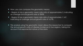
Now, youcan compare the geometric means:
- Region A has a geometric mean rate ratio of approximately 3, indicating
an average annual growth rate of 200%.
- Region B has a geometric mean rate ratio of approximately 1.167,
indicating an average annual growth rate of 16.7%.
This analysis using the geometric mean allows the researcher to compare
the annual growth rates of disease incidence in two regions, taking into
account the exponential nature of the data.
33.
Median
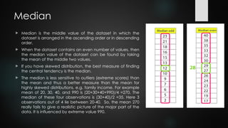
Median isthe middle value of the dataset in which the
dataset is arranged in the ascending order or in descending
order.
When the dataset contains an even number of values, then
the median value of the dataset can be found by taking
the mean of the middle two values.
If you have skewed distribution, the best measure of finding
the central tendency is the median.
The median is less sensitive to outliers (extreme scores) than
the mean and thus a better measure than the mean for
highly skewed distributions, e.g. family income. For example
mean of 20, 30, 40, and 990 is (20+30+40+990)/4 =270. The
median of these four observations is (30+40)/2 =35. Here 3
observations out of 4 lie between 20-40. So, the mean 270
really fails to give a realistic picture of the major part of the
data. It is influenced by extreme value 990.
34.
The medianis a crucial statistical measure used in medical statistics for a variety of
purposes, particularly when dealing with healthcare data. It represents the middle
value in a dataset when the data is ordered, and it's especially useful in cases where
extreme values or outliers may skew the data. Here are some common uses of the
median in medical statistics along with examples:
1. Patient Age: The median age of patients is often reported in medical studies. It is a
robust measure of central tendency and is less affected by outliers compared to the
mean.
Example: In a study of a group of patients, the median age is 47 years. This information
helps describe the middle value of the age distribution of the study population.
2. Pain Scores: In pain management and clinical trials, the median pain score can be a
more representative measure than the mean, especially when there are extreme pain
scores.
Example: In a clinical trial, the median pain score after a treatment is 3 on a 0-10
scale. This suggests that half of the patients experienced pain scores at or below 3.
35.
3. SurvivalTime: The median survival time is used to describe the time it takes for half of
a group of patients to reach a specific outcome, such as disease progression or death.
Example: In a study of patients with a certain cancer, the median survival time after
diagnosis is 24 months, indicating that half of the patients survived for at least 24
months.
4. Response to Treatment: The median can be used to assess how long it takes for a
particular treatment to show an effect in terms of patient response or disease
improvement.
Example: In a clinical trial for a new cancer drug, the median time to tumor shrinkage
was 8 weeks, indicating that half of the patients experienced tumor shrinkage within
that timeframe.
36.
5. WaitingTimes: In healthcare management, the median wait time for appointments,
surgeries, or emergency room visits can be essential to assess patient access and
service quality.
Example: In a hospital's emergency department, the median wait time for non-urgent
cases is 20 minutes, showing that half of the patients are seen within this time.
6. Disease Progression: When monitoring disease progression over time, the median
time it takes for the condition to worsen significantly can be a critical endpoint.
Example: In a study of Alzheimer's disease, the median time it takes for a patient's
cognitive function to deteriorate to a certain level is 3 years.
The median is particularly valuable in medical statistics when dealing with skewed data
or data with outliers because it reflects the middle value, which can be more
representative of the typical condition or outcome in a population. It is often used
alongside other measures like the mean and standard deviation to provide a
comprehensive understanding of the data.
37.
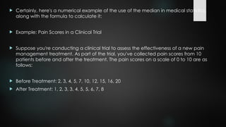
Certainly, here'sa numerical example of the use of the median in medical statistics,
along with the formula to calculate it:
Example: Pain Scores in a Clinical Trial
Suppose you're conducting a clinical trial to assess the effectiveness of a new pain
management treatment. As part of the trial, you've collected pain scores from 10
patients before and after the treatment. The pain scores on a scale of 0 to 10 are as
follows:
Before Treatment: 2, 3, 4, 5, 7, 10, 12, 15, 16, 20
After Treatment: 1, 2, 3, 3, 4, 5, 5, 6, 7, 8
38.
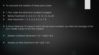
To calculatethe median of these pain scores:
1. First, order the data from smallest to largest:
Before Treatment: 2, 3, 4, 5, 7, 10, 12, 15, 16, 20
After Treatment: 1, 2, 3, 3, 4, 5, 5, 6, 7, 8
2. Since there are 10 values in each set (an even number), you take the average of the
two middle values to find the median:
Median of Before Treatment = {7 + 10}/2 = 8.5
Median of After Treatment ={4 + 5}/2 = 4.5
39.
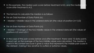
In thisexample, the median pain score before treatment is 8.5, and the median pain
score after treatment is 4.5.
The formula to calculate the median is as follows:
For an Odd Number of Data Points (n):
- Median = Middle value in the ordered data set (the value at position (n+1)/2)
For an Even Number of Data Points (n):
- Median = Average of the two middle values in the ordered data set (the values at
positions n/2 and n/2+1
In the case of the pain scores before and after treatment, there were 10 data points
in each set, so the average of the two middle values was calculated. The median is
useful in this context because it gives a value that represents the middle pain score in
the dataset, making it less sensitive to outliers or extreme values.
40.
Mode
The moderepresents the frequently occurring value in the
dataset.
Sometimes the dataset may contain multiple modes and in
some cases, it does not contain any mode at all.
If you have categorical data, the mode is the best choice
to find the central tendency.
41.
Use of Modes
The mode is a statistical measure used in medical statistics and healthcare research to
identify the most frequently occurring value in a dataset. It can provide valuable
insights in various medical and clinical scenarios. Here are some common uses of the
mode in medical statistics, along with examples:
1. Patient Blood Type: The mode is used to determine the most common blood type in
a population, which is essential for blood transfusions and organ transplant
compatibility.
Example: In a study of 500 patients, blood type A+ was the most common, occurring
in 250 patients.
42.
2. MedicationDosage: In pharmacology and medication management, the mode
can help identify the most commonly prescribed or administered dosage for a
specific drug.
Example: Among 100 patients receiving a particular pain medication, the most
common dosage prescribed was 10 mg.
3. Symptom Severity: In patient assessment and symptom tracking, the mode can be
used to identify the most frequently reported symptom severity or intensity.
Example: In a study of COVID-19 patients, the most common symptom severity was
mild, reported by 80% of the patients.
43.
4. PatientSatisfaction Ratings: Patient satisfaction surveys often use the mode to identify
the most common rating or feedback given by patients regarding healthcare services.
Example: In a hospital satisfaction survey, the mode satisfaction rating was 5 on a 5-
point scale, indicating that most patients were highly satisfied.
5. Pain Intensity: The mode can be used to identify the most frequently reported pain
intensity level in clinical pain assessments.
Example: In a study of post-operative patients, moderate pain (rated as 5 on a scale
from 0 to 10) was the most frequently reported pain intensity level.
6
44.
. Frequencyof Adverse Events: The mode is used to determine the most common
adverse events or side effects associated with a specific treatment or medication.
Example: In a drug trial, the most frequently reported adverse event was mild dizziness,
occurring in 30% of the patients.
The mode is valuable in medical statistics for identifying prevalent categories or values,
which can be critical for clinical decision-making, resource allocation, and patient
management. However, it's important to note that the mode may not always exist in a
dataset, or there may be multiple modes when multiple values occur with the same
highest frequency. In such cases, the dataset is described as "multimodal."


![[DSC Europe 25] Ivan Lukovic & Marija Djukic - From Data to Value: Why Maturi...](https://cdn.slidesharecdn.com/ss_thumbnails/ahrfps8xr6knowwhacxh-1-ivan-marija-dsc-2025-ld-v1-presentation-260115093812-be21adfc-thumbnail.jpg?width=640&height=640&fit=bounds)


![[DSC Europe 25] Bojan Djuricic - Predictive Design Process.pdf](https://cdn.slidesharecdn.com/ss_thumbnails/5awdrbedqdek3gqu2ezy-4-the-predictive-design-bojan-djuricic-260120105856-6c399e9b-thumbnail.jpg?width=640&height=640&fit=bounds)


