This document discusses reproducible research with RStudio and knitr. It introduces literate programming with knitr, which allows code chunks to be embedded within LaTeX documents. RStudio provides a convenient graphical user interface for knitr by compiling documents with a single button click. The document provides examples of embedding R code and graphics within LaTeX and discusses various knitr chunk options for controlling code evaluation and output.

1. Introduction
Details
Reproducible research with RStudio and knitr
Ben Bolker
McMaster University, Mathematics & Statistics and Biology
25 February 2014
Ben Bolker
RStudio and knitr

2. Introduction
Details
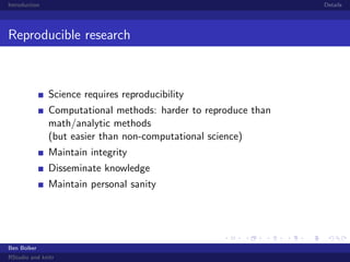
Reproducible research
Science requires reproducibility
Computational methods: harder to reproduce than
math/analytic methods
(but easier than non-computational science)
Maintain integrity
Disseminate knowledge
Maintain personal sanity
Ben Bolker
RStudio and knitr

3. Introduction
Details
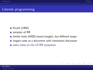
Literate programming
Knuth (1984)
ancestor of RR
similar tools (WEB/weave/tangle), but different scope
targets code as a document with interwoven discussion
some notes on the LP-RR ecosystem
Ben Bolker
RStudio and knitr

4. Introduction
Details
A
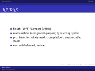
TEX/LTEX
Knuth (1978)/Lamport (1980s)
mathematical (and general-purpose) typesetting system
pro: beautiful, widely used, cross-platform, customizable,
stable
con: old-fashioned, arcane
Ben Bolker
RStudio and knitr

5. Introduction
Details
R
Gentleman and Ihaka, 1990s
statistical programming language/data analysis environment
pro: powerful, widely used (3000+ packages), cross-platform,
customizable
con: slower than low-level languages; organic/inconsistent
Ben Bolker
RStudio and knitr

6. Introduction
Details
Sweave/knitr
Leisch / Xie
A
literate programming tool, allowing LTEX chunks in R
highlighted code chunks (echo=TRUE)
automatically generated figures, optionally in a figure
environment
pro: super-convenient, once you get used to it
con: one more software layer;
not suited for big projects/code
Ben Bolker
RStudio and knitr

7. Introduction
Details
RStudio
Allaire et al.
front-end for R
one-button front end for knitr (“Compile PDF”)
pro: beginner-friendly; cross-platform;
zoomable graphics, code highlighting, tab completion,
environment listing, etc.
con: R-centric; restriction to built-in editor;
one more software layer
Ben Bolker
RStudio and knitr

8. Introduction
Details
Getting started
bookmark the knitr web page and especially the options page
switch RStudio to compile documents with knitr
(Tools/Global options/Sweave/Weave Rnw files using ...)
A
make sure LTEX is installed/working and the knitr package
is installed (install.packages("knitr")); also install
tikzDevice package
build this document, or use (File/New File/R Sweave) to
generate an empty template (need to add something to it);
RStudio recognizes .Rnw extension
code chunks start with <<>>= and end with @
Ben Bolker
RStudio and knitr

9. Introduction
Details
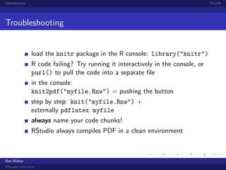
Troubleshooting
load the knitr package in the R console: library("knitr")
R code failing? Try running it interactively in the console, or
purl() to pull the code into a separate file
in the console:
knit2pdf("myfile.Rnw") = pushing the button
step by step: knit("myfile.Rnw") +
externally pdflatex myfile
always name your code chunks!
RStudio always compiles PDF in a clean environment
Ben Bolker
RStudio and knitr

10. Introduction
Details
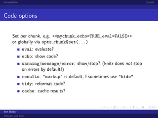
Code options
Set per chunk, e.g. <<mychunk,echo=TRUE,eval=FALSE>>
or globally via opts chunk$set(...)
eval: evaluate?
echo: show code?
warning/message/error: show/stop? (knitr does not stop
on errors by default!)
results: "markup" is default, I sometimes use "hide"
tidy: reformat code?
cache: cache results?
Ben Bolker
RStudio and knitr

11. Introduction
Details
More stuff about code
if you’re using beamer, need to use
begin{frame}[fragile] if you’re going to show code (i.e.,
echo=TRUE)
code in chunks must be complete/syntactically correct: no
fragments allowed;
can’t (e.g.) separate parts of a for loop, even if eval=FALSE
in-line expressions via Sexpr{} (don’t forget to round
numeric values)
Ben Bolker
RStudio and knitr

12. Introduction
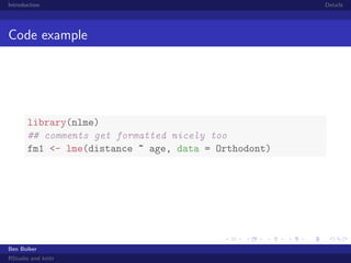
Code example
library(nlme)
## comments get formatted nicely too
fm1 <- lme(distance ~ age, data = Orthodont)
Ben Bolker
RStudio and knitr
Details

13. Introduction
Details
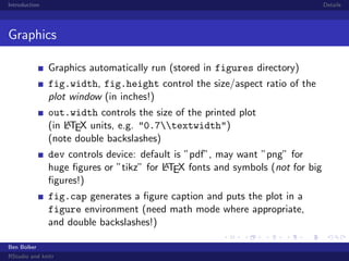
Graphics
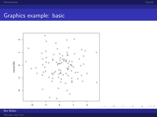
Graphics automatically run (stored in figures directory)
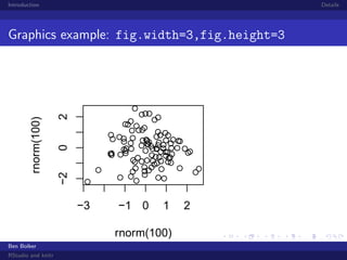
fig.width, fig.height control the size/aspect ratio of the
plot window (in inches!)
out.width controls the size of the printed plot
A
(in LTEX units, e.g. "0.7textwidth")
(note double backslashes)
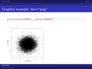
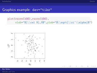
dev controls device: default is ”pdf”, may want ”png” for
A
huge figures or ”tikz” for LTEX fonts and symbols (not for big
figures!)
fig.cap generates a figure caption and puts the plot in a
figure environment (need math mode where appropriate,
and double backslashes!)
Ben Bolker
RStudio and knitr

14. Introduction
Details
0
−2
−1
rnorm(100)
1
2
Graphics example: basic
−2
Ben Bolker
RStudio and knitr
−1
0
rnorm(100)
1
2

15. Introduction
Details
2
0
−2
rnorm(100)
Graphics example: fig.width=3,fig.height=3
−3
−1 0
1
rnorm(100)
Ben Bolker
RStudio and knitr
2

16. Introduction
Details
Graphics example: dev="png"
0
−2
rnorm(10000)
2
4
plot(rnorm(10000), rnorm(10000))
−4
−2
0
rnorm(10000)
Ben Bolker
RStudio and knitr
2
4

17. Introduction
Details
Graphics example: dev="tikz"
0
-2
-1
√
ξα
1
2
plot(rnorm(100),rnorm(100),
xlab="${cal R}_0$",ylab="$sqrt{xi^alpha}$")
-3
-2
-1
0
R0
Ben Bolker
RStudio and knitr
1
2
3

18. Introduction
Details
Other stuff
other input formats: R markdown
chunks in other languages
output to other formats: HTML, docx
other ways of documenting/disseminating results:
commented R code (spin()); R packages/vignettes;
roxygen2 package
large/batch jobs: caching gets tricky, use Makefiles instead?
figure tricks: 3D (rgl) plots, animation . . .
Ben Bolker
RStudio and knitr

19. Introduction
Details
Further resources
knitr web page, including the demos and showcase . . .
StackOverflow
my examples on Rpubs
knitr book on Amazon
Ben Bolker
RStudio and knitr