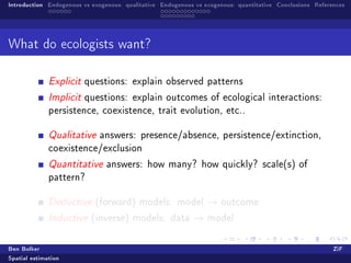
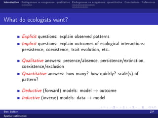
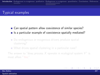
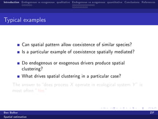
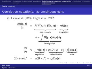
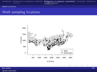
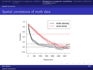
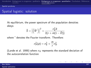
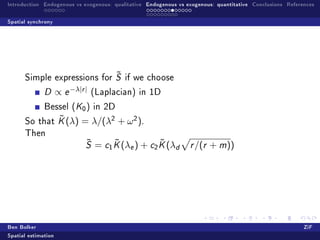
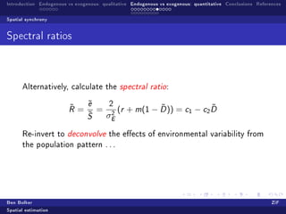
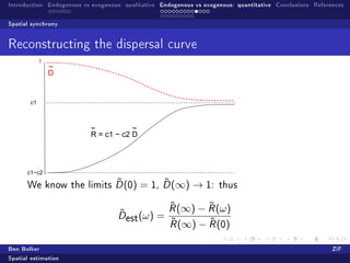
Introduction Endogenous vs exogenous: qualitative Endogenous vs exogenous: quantitative Conclusions References


               Estimating environmental heterogeneity from
                                   spatial dynamics data


                               Ben Bolker, McMaster University
                             Departments of Mathematics & Statistics and Biology


                                                    ZiF


                                             18 June 2012


Ben Bolker                                                                                                ZiF
Spatial estimation
Introduction Endogenous vs exogenous: qualitative Endogenous vs exogenous: quantitative Conclusions References


Outline


       1   Introduction


       2   Endogenous vs exogenous: qualitative
               Explanations for spatial patterns


       3   Endogenous vs exogenous: quantitative
               Spatial synchrony
               Pines


       4   Conclusions


Ben Bolker                                                                                                ZiF
Spatial estimation
Introduction Endogenous vs exogenous: qualitative Endogenous vs exogenous: quantitative Conclusions References


What do ecologists want?


              Explicit questions: explain observed patterns

              Implicit questions: explain outcomes of ecological interactions:
              persistence, coexistence, trait evolution, etc..


              Qualitative answers: presence/absence, persistence/extinction,
              coexistence/exclusion

              Quantitative answers: how many? how quickly? scale(s) of
              pattern?


              Deductive (forward) models: model                  →   outcome

              Inductive (inverse) models: data              →    model


Ben Bolker                                                                                                ZiF
Spatial estimation
Introduction Endogenous vs exogenous: qualitative Endogenous vs exogenous: quantitative Conclusions References


Typical examples


              Can spatial pattern allow coexistence of similar species?

              Is a particular example of coexistence spatially mediated?


              Do endogenous or exogenous drivers produce spatial
              clustering?

              What drives spatial clustering in a particular case?

      The answer to does process X operate in ecological system Y  is
      most often  Yes.


Ben Bolker                                                                                                ZiF
Spatial estimation
Introduction Endogenous vs exogenous: qualitative Endogenous vs exogenous: quantitative Conclusions References


Typical models


              Stochastic spatial point processes: continuous time  space,
              point individuals, innite domains

              Spatial (two-point, truncated) correlation functions

              Usually assume isotropy and translational invariance

              Exogenous heterogeneity expressed as correlation function of
              parameters

      e.g. spatial logistic:
        Process             Eect                                             Rate
                                                                                      −
        competition         subtract individual at x                 x ∈γ     y ∈γ a (y − x )
        death               subtract point at x                              x ∈γ m(x )
                                                                                +
        birth               add point at x
                                                                   Ω      y ∈γ a (y − x ) dx
Ben Bolker                                                                                                ZiF
Spatial estimation
Introduction Endogenous vs exogenous: qualitative Endogenous vs exogenous: quantitative Conclusions References

Explanations for spatial patterns


Outline


       1   Introduction


       2   Endogenous vs exogenous: qualitative
               Explanations for spatial patterns


       3   Endogenous vs exogenous: quantitative
               Spatial synchrony
               Pines


       4   Conclusions


Ben Bolker                                                                                                ZiF
Spatial estimation
Introduction Endogenous vs exogenous: qualitative Endogenous vs exogenous: quantitative Conclusions References

Explanations for spatial patterns


Templates


           assume habitat map reects
           underlying spatial pattern
           more or less exactly: low
           diusion (but             0),   high
           growth rate
                                                                         photo: Henry Horn


Ben Bolker                                                                                                ZiF
Spatial estimation
Introduction Endogenous vs exogenous: qualitative Endogenous vs exogenous: quantitative Conclusions References

Explanations for spatial patterns


Nonlinear (deterministic) pattern formation


           Turing instabilities: unstable
           spatial modes of nonlinear
           systems

           in ecology: tiger bush,
           spruce waves, predator-prey
           spirals    (Rohani et al., 1997)
           requires no noise, just initial
           perturbation
                                                                       tiger bush (Wikipedia)


Ben Bolker                                                                                                ZiF
Spatial estimation
Introduction Endogenous vs exogenous: qualitative Endogenous vs exogenous: quantitative Conclusions References

Explanations for spatial patterns


Demographic noise-driven pattern

              Correlation equations: Dirac            δ   function in spatial correlation
              function due to discreteness

              Drives pattern in homogeneous, stable systems (e.g.
              competition): C        =0    is not even an equilibrium for the spatial
              logistic equation
              Eects could be weak:
                      depend on scale of interaction neighborhood (Bolker, 1999): in
                      numbers of individuals: ≈ 10, 100, 1000 ?
                      eects depend on R = f /µ for equal scale of dispersal 
                      competition, get even pattern if R  2 (Bolker  Pacala,
                      1999)
              Could be stronger with ne-scale heterogeneity (e.g. negative
              binomial noise?)

Ben Bolker                                                                                                ZiF
Spatial estimation
Introduction Endogenous vs exogenous: qualitative Endogenous vs exogenous: quantitative Conclusions References

Explanations for spatial patterns


General (environmental) noise-driven pattern


      Most general case: space(-time) noise                  ξ(x , t , N (t ))
              Scale may be          0   (non-white in space and time)
                                                                   √
              Amplitude may scale dierently from                      N

              Space-time correlations:
                      separable Snyder  Chesson (2004) ?
                      other correlations can be framed as outcomes of dynamical
                      processes
      Properties other than 2-point correlation functions?


Ben Bolker                                                                                                ZiF
Spatial estimation
Introduction Endogenous vs exogenous: qualitative Endogenous vs exogenous: quantitative Conclusions References

Explanations for spatial patterns


Summary: what do we need?


              Lots of interesting questions, but perhaps existing methods are
              good enough for ecologists?

              Importance of stochastic dynamics at various scales:
                      Is demographic (endogenous) noise really that important?
                      Perhaps a more traditional separation of scales (individual,
                      patch, site, . . . ) is enough?
              How do we estimate the (eects of) heterogeneity?


Ben Bolker                                                                                                ZiF
Spatial estimation
Introduction Endogenous vs exogenous: qualitative Endogenous vs exogenous: quantitative Conclusions References

Spatial synchrony


Outline


       1   Introduction


       2   Endogenous vs exogenous: qualitative
               Explanations for spatial patterns


       3   Endogenous vs exogenous: quantitative
               Spatial synchrony
               Pines


       4   Conclusions


Ben Bolker                                                                                                ZiF
Spatial estimation
Introduction Endogenous vs exogenous: qualitative Endogenous vs exogenous: quantitative Conclusions References

Spatial synchrony


Spatial synchrony


           Eastern spruce budworm,
           Choristeroneura fumiferna

           non-spatial dynamics: plant
           quality, climate, enemies
           (Kendall et al., 1999)?
           What generates large-scale
           spatial synchrony?
                     Moran eect: large-scale
                     weather patterns
                     Dispersal coupling:
                     movement of larvae

Ben Bolker                                                                                                ZiF
Spatial estimation
Introduction Endogenous vs exogenous: qualitative Endogenous vs exogenous: quantitative Conclusions References

Spatial synchrony


Correlation equations:                   via continuous eqns
      cf.   Lande et al. (1999),       Engen et al. 2002:


                     ∂ N (x, t )
                                   =    F (N (  x, t ), E (x, t )) −   mN (   x)
                        ∂t
                                              pop. growth              emigration


                                         +m        D(   y, x)N (y) d y
                                                      immigration


                            ∂n
                                   ≈ −rn(x, t ) + m(D ∗ n − n) + σE e (x, t )
                                                                  2

                            ∂t
                                         regulation        redistribution           noise

                              ∗                     ∗        2
                2(r   + m)c        =    m (D   ∗ c ) + σE Cor(e )

Ben Bolker                                                                                                ZiF
Spatial estimation
Introduction Endogenous vs exogenous: qualitative Endogenous vs exogenous: quantitative Conclusions References

Spatial synchrony


Moth sampling locations


                                2000
                                                                                                    q
                                                                                                    q q
                                       q q                                                            q      q   q
                                       q q q q                                                        q      q   q q q
                                1500   q q q     q q                                      q    q q qq q
                                                                                                      q      q   q q q q
                                       q q       q                                q q q q q qq q q q
                                                                                               q           qqq     q
                                                                                                                 q q q q
                     N−S (km)


                                       q q q q q                    q q      q q q q q q q q qqq q q        q
                                                                                                           q q   q   q
                                       q q q q q q q             q qqq q q q q q qq q qq q qqq q
                                                                                      q     q     q        q q
                                                                                      q
                                       q q q q q qq q
                                                   q                 q                  qq
                                                         q q q q q q qqq q q q qqq qq q q qq q q q q q
                                                                                          qq
                                                                                          q       q    q
                                1000     q
                                       q qq q q q q q
                                                     q                      q             qq
                                                         q q q q q q q q q q q q qq qq q q q q qq q q q
                                                                       qq
                                                                                                          q
                                          qq q q q q
                                             q
                                           q q              q    q            q       q q q
                                                                                          q
                                                                                             q
                                                                                                  q   q q
                                                                                                      q
                                        qq
                                       q q q q q q q q   qq q q q q q q qqq q q q q q q qqqq q qq
                                                           q                          q q    q qq q
                                                                                                 q q     q
                                               q q qq
                                               q           q                               q      q   q
                                                 q q q   q q   q q q q q q q qqq qq qqq q q q q q q
                                                                        q q       q qq      q qq qq qq
                                                                                     q q
                                                                                     q q       q
                                                 qq q
                                                   q q
                                                   q     q q     q q qq             qqq
                                                                                            q
                                                                 q q q q qqq qq qq q q q q q q q
                                                                              q q qq q       q
                                                   q q             q q q qqqqq qq
                                                                    q     qq      q
                                                                                  qq        q q
                                500                                     q
                                                                        qq q q q
                                                                         q
                                                                        qq q qq
                                                                        qqqq
                                                                           q
                                                                        qq qq
                                                                          q
                                                                          q qq
                                                                          qq
                                                                        qq q q
                                                                          q
                                                                                                    q  SBW
                                   0                                                               q   temperature


                                            500      1000         1500        2000       2500       3000         3500

                                                                        E−W (km)


Ben Bolker                                                                                                                 ZiF
Spatial estimation
Introduction Endogenous vs exogenous: qualitative Endogenous vs exogenous: quantitative Conclusions References

Spatial synchrony


Moth dynamics


                                                q
                                                qq
                     qq               1945       q qq
          1500       qqqq                        q qqqq
                     qqq qq                 q qqqqq qqqqq                                     z

                     qq   q             qqqqqqqqqq qqqqqq                                     q 0.0
                     qqqqq        qq qqqqqqqqqqqq qqq q                                       q 0.2
                     qqqqqqq     qqqqqqqqqqqqqqqq qq
          1000       qqqqqqqqqqqqqqqqqqqqqqqqqqqqqqqq                                         q 0.4
                     qqqqqqqqqqqqqqqqqqqqqqqqqqqqqqqq                                         q 0.6
                     qqqqqqqqqqqqqqqqqqqqqqqqqqqqqq                                           q 0.8
                          qqqqq qqqqqqqqqqqqqqqqqq                                            q 1.0
                          qqqqq qqqqqqqqqqqqqqqq
           500             qq     qqqqqqqq   qq
                                    qqqqq
                                    qqq
                                    qqq
                 0              1000                 2000                3000


Ben Bolker                                                                                                ZiF
Spatial estimation
Introduction Endogenous vs exogenous: qualitative Endogenous vs exogenous: quantitative Conclusions References

Spatial synchrony


Spatial correlations of moth data


                                    1.0
                                                                           moth density
                                    0.8                                    June temp.

                                    0.6
                     Correlation


                                    0.4


                                    0.2


                                    0.0


                                   −0.2

                                          0   500   1000    1500    2000   2500   3000

                                                           Distance (km)


Ben Bolker                                                                                                ZiF
Spatial estimation
Introduction Endogenous vs exogenous: qualitative Endogenous vs exogenous: quantitative Conclusions References

Spatial synchrony


Spatial logistic: solution


      At equilibrium, the power spectrum of the population densities
      obeys
                                                                  2
                              ˜         ˜   ∗
                                                 2               σE e
                                                                    ˜
                              S   =     N            =
                                                         2(r           ˜
                                                               + m(1 − D ))
      where     ˜ denotes    the Fourier transform. Therefore:

                                         2         2
                                                                m    2
                                        σP (p ) = σE +              σD
                                                                r

      (Lande et al. 1999) where                 σX   represents the standard deviation of
      the autocorrelation function


Ben Bolker                                                                                                ZiF
Spatial estimation
Introduction Endogenous vs exogenous: qualitative Endogenous vs exogenous: quantitative Conclusions References

Spatial synchrony


                             ˜
      Simple expressions for S if we choose

              D      ∝ e −λ|r |   (Laplacian) in 1D

              Bessel (K0 ) in 2D
              ˜
      So that K (λ)          = λ/(λ2 + ω 2 ).
      Then
                              ˜
                              S        ˜            ˜
                                  = c1 K (λe ) + c2 K (λd        r /(r   + m))


Ben Bolker                                                                                                ZiF
Spatial estimation
Introduction Endogenous vs exogenous: qualitative Endogenous vs exogenous: quantitative Conclusions References

Spatial synchrony


Spectral ratios


      Alternatively, calculate the spectral ratio:


                        ˜       ˜
                                e        2
                                                        ˜              ˜
                        R   =       =        (r + m(1 − D )) = c1 − c2 D
                                ˜
                                S
                                         2
                                        σE

      Re-invert to deconvolve the eects of environmental variability from
      the population pattern . . .


Ben Bolker                                                                                                ZiF
Spatial estimation
Introduction Endogenous vs exogenous: qualitative Endogenous vs exogenous: quantitative Conclusions References

Spatial synchrony


Reconstructing the dispersal curve
            1
                ~
                D


       c1


                           ~           ~
                           R = c1 − c2 D


      c1−c2
                         ˜
      We know the limits D (0)                  ˜
                                           = 1, D (∞) → 1:           thus


                                                    ˜
                                                    R (∞)   ˜
                                                          − R (ω)
                                    ˜
                                    Dest (ω)    =
                                                    ˜       ˜
                                                    R (∞) − R (0)


Ben Bolker                                                                                                ZiF
Spatial estimation
Introduction Endogenous vs exogenous: qualitative Endogenous vs exogenous: quantitative Conclusions References

Spatial synchrony


Moth data: spectra


                                                                        Environment
                       Population
                         10000                                             2e+06


                             500

                                                                           1e+05
                                   0.000         0.010          0.020
                                        Frequency (km−1)

Ben Bolker                                                                                                ZiF
Spatial estimation
Introduction Endogenous vs exogenous: qualitative Endogenous vs exogenous: quantitative Conclusions References

Spatial synchrony


Moth data: spectral ratios


                             100

                             200
                     Ratio


                             300

                             400

                             500

                                   0.000       0.005         0.010          0.015
                                                                 −1
                                               Frequency (km )


Ben Bolker                                                                                                ZiF
Spatial estimation
Introduction Endogenous vs exogenous: qualitative Endogenous vs exogenous: quantitative Conclusions References

Spatial synchrony


(Putative) moth dispersal curve


                                 0.25


                                 0.20
                     Dispersal


                                 0.15


                                 0.10


                                 0.05


                                 0.00

                                        0   100   200        300      400       500

                                                   Distance (km)


Ben Bolker                                                                                                ZiF
Spatial estimation
Introduction Endogenous vs exogenous: qualitative Endogenous vs exogenous: quantitative Conclusions References

Pines


Outline


        1   Introduction


        2   Endogenous vs exogenous: qualitative
               Explanations for spatial patterns


        3   Endogenous vs exogenous: quantitative
               Spatial synchrony
               Pines


        4   Conclusions


Ben Bolker                                                                                                ZiF
Spatial estimation
Introduction Endogenous vs exogenous: qualitative Endogenous vs exogenous: quantitative Conclusions References

Pines


Pines


             Slash pine, Pinus elliottii

             Data on seed distribution,
             seedling distribution, but
             not collected on the same
             quadrats

             Sampling scheme highly
             irregular; sparse data


                                                          Wikipedia
Ben Bolker                                                                                                ZiF
Spatial estimation
Introduction Endogenous vs exogenous: qualitative Endogenous vs exogenous: quantitative Conclusions References

Pines


Seed data

                                     A                F                D
                        50
                        40
                        30
                        20
                        10                                                          empty
                         0                                                             TRUE
                                     B                E                G
                                                                                       FALSE
                        50
                        40                                                          count
                        30                                                             0
                        20
                                                                                       10
                        10
                         0                                                             20
                                     H                J                C               30
                        50                                                             40
                        40
                        30
                        20
                        10
                         0
                             0   10 20 30 40 50
                                              0   10 20 30 40 50
                                                               0   10 20 30 40 50


Ben Bolker                                                                                                ZiF
Spatial estimation
Introduction Endogenous vs exogenous: qualitative Endogenous vs exogenous: quantitative Conclusions References

Pines


Sapling data

                                  D             E          B       J
                        50
                        40
                        30                                                  empty
                        20
                                                                               TRUE
                        10
                                                                               FALSE
                         0
                                  A             F          H       G
                                                                            count
                        50
                                                                               0
                        40
                        30                                                     2
                        20                                                     4
                        10                                                     6
                         0
                                                                               8
                                  C             K
                                                                               10
                        50
                                                                               12
                        40
                        30                                                     14
                        20
                        10
                         0
                             0 102030405060 102030405060
                                          0


Ben Bolker                                                                                                ZiF
Spatial estimation
Introduction Endogenous vs exogenous: qualitative Endogenous vs exogenous: quantitative Conclusions References

Pines


Correlation functions

                                                      seedling                    seed
                                        1.0


                                        0.8
                      Autocorrelation


                                        0.6


                                        0.4


                                        0.2


                                        0.0
                                              0   5   10   15    20   25 0   5   10   15   20   25
                                                                 Distance (m)

Ben Bolker                                                                                                ZiF
Spatial estimation
Introduction Endogenous vs exogenous: qualitative Endogenous vs exogenous: quantitative Conclusions References

Pines


Analytical framework (2)

              assume cross-covariance C           EN = 0
              no correlation between seeds and environment,
              e.g. long-distance dispersal

                                  C           ¯
                                    SS (r ) = N
                                                   2
                                                       C             ¯
                                                           EE (r ) + E
                                                                         2
                                                                             NN (r )
                                                                             C

                     ¯                       ¯
              (where N =mean seed density, , E =mean establishment
              probability)

              or (switch to correlation c )

                                                                     2

                                                             EE + ¯N cNN
                                                  σ2E             σ
                                       C   SS ∝ ¯      2
                                                            c
                                                                     2
                                                E                 N

              . . . a weighted mixture of the two correlation functions

Ben Bolker                                                                                                ZiF
Spatial estimation
Introduction Endogenous vs exogenous: qualitative Endogenous vs exogenous: quantitative Conclusions References

Pines


Solving for          cEE


        Therefore,
                                    c              ¯
                                     EE ∝ σS cSS − E σN cNN
                                                2            2   2


        Can we really use this?


Ben Bolker                                                                                                ZiF
Spatial estimation
Introduction Endogenous vs exogenous: qualitative Endogenous vs exogenous: quantitative Conclusions References

Pines


Results: observed/inferred correlation equations

                                        seedling            seed                 env


                          1.0


                                                                                              w
        Autocorrelation


                                                                                                  est
                          0.5
                                                                                              type
                                                                                                 seedling
                                                                                                 seed
                                                                                                 env
                          0.0


                                0   5   10 15 20 25 0   5   10 15 20 25 0   5   10 15 20 25
                                                        Distance (m)
Ben Bolker                                                                                                  ZiF
Spatial estimation
Introduction Endogenous vs exogenous: qualitative Endogenous vs exogenous: quantitative Conclusions References

Pines


Simulation results

                                         seedling            seed                 env

                           1.0


                           0.8
                                                                                               type
        Autocorrelation


                                                                                                  seedling
                           0.6
                                                                                                  seed
                                                                                                  env
                           0.4
                                                                                               w
                                                                                                   true
                           0.2                                                                     est

                           0.0


                          −0.2
                                 0   5   10 15 20 25 0   5   10 15 20 25 0   5   10 15 20 25
                                                         Distance (m)
Ben Bolker                                                                                                   ZiF
Spatial estimation
Introduction Endogenous vs exogenous: qualitative Endogenous vs exogenous: quantitative Conclusions References


Caveats/assumptions


              Assumes linearization/moment truncation

              Assumes isotropy/homogeneity

              Estimating spectra of small, irregular, noisy data sets is
              dicult (!)

              Advantages vs. direct estimation (e.g. via MCMC) ?


Ben Bolker                                                                                                ZiF
Spatial estimation
Introduction Endogenous vs exogenous: qualitative Endogenous vs exogenous: quantitative Conclusions References


Goals


              Simple, light-weight (!!), non-parametric (??) approach to
              spatial estimation

              leverage unreasonable eectiveness of linearization
              (Gurney  Nisbet, 1998)
              Use all available information:
                     snapshots, before/after, time/series
                     non-matching spatial samples


Ben Bolker                                                                                                ZiF
Spatial estimation
Introduction Endogenous vs exogenous: qualitative Endogenous vs exogenous: quantitative Conclusions References


Acknowledgements


               People Ottar Bjørnstad, Sandy Liebhold, Aaron Berk, Gordon
                         Fox, Stephen Cornell, Mollie Brooks, Emilio Bruna

             Funding NSF, NSERC (Discovery Grant)


Ben Bolker                                                                                                ZiF
Spatial estimation
Introduction Endogenous vs exogenous: qualitative Endogenous vs exogenous: quantitative Conclusions References


Meta-issues


              Why do interdisciplinary work? Public vs. private explanations:


                     for fun
                     to nd interesting math problems
                     to solve biological problems (basic or applied)
                     career enhancement (publications, grants, publicity . . . )
              Interactions of science with mathematics
                     Physics vs. biology vs. social sciences
                     Quantitative or qualitative dierences?
                     Which dierences matter? Scale, noisiness, data
                     quality/quantity, culture (lumpers vs. splitters), . . . ?
                     Are dierent strategies required?

Ben Bolker                                                                                                ZiF
Spatial estimation
Introduction Endogenous vs exogenous: qualitative Endogenous vs exogenous: quantitative Conclusions References


      http://xkcd.com/435/


Ben Bolker                                                                                                ZiF
Spatial estimation
Introduction Endogenous vs exogenous: qualitative Endogenous vs exogenous: quantitative Conclusions References


      Bolker, BM, 1999. 61:849874.
      Bolker, BM  Pacala, SW, 1999. American Naturalist, 153:575602.
      Gurney, WSC  Nisbet, R, 1998. Ecological Dynamics. Oxford University Press, Oxford, UK. ISBN
         0195104439.
      Kendall, B, Briggs, C, Murdoch, W, et al., 1999. Ecology, 80:17891805.
      Lande, R, Engen, S,  Sæther, B, 1999. The American Naturalist, 154(3):271281.
         doi:10.1086/303240. URL http://dx.doi.org/10.1086/303240.
      Rohani, P, Lewis, TJ, Grunbaum, D, et al., 1997. Trends in Ecology  Evolution, 12(2):7074. ISSN
         0169-5347. doi:10.1016/S0169-5347(96)20103-X. URL http:
          //www.sciencedirect.com/science/article/B6VJ1-3X2B51F-19/2/752d6d91ad9282ab7ec3707fdf4e5c7e.
      Snyder, RE  Chesson, P, 2004.   The American Naturalist, 164(5):633650. URL
          http://www.jstor.org/stable/10.1086/424969.


Ben Bolker                                                                                                ZiF
Spatial estimation

Zif bolker_w2

  • 1.
    Introduction Endogenous vsexogenous: qualitative Endogenous vs exogenous: quantitative Conclusions References Estimating environmental heterogeneity from spatial dynamics data Ben Bolker, McMaster University Departments of Mathematics & Statistics and Biology ZiF 18 June 2012 Ben Bolker ZiF Spatial estimation
  • 2.
    Introduction Endogenous vsexogenous: qualitative Endogenous vs exogenous: quantitative Conclusions References Outline 1 Introduction 2 Endogenous vs exogenous: qualitative Explanations for spatial patterns 3 Endogenous vs exogenous: quantitative Spatial synchrony Pines 4 Conclusions Ben Bolker ZiF Spatial estimation
  • 3.
    Introduction Endogenous vsexogenous: qualitative Endogenous vs exogenous: quantitative Conclusions References What do ecologists want? Explicit questions: explain observed patterns Implicit questions: explain outcomes of ecological interactions: persistence, coexistence, trait evolution, etc.. Qualitative answers: presence/absence, persistence/extinction, coexistence/exclusion Quantitative answers: how many? how quickly? scale(s) of pattern? Deductive (forward) models: model → outcome Inductive (inverse) models: data → model Ben Bolker ZiF Spatial estimation
  • 4.
    Introduction Endogenous vsexogenous: qualitative Endogenous vs exogenous: quantitative Conclusions References What do ecologists want? Explicit questions: explain observed patterns Implicit questions: explain outcomes of ecological interactions: persistence, coexistence, trait evolution, etc.. Qualitative answers: presence/absence, persistence/extinction, coexistence/exclusion Quantitative answers: how many? how quickly? scale(s) of pattern? Deductive (forward) models: model → outcome Inductive (inverse) models: data → model Ben Bolker ZiF Spatial estimation
  • 5.
    Introduction Endogenous vsexogenous: qualitative Endogenous vs exogenous: quantitative Conclusions References What do ecologists want? Explicit questions: explain observed patterns Implicit questions: explain outcomes of ecological interactions: persistence, coexistence, trait evolution, etc.. Qualitative answers: presence/absence, persistence/extinction, coexistence/exclusion Quantitative answers: how many? how quickly? scale(s) of pattern? Deductive (forward) models: model → outcome Inductive (inverse) models: data → model Ben Bolker ZiF Spatial estimation
  • 6.
    Introduction Endogenous vsexogenous: qualitative Endogenous vs exogenous: quantitative Conclusions References Typical examples Can spatial pattern allow coexistence of similar species? Is a particular example of coexistence spatially mediated? Do endogenous or exogenous drivers produce spatial clustering? What drives spatial clustering in a particular case? The answer to does process X operate in ecological system Y is most often Yes. Ben Bolker ZiF Spatial estimation
  • 7.
    Introduction Endogenous vsexogenous: qualitative Endogenous vs exogenous: quantitative Conclusions References Typical examples Can spatial pattern allow coexistence of similar species? Is a particular example of coexistence spatially mediated? Do endogenous or exogenous drivers produce spatial clustering? What drives spatial clustering in a particular case? The answer to does process X operate in ecological system Y is most often Yes. Ben Bolker ZiF Spatial estimation
  • 8.
    Introduction Endogenous vsexogenous: qualitative Endogenous vs exogenous: quantitative Conclusions References Typical examples Can spatial pattern allow coexistence of similar species? Is a particular example of coexistence spatially mediated? Do endogenous or exogenous drivers produce spatial clustering? What drives spatial clustering in a particular case? The answer to does process X operate in ecological system Y is most often Yes. Ben Bolker ZiF Spatial estimation
  • 9.
    Introduction Endogenous vsexogenous: qualitative Endogenous vs exogenous: quantitative Conclusions References Typical models Stochastic spatial point processes: continuous time space, point individuals, innite domains Spatial (two-point, truncated) correlation functions Usually assume isotropy and translational invariance Exogenous heterogeneity expressed as correlation function of parameters e.g. spatial logistic: Process Eect Rate − competition subtract individual at x x ∈γ y ∈γ a (y − x ) death subtract point at x x ∈γ m(x ) + birth add point at x Ω y ∈γ a (y − x ) dx Ben Bolker ZiF Spatial estimation
  • 10.
    Introduction Endogenous vsexogenous: qualitative Endogenous vs exogenous: quantitative Conclusions References Typical models Stochastic spatial point processes: continuous time space, point individuals, innite domains Spatial (two-point, truncated) correlation functions Usually assume isotropy and translational invariance Exogenous heterogeneity expressed as correlation function of parameters e.g. spatial logistic: Process Eect Rate − competition subtract individual at x x ∈γ y ∈γ a (y − x ) death subtract point at x x ∈γ m(x ) + birth add point at x Ω y ∈γ a (y − x ) dx Ben Bolker ZiF Spatial estimation
  • 11.
    Introduction Endogenous vsexogenous: qualitative Endogenous vs exogenous: quantitative Conclusions References Explanations for spatial patterns Outline 1 Introduction 2 Endogenous vs exogenous: qualitative Explanations for spatial patterns 3 Endogenous vs exogenous: quantitative Spatial synchrony Pines 4 Conclusions Ben Bolker ZiF Spatial estimation
  • 12.
    Introduction Endogenous vsexogenous: qualitative Endogenous vs exogenous: quantitative Conclusions References Explanations for spatial patterns Templates assume habitat map reects underlying spatial pattern more or less exactly: low diusion (but 0), high growth rate photo: Henry Horn Ben Bolker ZiF Spatial estimation
  • 13.
    Introduction Endogenous vsexogenous: qualitative Endogenous vs exogenous: quantitative Conclusions References Explanations for spatial patterns Nonlinear (deterministic) pattern formation Turing instabilities: unstable spatial modes of nonlinear systems in ecology: tiger bush, spruce waves, predator-prey spirals (Rohani et al., 1997) requires no noise, just initial perturbation tiger bush (Wikipedia) Ben Bolker ZiF Spatial estimation
  • 14.
    Introduction Endogenous vsexogenous: qualitative Endogenous vs exogenous: quantitative Conclusions References Explanations for spatial patterns Demographic noise-driven pattern Correlation equations: Dirac δ function in spatial correlation function due to discreteness Drives pattern in homogeneous, stable systems (e.g. competition): C =0 is not even an equilibrium for the spatial logistic equation Eects could be weak: depend on scale of interaction neighborhood (Bolker, 1999): in numbers of individuals: ≈ 10, 100, 1000 ? eects depend on R = f /µ for equal scale of dispersal competition, get even pattern if R 2 (Bolker Pacala, 1999) Could be stronger with ne-scale heterogeneity (e.g. negative binomial noise?) Ben Bolker ZiF Spatial estimation
  • 15.
    Introduction Endogenous vsexogenous: qualitative Endogenous vs exogenous: quantitative Conclusions References Explanations for spatial patterns Demographic noise-driven pattern Correlation equations: Dirac δ function in spatial correlation function due to discreteness Drives pattern in homogeneous, stable systems (e.g. competition): C =0 is not even an equilibrium for the spatial logistic equation Eects could be weak: depend on scale of interaction neighborhood (Bolker, 1999): in numbers of individuals: ≈ 10, 100, 1000 ? eects depend on R = f /µ for equal scale of dispersal competition, get even pattern if R 2 (Bolker Pacala, 1999) Could be stronger with ne-scale heterogeneity (e.g. negative binomial noise?) Ben Bolker ZiF Spatial estimation
  • 16.
    Introduction Endogenous vsexogenous: qualitative Endogenous vs exogenous: quantitative Conclusions References Explanations for spatial patterns General (environmental) noise-driven pattern Most general case: space(-time) noise ξ(x , t , N (t )) Scale may be 0 (non-white in space and time) √ Amplitude may scale dierently from N Space-time correlations: separable Snyder Chesson (2004) ? other correlations can be framed as outcomes of dynamical processes Properties other than 2-point correlation functions? Ben Bolker ZiF Spatial estimation
  • 17.
    Introduction Endogenous vsexogenous: qualitative Endogenous vs exogenous: quantitative Conclusions References Explanations for spatial patterns Summary: what do we need? Lots of interesting questions, but perhaps existing methods are good enough for ecologists? Importance of stochastic dynamics at various scales: Is demographic (endogenous) noise really that important? Perhaps a more traditional separation of scales (individual, patch, site, . . . ) is enough? How do we estimate the (eects of) heterogeneity? Ben Bolker ZiF Spatial estimation
  • 18.
    Introduction Endogenous vsexogenous: qualitative Endogenous vs exogenous: quantitative Conclusions References Spatial synchrony Outline 1 Introduction 2 Endogenous vs exogenous: qualitative Explanations for spatial patterns 3 Endogenous vs exogenous: quantitative Spatial synchrony Pines 4 Conclusions Ben Bolker ZiF Spatial estimation
  • 19.
    Introduction Endogenous vsexogenous: qualitative Endogenous vs exogenous: quantitative Conclusions References Spatial synchrony Spatial synchrony Eastern spruce budworm, Choristeroneura fumiferna non-spatial dynamics: plant quality, climate, enemies (Kendall et al., 1999)? What generates large-scale spatial synchrony? Moran eect: large-scale weather patterns Dispersal coupling: movement of larvae Ben Bolker ZiF Spatial estimation
  • 20.
    Introduction Endogenous vsexogenous: qualitative Endogenous vs exogenous: quantitative Conclusions References Spatial synchrony Correlation equations: via continuous eqns cf. Lande et al. (1999), Engen et al. 2002: ∂ N (x, t ) = F (N ( x, t ), E (x, t )) − mN ( x) ∂t pop. growth emigration +m D( y, x)N (y) d y immigration ∂n ≈ −rn(x, t ) + m(D ∗ n − n) + σE e (x, t ) 2 ∂t regulation redistribution noise ∗ ∗ 2 2(r + m)c = m (D ∗ c ) + σE Cor(e ) Ben Bolker ZiF Spatial estimation
  • 21.
    Introduction Endogenous vsexogenous: qualitative Endogenous vs exogenous: quantitative Conclusions References Spatial synchrony Moth sampling locations 2000 q q q q q q q q q q q q q q q q q 1500 q q q q q q q q qq q q q q q q q q q q q q q q q qq q q q q qqq q q q q q N−S (km) q q q q q q q q q q q q q q q qqq q q q q q q q q q q q q q q q qqq q q q q q qq q qq q qqq q q q q q q q q q q q q qq q q q qq q q q q q q qqq q q q qqq qq q q qq q q q q q qq q q q 1000 q q qq q q q q q q q qq q q q q q q q q q q q q qq qq q q q q qq q q q qq q qq q q q q q q q q q q q q q q q q q q q qq q q q q q q q q qq q q q q q q qqq q q q q q q qqqq q qq q q q q qq q q q q q q qq q q q q q q q q q q q q q q q q q qqq qq qqq q q q q q q q q q qq q qq qq qq q q q q q qq q q q q q q q q qq qqq q q q q q qqq qq qq q q q q q q q q q qq q q q q q q q qqqqq qq q qq q qq q q 500 q qq q q q q qq q qq qqqq q qq qq q q qq qq qq q q q q SBW 0 q temperature 500 1000 1500 2000 2500 3000 3500 E−W (km) Ben Bolker ZiF Spatial estimation
  • 22.
    Introduction Endogenous vsexogenous: qualitative Endogenous vs exogenous: quantitative Conclusions References Spatial synchrony Moth dynamics q qq qq 1945 q qq 1500 qqqq q qqqq qqq qq q qqqqq qqqqq z qq q qqqqqqqqqq qqqqqq q 0.0 qqqqq qq qqqqqqqqqqqq qqq q q 0.2 qqqqqqq qqqqqqqqqqqqqqqq qq 1000 qqqqqqqqqqqqqqqqqqqqqqqqqqqqqqqq q 0.4 qqqqqqqqqqqqqqqqqqqqqqqqqqqqqqqq q 0.6 qqqqqqqqqqqqqqqqqqqqqqqqqqqqqq q 0.8 qqqqq qqqqqqqqqqqqqqqqqq q 1.0 qqqqq qqqqqqqqqqqqqqqq 500 qq qqqqqqqq qq qqqqq qqq qqq 0 1000 2000 3000 Ben Bolker ZiF Spatial estimation
  • 23.
    Introduction Endogenous vsexogenous: qualitative Endogenous vs exogenous: quantitative Conclusions References Spatial synchrony Spatial correlations of moth data 1.0 moth density 0.8 June temp. 0.6 Correlation 0.4 0.2 0.0 −0.2 0 500 1000 1500 2000 2500 3000 Distance (km) Ben Bolker ZiF Spatial estimation
  • 24.
    Introduction Endogenous vsexogenous: qualitative Endogenous vs exogenous: quantitative Conclusions References Spatial synchrony Spatial logistic: solution At equilibrium, the power spectrum of the population densities obeys 2 ˜ ˜ ∗ 2 σE e ˜ S = N = 2(r ˜ + m(1 − D )) where ˜ denotes the Fourier transform. Therefore: 2 2 m 2 σP (p ) = σE + σD r (Lande et al. 1999) where σX represents the standard deviation of the autocorrelation function Ben Bolker ZiF Spatial estimation
  • 25.
    Introduction Endogenous vsexogenous: qualitative Endogenous vs exogenous: quantitative Conclusions References Spatial synchrony ˜ Simple expressions for S if we choose D ∝ e −λ|r | (Laplacian) in 1D Bessel (K0 ) in 2D ˜ So that K (λ) = λ/(λ2 + ω 2 ). Then ˜ S ˜ ˜ = c1 K (λe ) + c2 K (λd r /(r + m)) Ben Bolker ZiF Spatial estimation
  • 26.
    Introduction Endogenous vsexogenous: qualitative Endogenous vs exogenous: quantitative Conclusions References Spatial synchrony Spectral ratios Alternatively, calculate the spectral ratio: ˜ ˜ e 2 ˜ ˜ R = = (r + m(1 − D )) = c1 − c2 D ˜ S 2 σE Re-invert to deconvolve the eects of environmental variability from the population pattern . . . Ben Bolker ZiF Spatial estimation
  • 27.
    Introduction Endogenous vsexogenous: qualitative Endogenous vs exogenous: quantitative Conclusions References Spatial synchrony Reconstructing the dispersal curve 1 ~ D c1 ~ ~ R = c1 − c2 D c1−c2 ˜ We know the limits D (0) ˜ = 1, D (∞) → 1: thus ˜ R (∞) ˜ − R (ω) ˜ Dest (ω) = ˜ ˜ R (∞) − R (0) Ben Bolker ZiF Spatial estimation
  • 28.
    Introduction Endogenous vsexogenous: qualitative Endogenous vs exogenous: quantitative Conclusions References Spatial synchrony Moth data: spectra Environment Population 10000 2e+06 500 1e+05 0.000 0.010 0.020 Frequency (km−1) Ben Bolker ZiF Spatial estimation
  • 29.
    Introduction Endogenous vsexogenous: qualitative Endogenous vs exogenous: quantitative Conclusions References Spatial synchrony Moth data: spectral ratios 100 200 Ratio 300 400 500 0.000 0.005 0.010 0.015 −1 Frequency (km ) Ben Bolker ZiF Spatial estimation
  • 30.
    Introduction Endogenous vsexogenous: qualitative Endogenous vs exogenous: quantitative Conclusions References Spatial synchrony (Putative) moth dispersal curve 0.25 0.20 Dispersal 0.15 0.10 0.05 0.00 0 100 200 300 400 500 Distance (km) Ben Bolker ZiF Spatial estimation
  • 31.
    Introduction Endogenous vsexogenous: qualitative Endogenous vs exogenous: quantitative Conclusions References Pines Outline 1 Introduction 2 Endogenous vs exogenous: qualitative Explanations for spatial patterns 3 Endogenous vs exogenous: quantitative Spatial synchrony Pines 4 Conclusions Ben Bolker ZiF Spatial estimation
  • 32.
    Introduction Endogenous vsexogenous: qualitative Endogenous vs exogenous: quantitative Conclusions References Pines Pines Slash pine, Pinus elliottii Data on seed distribution, seedling distribution, but not collected on the same quadrats Sampling scheme highly irregular; sparse data Wikipedia Ben Bolker ZiF Spatial estimation
  • 33.
    Introduction Endogenous vsexogenous: qualitative Endogenous vs exogenous: quantitative Conclusions References Pines Seed data A F D 50 40 30 20 10 empty 0 TRUE B E G FALSE 50 40 count 30 0 20 10 10 0 20 H J C 30 50 40 40 30 20 10 0 0 10 20 30 40 50 0 10 20 30 40 50 0 10 20 30 40 50 Ben Bolker ZiF Spatial estimation
  • 34.
    Introduction Endogenous vsexogenous: qualitative Endogenous vs exogenous: quantitative Conclusions References Pines Sapling data D E B J 50 40 30 empty 20 TRUE 10 FALSE 0 A F H G count 50 0 40 30 2 20 4 10 6 0 8 C K 10 50 12 40 30 14 20 10 0 0 102030405060 102030405060 0 Ben Bolker ZiF Spatial estimation
  • 35.
    Introduction Endogenous vsexogenous: qualitative Endogenous vs exogenous: quantitative Conclusions References Pines Correlation functions seedling seed 1.0 0.8 Autocorrelation 0.6 0.4 0.2 0.0 0 5 10 15 20 25 0 5 10 15 20 25 Distance (m) Ben Bolker ZiF Spatial estimation
  • 36.
    Introduction Endogenous vsexogenous: qualitative Endogenous vs exogenous: quantitative Conclusions References Pines Analytical framework (2) assume cross-covariance C EN = 0 no correlation between seeds and environment, e.g. long-distance dispersal C ¯ SS (r ) = N 2 C ¯ EE (r ) + E 2 NN (r ) C ¯ ¯ (where N =mean seed density, , E =mean establishment probability) or (switch to correlation c ) 2 EE + ¯N cNN σ2E σ C SS ∝ ¯ 2 c 2 E N . . . a weighted mixture of the two correlation functions Ben Bolker ZiF Spatial estimation
  • 37.
    Introduction Endogenous vsexogenous: qualitative Endogenous vs exogenous: quantitative Conclusions References Pines Solving for cEE Therefore, c ¯ EE ∝ σS cSS − E σN cNN 2 2 2 Can we really use this? Ben Bolker ZiF Spatial estimation
  • 38.
    Introduction Endogenous vsexogenous: qualitative Endogenous vs exogenous: quantitative Conclusions References Pines Results: observed/inferred correlation equations seedling seed env 1.0 w Autocorrelation est 0.5 type seedling seed env 0.0 0 5 10 15 20 25 0 5 10 15 20 25 0 5 10 15 20 25 Distance (m) Ben Bolker ZiF Spatial estimation
  • 39.
    Introduction Endogenous vsexogenous: qualitative Endogenous vs exogenous: quantitative Conclusions References Pines Simulation results seedling seed env 1.0 0.8 type Autocorrelation seedling 0.6 seed env 0.4 w true 0.2 est 0.0 −0.2 0 5 10 15 20 25 0 5 10 15 20 25 0 5 10 15 20 25 Distance (m) Ben Bolker ZiF Spatial estimation
  • 40.
    Introduction Endogenous vsexogenous: qualitative Endogenous vs exogenous: quantitative Conclusions References Caveats/assumptions Assumes linearization/moment truncation Assumes isotropy/homogeneity Estimating spectra of small, irregular, noisy data sets is dicult (!) Advantages vs. direct estimation (e.g. via MCMC) ? Ben Bolker ZiF Spatial estimation
  • 41.
    Introduction Endogenous vsexogenous: qualitative Endogenous vs exogenous: quantitative Conclusions References Goals Simple, light-weight (!!), non-parametric (??) approach to spatial estimation leverage unreasonable eectiveness of linearization (Gurney Nisbet, 1998) Use all available information: snapshots, before/after, time/series non-matching spatial samples Ben Bolker ZiF Spatial estimation
  • 42.
    Introduction Endogenous vsexogenous: qualitative Endogenous vs exogenous: quantitative Conclusions References Acknowledgements People Ottar Bjørnstad, Sandy Liebhold, Aaron Berk, Gordon Fox, Stephen Cornell, Mollie Brooks, Emilio Bruna Funding NSF, NSERC (Discovery Grant) Ben Bolker ZiF Spatial estimation
  • 43.
    Introduction Endogenous vsexogenous: qualitative Endogenous vs exogenous: quantitative Conclusions References Meta-issues Why do interdisciplinary work? Public vs. private explanations: for fun to nd interesting math problems to solve biological problems (basic or applied) career enhancement (publications, grants, publicity . . . ) Interactions of science with mathematics Physics vs. biology vs. social sciences Quantitative or qualitative dierences? Which dierences matter? Scale, noisiness, data quality/quantity, culture (lumpers vs. splitters), . . . ? Are dierent strategies required? Ben Bolker ZiF Spatial estimation
  • 44.
    Introduction Endogenous vsexogenous: qualitative Endogenous vs exogenous: quantitative Conclusions References http://xkcd.com/435/ Ben Bolker ZiF Spatial estimation
  • 45.
    Introduction Endogenous vsexogenous: qualitative Endogenous vs exogenous: quantitative Conclusions References Bolker, BM, 1999. 61:849874. Bolker, BM Pacala, SW, 1999. American Naturalist, 153:575602. Gurney, WSC Nisbet, R, 1998. Ecological Dynamics. Oxford University Press, Oxford, UK. ISBN 0195104439. Kendall, B, Briggs, C, Murdoch, W, et al., 1999. Ecology, 80:17891805. Lande, R, Engen, S, Sæther, B, 1999. The American Naturalist, 154(3):271281. doi:10.1086/303240. URL http://dx.doi.org/10.1086/303240. Rohani, P, Lewis, TJ, Grunbaum, D, et al., 1997. Trends in Ecology Evolution, 12(2):7074. ISSN 0169-5347. doi:10.1016/S0169-5347(96)20103-X. URL http: //www.sciencedirect.com/science/article/B6VJ1-3X2B51F-19/2/752d6d91ad9282ab7ec3707fdf4e5c7e. Snyder, RE Chesson, P, 2004. The American Naturalist, 164(5):633650. URL http://www.jstor.org/stable/10.1086/424969. Ben Bolker ZiF Spatial estimation