1. Big Data : a tool for research.
∗
Dr. Ted Brown
CUNY Graduate Center
Queens College
TBrown@gc.cuny.edu
Eric Dagobert
†
CUNY Graduate Center
edagobert@gradcenter.cuny.edu
Marco Ascazubi
CUNY
Marco.Ascazubi@cuny.edu
Joseph Manorge
CUNY
Manorge.Joseph@cuny.edu
ABSTRACT
In this document we are presenting a Web application offer-
ing features of data analysis and most importantly predic-
tive modeling in the context of building data energy man-
agement. As of today, the implementation is made from a
CUNY building at John Jay College and contains thousands
of data collected from hundreds of sensors over a period of
two years, and regularly updated. That is a particular con-
text but the tool can easily be adapted to any type of data
environment based on time series.
The system articulates around three concepts : visualiza-
tion, and predicting statistics and forecasting. Visualization
is made possible with powerful widgets, and statistics and
forecasting based on Python modules. The web client server
architecture has several purposes, including, of course, the
ones related to any web application, but what is most impor-
tant it allows transparency between users; every user being
able to see each other works.
Overall, the originality of this application comes from its
high degree of customization: indeed it contains an on-the-
fly python interpreter ready to be used with the data, itself
encapsulated inside a python object. Therefore, all kind of
formulation is allowed to be immediately displayed. The
forecasting part is versatile as well, and it sits on python
machine learning features, but adapted to manipulate time
series.
Categories and Subject Descriptors
H.4 [Information Systems Applications]: Big Data
General Terms
Research
∗Abstract to be submitted by Jul. 20
†PhD.Student
Keywords
Big Data,Time Series,Machine Learning, Research tool
1. INTRODUCTION
There are many systems these days that are generating a
large amount of data, some of which to be analyzed in real
time. Data mining is now present in every domain: mar-
keting, finance and medical applications to name a few.
Building management systems are an example of such ap-
plications. They are capable of generating in short time
increments millions of values,too much for any operator to
examine even retrospectively. In the mean time this mass
of data is correlated, or has cycles, and sometimes has pat-
terns or trends, upon which analysis should be based. In
this paper we will present a tool having features to ana-
lyze aspects of the energy use in a building equipped with
a modern BAS system. That tool is based on open source
software and can easily be adapted for other uses involving
time series. Architecture and design have been motivated by
different constraints and certainly modified several times be-
fore reaching the actual shape. The architecture sits on the
following principles: speed, easiness to use and to share, and
flexibility. We first opted for R Studio that offers points 2
and 3 but we found R a little weak in terms of performance.
We opted for a client-server architecture mainly based on
Python libraries.
Here we will first show, in Section 1, the possibilities of im-
mediate achievement in terms of graphical analysis. Then,
in Section 2, we will describe the statistical methods offered,
and finally in Section 3 we will detail machine learning fea-
tures and their application in the domain of energy savings.
A brief conclusion closes the paper.

2. Figure 1: Main page: the Dashboard
2. DATA VISUALIZATION
Most of existing systems are presenting collected data under
the form of a Dashboard which will at a glance highlights
key features such as curve fitting, trending and why not,
alerts. We wanted to follow the same direction by designing
a one page web site that would also allows sharing of work
and information between researchers. This Dashboard is
articulated around three axis : Filtering and defining a data
subset, building the model to analyze, and showing different
statistical points of view. A fourth axis about learning and
predicting is detailed in section 3.
Figure 1 shows a general view of the application’s dashboard.
2.1 Showing Data
Graphing is the central feature of our system, under the
form of time series curves and frequency histograms, as well
as their momentum such as moving average, standard devi-
ation, correlation, either in function of time or in function
of other values. At this point, simple curve fitting for model
verification is doable, a model being described as an ex-
pression, or function, of series. All graphs can be tailored,
an operator being able to display any type of relation. In-
deed it is very important to determine relationship between
data, therefore we offer tools to combine series and display
together different data sources mixed with arithmetic oper-
ations.
Graph widgets are provided by Highcharts [1] to create inter-
active charts. The application simultaneously shows three
graphs, coming from three different origins (from top to bot-
tom):
• Raw Data : graph of data not transformed coming
straight from sensors, only filtering being possible.
• Expression: graph an expression or transformation,
by default being the same as raw data.
• Forecast: graph an expression, its prediction and the
mean square error of the difference.
not
2.1.1 Model
The set of data to be analyzed is reduced down to a set of
of sensors data projected onto the same time axis. Prior to
display, variables can be re-ordered and filtered and only the
adjusted set it graphed.
Before analysis,a subset of sensors must be defined and each
selected sensor is indexed for convenience. In other words,
the subset of selected sensors can be seen as a table indexed
with the time, and where columns are sensor data.Then ev-
ery column of the working set is designed by its number.
Sensor indexing is implicitly made from the working set by
starting from item on top as number 0, followed by number
1, etc.
Indexing has the major advantage of simplifying input be-
cause sensors are replaced with numeric identifiers, a number
is always easier to input than a long sometimes meaningless
string. A data series is therefore represented by a variable,
statistically speaking. We will later see the other advan-
tages of such a model. Finally, the data model is composed
of time series represented by their identifier, such as #0, #1,
#2 etc. In addition, a special variable t represents the time
axis.
2.1.2 Selection
Sensors are categorized to form a hierarchy tree where nodes
are physical location, category and types, and leaves are sen-
sors names. The working set defines a stack on which simple
modifications such as reorder, delete, add and clear(Figure
2) are permitted. The indexing mechanism described above

3. Figure 2: Sensor selection
Figure 3: Filter definition
is achieved here, every sensor being substituted by its posi-
tion within the stack.
2.2 Filters
Behind the scene is Python which has the immense ad-
vantage of providing on-the-fly code compilation and also
comes with a large number of statistic and machine learn-
ing functions. Rather than building an environment from
scratch and design an API, we offer users an entry point
inside the application server code. Programming is not nec-
essary,nevertheless being aware of the existence of widely
documented open source Python modules can be useful.
Users have access to a safe sandbox where they can design
their own formulas. Among the existing Python computa-
tion tools we have included Pandas [2] for the data model,
and Scikit-learn for Machine Learning [5].
Within this environment there exist filters to limit the size
of the observed data set. Indeed, at a rate of a value ev-
ery fifteen minutes for several years, the database contains
several hundred of thousands of observations. Dynamic fil-
tering consists in a array of lambda functions, each of one to
be applied to every single variable of the input set. Lambda
functions are used here to define constraints with boolean
expressions, as conditions for which the subset of data ex-
tracted must hold.
2.2.1 Time line
Figure 4: Expression input box
Filtering is done thanks to an array of x lambda expressions,
one per sensor, starting with the first element related to the
time axis to set some constraints on the time scale common
to all sensors.
In Python, a lambda function is a unnamed function of
several named variables. By convention, x here is used
to declare bodies of such functions. In this context,our
lambda variable is a pandas.datetime [3] object, and pos-
sesses methods and properties useful to manipulate date and
time such as comparison at different levels, from microsec-
ond to quarter. For example, restraining the data set to
values observed every day from 2 to 4 pm can be expressed
as:
x.hour in [2,3,4].
2.2.2 Data filters
Same as for time line, data filters are represented by con-
straints, but related to values this time. They too are de-
clared with boolean lambda functions defining some condi-
tions for which the designated sensor will hold. But this is
not all: in fact a filter on a given data will put a condition on
the entire output, because the selected values hold for spe-
cific periods of time that will be the reference for the other
values. For instance, if item #1 has to be capped at 10:
x < 10
then the entire graph shows the other sensors values only for
the dates determined by sensor#1’s condition verified.
2.3 Python expressions
Expressions have a slightly different implementation because
they are not reduced to an operation per sensor but they
both define the format and the nature of the output. An ex-
pression is a list of sub-expressions separated with commas
and every sub-expression is represented in the graph. For
instance, if the selection stack is composed of four sensors,
the output can be any combination of four variables identi-
fied from 0 to 3. Thus
{0};{1},{2},{3}
will display only the two first series.
In other words, the result displayed is a set of functions of
input variables. All kind of operations on variables are avail-
able. Through Pandas, any type of arithmetic operation is
allowed, e.g.
{0} + {1}
will display for every time tick the sum of values from sensor
0 and 1. A mean over time can be defined as:
({0} + {1} + {3})/3.
Specific behavior is given to the time axis, called {t},typed
as a pandas.datetime object, which is consistent with how
filters are implemented.

4. 2.3.1 Model
Variables {i} are representations of Pandas time series in-
dexed with the common time line and created from sensors
values. Precisely, behind every sensor there is a two-column
Pandas table containing observation dates and value. Sub-
expression are computed from format strings where brack-
eted identifiers (variables) are replaced with their respective
sensors tables and evaluated on the fly by the server.
Expression evaluation consists of two steps. First a unique
table is built from joining the sensor’s tables on the time
axis, then filters are applied through lambda functions. Af-
terwards, a format string is build from the expression treated
as a string template, where identifiers are implicit references
on the positional arguments, the latter being composed of
sensor’s table values.
For instance : {0} + {1} starts with the construction of
a pandas table p having columns datetime,svalue0 and
svalue1 loaded with values of sensors #0 and #1. A string
’p.svalue0 + p.svalue1’ is built from the expression tem-
plate, then the string is evaluated via the python interpreter
and finally result is returned to the web page to be drawn.
2.3.2 Pandas python module
Furthermore computations on sensors values are made either
with Pandas built ins, otherwise Python lambda expressions
applied to Pandas through methods such as .apply.
Pandas also brings useful features for analysis : shift and
window. First, if it is possible to display simultaneously
several sensors data for the same time period, we added the
possibility to individually shift every series along the time
axis, in order to analysis the correlation, delayed in time,
between one or several data sets. For example the Return
temperature is a function of the Supply temperature, but
the action of one on another may be delayed by the time it
takes to propagate updates, so the correlation between these
two variables can be computed from one value at t and the
other at t+(delay).
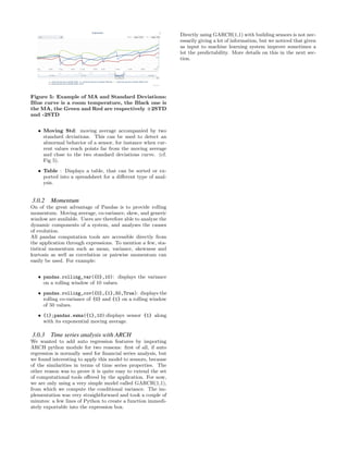
Second, another interesting possibility is to provide rolling
statistic momentum such as moving average, co-variance,
skew, box, or user defined. One is therefore able to ana-
lyze the dynamic components of a system and the causes of
evolution (see below). Last but not least, discrete integra-
tion and derivation, rather important features to describe
thermodynamic models, complete this toolbox. Examples:
• {0}.shift(1);{1}.shift(-1): displays series #0(t+1)
along with series#1(t-1)
• {0}.rolling_window(size,operation) : compute a
rolling operation on a window of given size.
• {0}.diff(): first order derivative with respect to time.
• {0}.diff()/{1}.diff(): first order derivative of texttt{0}
with respect to texttt{1}.
• {0}.cumsum(): integrate value over time.
We will get into more details about rolling momentum in
section 3.
Also, complex lambda function of multiple variables can be
defined , although the syntax is not yet obvious, by using
the special variable namespace pdata, for a full access to the
entire data subset:
pdata.apply(lambda x: x[1] + x[2] if x[0].hour ==2
, axis =1)
will return sum of sensor 0 and 1 for the period from 2 am
to 3 am every day.
2.3.3 Python plugins
A more advanced feature is the ability to develop Python
functions for immediate integration to the application, with
the advantage of being also reachable among users. In the
mean time this is a simple way to encapsulate complex ex-
pressions in order to make one’s work more comprehensible.
Above all, the main advantage is to enlarge the scope of
analysis to a finer level as the plugged in functions can ac-
cess to any combination of row/column data, as well as any
computation library not limited to Pandas. A plugin is cre-
ated by uploading a text file of python code onto the server,
and can be called via a specific namespace from the expres-
sion box, directly applied to variables or as lambda function
from a .apply() type of call. And if the signature allows it,
the plugin can take several sensors as parameters.
2.4 Bulk selection
Bulk selection, another input box, is a way to add into the
sensor stack a set or a list of sensors sharing a pattern of
denomination. This is sometimes easier to do than a man-
ual selection, especially if the number of targeted sensors is
high. That specific kind of request is made of three parts
: a condition of selection, an operation, and a condition on
values. Without going too deep into details of utilization,
we can say this feature is used to highlight all the sensors
from their characteristics of type and location, for which
values have some particularities. For instance a typical re-
quest would be ’give me the list of sensors for every room
of floor X for which the temperature is greater by Y from
the dial temperature’. But the output is sometimes difficult
to visualize on a simple graph so we privileged the Comma
Separated Values format for further analysis with spread-
sheet applications. Unfortunately large requests in terms of
number of sensors involved are huge CPU consumers.
3. COMPUTATIONAL TOOLS
3.0.1 Graphic tools
By default, the application doesn’t require a deep knowledge
of Python, because it allows to create several views on data
without having to define an expression. Different types of
graphs are available to highlight different type of informa-
tion.A graph type is configurable through a menu containing
these choices:
• TimeSeries : regular time series
• XY: merges two data series along time axis and dis-
plays one as function of the other, adding linear re-
gression to the picture.
• Correlation: This is a quick access to correlation
computations, the graphs displayed here are the rolling
correlations of every sensors compared to the first one.
• Histogram: Displays the distribution relative to the
first variable.

5. Figure 5: Example of MA and Standard Deviations:
Blue curve is a room temperature, the Black one is
the MA, the Green and Red are respectively +2STD
and -2STD
• Moving Std: moving average accompanied by two
standard deviations. This can be used to detect an
abnormal behavior of a sensor, for instance when cur-
rent values reach points far from the moving average
and close to the two standard deviations curve. (cf.
Fig 5).
• Table : Displays a table, that can be sorted or ex-
ported into a spreadsheet for a different type of anal-
ysis.
3.0.2 Momentum
On of the great advantage of Pandas is to provide rolling
momentum. Moving average, co-variance, skew, and generic
window are available. Users are therefore able to analyze the
dynamic components of a system, and analyses the causes
of evolution.
All pandas computation tools are accessible directly from
the application through expressions. To mention a few, sta-
tistical momentum such as mean, variance, skewness and
kurtosis as well as correlation or pairwise momentum can
easily be used. For example:
• pandas.rolling_var({0},10): displays the variance
on a rolling window of 10 values.
• pandas.rolling_cov({0},{1},50,True): displays the
rolling co-variance of {0} and {1} on a rolling window
of 50 values.
• {1};pandas.ewma({1},10):displays sensor {1} along
with its exponential moving average.
3.0.3 Time series analysis with ARCH
We wanted to add auto regression features by importing
ARCH python module for two reasons: first of all, if auto
regression is normally used for financial series analysis, but
we found interesting to apply this model to sensors, because
of the similarities in terms of time series properties. The
other reason was to prove it is quite easy to extend the set
of computational tools offered by the application. For now,
we are only using a very simple model called GARCH(1,1),
from which we compute the conditional variance. The im-
plementation was very straightforward and took a couple of
minutes: a few lines of Python to create a function immedi-
ately exportable into the expression box.
Directly using GARCH(1,1) with building sensors is not nec-
essarily giving a lot of information, but we noticed that given
as input to machine learning system improve sometimes a
lot the predictability. More details on this in the next sec-
tion.

6. Figure 6: Machine Learning parameters
4. MACHINE LEARNING, FORECAST AND
MODELING
One interesting thing about this application is that users
have a quick access to some machine learning capabilities,
and rapidly determine a relationship or a dependence be-
tween different types of thermodynamic entities, or also to
validate any physical model, without prior knowledge of
Python programming. Plus those two aspects of the Re-
search process can as well easily shared to other researchers.
Machine learning consists in two phases : training and fore-
casting. The training phase is done with a subset of param-
eters using the sensor selection and the filtering mechanism
describe above, the result of training being persistent. From
there, a forecast or run is performed either with different
parameters, as long as it is consistent with what has been
used for training, and/or different set of values. Results
of training or forecasting are displayed on a specific graph
along with the MSE of the difference between observed and
predicted values. Figure 6 shows an example of training on
a subset made of sensors #0 and #1 for the month of June
2014.
4.1 Input and output
Two types of input are necessary for machine learning : pa-
rameters and values. The parameters set is quite succinct, a
moving average window size, a percentage representing the
training set size and a machine type. Values are defined
through a series of Python-like sub-expressions similar to
what is described in section 3. Similar because the syntax
is the same, but now the order of the sub-expression has a
meaning.
Data input is therefore represented as a list of sub-expressions
separated by commas. But there the first sub-expression will
be the target or forecast value, whereas the following ones
are the observed values. For example, if the expression typed
into the machine learning input box is :
{2};{0}+{3};{1}.diff()
The first sub-expression is {2} meaning sensor #2 is to be
learned; then we have {0}+{3};{1}.diff() which means we
want to fit sensor #2 as a function of a) the sum of sensors
#0 and #3 and b) along with the differential of sensor #1
(with respect to time).
Now this model can be fine tuned by playing on MAW, i.e.
the moving average window size, as well as the machine type,
and the size of the training set.
4.2 Machine Learning models
The machine learning capabilities are still in a trial phase so
for now we limit the set to four regression types of predictors.
• SVM rbf : support vector machine with radial kernel.
• SVM Poly3 : support vector machine with cubic poly-
nomial kernel.
• Logistic Regression: log-linear regression.
• Gaussian:Naive Bayes based on a Gaussian likelihood.
With this sample of different techniques, results so far are
quite promising. All estimators or classifiers come from the
Python sci-kit library, and are based on default parameters
for simplicity. Adding more algorithms from the server code
is pretty straightforward, as the scikit API is very consistent.
4.3 Forecasting and results
To do prediction,we look at the data as time series, and,
similarly to quantitative finance models themselves based on
Markov models, future values are estimated from past data.
Indeed, a rolling window of fixed sized observed at time t de-
termines an estimation of next value, at t+1. To reduce the
number of parameters, past data are reduced to one point, a
moving average. Therefore, a prediction pe0 (t+1) computed
with sub-expression e0 can be seen as a function:
pe0 (t+1) = M(mawe1 (t−s, t), mawe2 (t−s, t), ..., mawei (t−
s), ...)
where maw(t − s, t) is a moving average of size s.
For a given Machine Learning session, three curves are drawn
into the ’Forecast’ widget: The observed value to learn, the
actual output computed by the machine, and the moving
mean square difference.
As said before, the machine learning process has a training
phase and a prediction phase. Once the training done, its
parameters are saved and a prediction can be made from
there with a different set of data, either from different vari-
able or a different time period.
4.4 A case study
The following case study is an attempt to forecast the tem-
perature in a given room during the day. Precisely,as the
time scale consists of 15 minute ticks, the goal is to guess
what will be the room temperature in the next period given
present values of : fan speed, outside temperature, temper-
ature measured at the AHU level (supplied and return), the
actual room temperature, the cooling valve opening in per-
cent. Figure 7 shows the selection stack.
Predicting room temperature can be helpful for energy sav-
ing: the actual AHU system on which that study is based
tends to over correct, and the target temperature is reached
after several oscillations above and below. Forecasting tem-
perature is a way to approximate the thermodynamic model
and directly obtain a target value. The data study is made
over the months of June, July and August, over which tem-
peratures are in the higher range of values. Next figure
illustrate how the data set is restricted to a summer period
of time.
The next step is to define input and output. Here we would
like to know if room temperature can be determined from
the following parameters:

7. Figure 7: Sensor selection for the case study
Figure 8: Filtering for summer months.
• Output is {4} : it is the sensor #4 i.e. temperature in
room 39106.
• First input value is {3} meaning the AHU return tem-
perature.
• Second input value is {t}.hour%4: it is the hour of
observation modulo 4, that represents then a period of
the day roughly mapping the sun course over 24 hours.
• Third input value is {4}
• {1} is sensor #1 so outside temperature.
• {0} corresponds to the AHU fan speed.
• cond_vol{3} for the conditional volatility on a GARCH(1,1)
of the AHU supplied temperature.
• {5}.fillna(0): cooling valve percent where NaN val-
ues are replaced with 0; small problems with raw data
may happen.
• {4}: previous period temperature in target room.
The parameters selection is defined by an expression shown
figure 8, as well as the moving average, and the training set
size; MAW here is set to 1 because the conditional volatility
used as input is already a moving value, and it is comparable
to a variance, so taking its moving average doesn’t make too
much sense. A value of 70 for train size means the training
will use the first 70% of the data set. Finally, a SVM with
radial kernel will be the machine used for this experiment.
After training, machine learning parameters are automati-
cally saved and can be used to predict either the temperature
of a different room, or for a different time period.
5. CONCLUSION
This paper presented a system used for analyzing and build-
ing models from data observed on thousands of sensors. Re-
sults are encouraging as we could explain and approximate
a few thermodynamic behaviors, but yet that system still
lacks of intensive exploitation. It has been devoted by PhD
students within a relatively short period of time and we are
aware that it is still a prototype. Lots of improvements are
necessary, especially in terms of user friendliness and perfor-
mance. But we think it is flexible enough to offers a large
choice of possible utilization and would necessitate from now
on only minor developments. We think still a few concepts
are missing : for instance to store sub-expression results into
variables for later reuse could be very efficient. Same thing
with results of training or forecasting, to generate pipelines
of machine learning computations and then combines mod-
els together. Another point is performance wise some SVM
needs a lot of calculations and could benefit of parallel archi-
tecture.Same remark about bulk selection, which implemen-
tation needs to be optimized if not completely rethought.
Finally, we may now focus on the machine learning part
and modeling, ideally to present another paper based on the
possibility of energy savings using the system.
6. REFERENCES
[1] Highcharts:
http://www.highcharts.com
[2] Pandas: http://pandas.pydata.org
[3] Pandas Time Series
http://pandas.pydata.org/pandas-
docs/stable/timeseries.html
[4] Pandas: computational tools
http://pandas.pydata.org/pandas-
docs/stable/computation.html
[5] Machine Learning in Python
http://scikit-learn.org/stable/