This paper proposes an incremental and adaptive method for 3D reconstruction from a single RGB camera. The key features are: 1) An incremental method for updating the cost volume as new frames are added, without needing to store hundreds of comparison images. This reduces processing time and memory usage. 2) A method for dynamically adapting the minimum and maximum depth limits of the cost volume based on estimated scene depth from a semi-dense reconstruction system. This achieves optimal depth resolution. The algorithm provides dense 3D reconstruction of indoor environments with low computational and memory costs, making it suitable for robotic applications. It is tested on both simulated and real data and shown to outperform previous volumetric reconstruction methods.

1. Incremental and Adaptive Front-End Fusion
Juan M. Falquez, Vincent Spinella-Mamo and Gabe Sibley
Abstract— This paper describes an incremental and adaptive
front-end fusion system capable of providing accurate 3D
models of the world using a single RGB camera. This is
ideal for robotic platforms operating in indoor environments,
where there is a need for high fidelity in the reconstruction
of the world but at a low memory usage and computational
cost. Our algorithm expands on previous volumetric variational
approaches for 3D reconstruction by providing two main key
features. The first is a novel incremental method for updating
the cost volume which removes the need of keeping hundreds
of multi-view comparison images, thus reducing the overall
processing time and memory storage of the system. The second
feature is a method for dynamically adapting the minimum
and maximum depth limits of the cost volume as it adjusts to
changes in scene depth, thus achieving optimum resolution in
the 3D reconstruction.
I. INTRODUCTION
Service robots require spatial information about an en-
vironment in order to interact with it. For example, a robot
moving in a retirement home would need to have an accurate
reconstruction of the scene it is looking at in order to navigate
safely and assist individuals in everyday tasks. Enabling this
on mobile robotics, however, requires fast algorithms with
low memory requirements. Previously, 3D reconstruction of
a scene from multiple images using a monocular camera
has been shown using both local and global methods [12].
In particular, global methods using variational techniques
over a cost volume have shown impressive results for indoor
environments [10]. Despite their ability to reconstruct the
scene with a high level of fidelity, however, these methods are
generally both computationally and memory intensive which
makes them hard to implement in robotic applications.
The objective of this paper is to present a method which
provides good scene reconstruction of indoor environments
while minimizing computational and memory requirements.
Our algorithm provides dense reconstruction of scenes by:
• incrementally adding new frames into a moving cost
volume that is constantly being updated, and,
• adaptively changing the cost volume’s boundaries in
order to adjust to changes in scene depth.
We call our algorithm Incremental and Adaptive Front-End
Fusion (IAFEF), since it is designed to run as the front-end
system for 3D sensing in robotic platforms.
J.M. Falquez (jfalquez@gwu.edu), V. Spinella-Mamo
(vmamo@gwu.edu), and G. Sibley (gsibley@gwu.edu) are
with the Autonomous Robotics and Perception Group, Department of
Computer Science, The George Washington University, Washington, DC
20052, USA
II. RELATED WORK
Perhaps the first work showing how duality methods could
be applied to variational problems is presented in [3]. By
representing the problem as an inequality, the primal-dual
hybrid gradient (PDHG) from linear programming can be
applied to optimizations involving regularization. One of the
first applications of this method to vision problems was the
formulation of the ROF model for denoising [11]. These
duality methods have been applied to more generic computer
vision problems as well [1]. In order to increase the speed
of convergence of these algorithms, adaptive step sizes can
be used [4]. Further work in speeding up primal-dual hybrid
gradients is shown in [7] by creating highly adaptive step
sizes in performing the iterations.
The authors of Dense Tracking and Mapping in Real-
Time (DTAM) [10] have shown that the data term used
in these techniques can be represented volumetrically; that
is, the cost volume stores a sum of photometric errors in
a volumetric representation, where each voxel represents a
sum of photometric errors for a set of comparison images
at a specific depth and pixel coordinate. This volumetric
method, however, introduces a non-convex component in
the global optimization. In general, the primal-dual hybrid
gradient method for global optimization is confined to convex
functions [4]. To overcome this limitation, DTAM proposes
alternating the primal-dual update steps with a finite search
over the cost volume to determine the minimum. The opti-
mization is also augmented by a quadratic relaxation term,
as described in [13]. However, this volumetric approach has
two major limitations.
The first limitation is the discretization of space. Increas-
ing the number of voxels representing depth increases the
precision of the system, i.e. a finer discretization in depth.
This finer level of discretization, however, incurs a higher
computation cost. Every additional level of discretization
requires not only an additional calculation of the photometric
error when constructing the cost volume, but also an addi-
tional step in the search through the cost volume performed
at every iteration.
The second limitation is that the boundaries set on the
cost volume, namely the minimum and maximum depths,
can alter the quality of reconstruction if not properly set. For
example, a far scene with short boundaries will have poor
reconstruction. This is impractical in robotic applications,
since it is known that depth ranges may change greatly as
a robot navigates through the environment. For example, a
robot scanning a desk at close range would require different
depth ranges to one that is navigating down a long corridor.

2. A static boundary on the cost volume results in incorrect
estimates for depth with the changing scene. We show that
it is possible to adaptively expand and contract the volume
by sampling the scene and obtaining a rough distribution of
depth values. By limiting the volume to only visible depth
areas, the system achieves optimum depth resolution.
In addition to the above problems, the reconstruction is
performed over a set of images with an associated set of
relative poses, selecting one image to serve as a reference
image and the others serving as comparison images. To be
useful for mobile robotics, however, the depth needs to be
calculated with respect to the most current frame. The cost
volume must then be constructed based on this reference
image. This means that as the robot moves forward the cost
volume needs to be recomputed at every new frame. This
computation, and storage, becomes prohibitive as the number
of frames fused is increased.
In this paper, we show that an iterative and adaptive
method for forming the cost volume can be used to overcome
the above mentioned problems.
III. METHOD
A. Overview
We follow the same global formulation for our depth
optimization as the one proposed in [10], parameterizing in
inverse depth, namely:
E =
Ω
g(u) ||∇ξ(u)| |ǫ +
1
2θ
(ξ(u) − α(u))2
+λC(u, α(u))dx
(1)
where E is the total cost over the image domain and u is
the pixel coordinate, u : Ω → R2
.
The first term in (1) is a regularizer which enforces second
order smoothness over the inverse depth, ξ. The regularizer
is scaled by a weighting function which serves to reduce
the regularization where there is a large image gradient. The
weighting function g(u) is defined by:
g(u) = e−α|∇Ir(u)|β
2 (2)
Here, α and β are constants selected to vary how much
the image gradient, ∇Ir(u), impacts the weighting of the
regularizer. The regularizer selected is a Huber norm of the
gradient of inverse depth at a pixel coordinate, ||∇ξ(u)| |ǫ.
The last term in (1) is the data term, which is the value
of the cost volume at a specific inverse depth and pixel
coordinate scaled by a factor λ. The cost at a specific pixel
and inverse depth location is the sum of photometric errors
between a reference image and a set of comparison images,
Im.
C (u, ξ(u)) =
1
|Im|
Σm Ir(u) − Im(W(u, ξ(u))) (3)
where W warps the pixel coordinate from the reference
image Ir into each of m comparison images Im, assuming
some estimated inverse depth value ξ(u). W is defined as:
W(u, ξ) = Π KTmr
1
ξ(u)
K−1 u
1
(4)
where Π is a de-homogenization function, K is the camera
matrix and Tmr is the estimated pose between the compari-
son image and the reference image.
Finally, as described in [13], the original cost C and the
regularizer are decoupled via an auxiliary variable, α(u).
This appears as the second term in (1), which shows the
coupling of the estimated inverse depth ξ(u) and the aux-
iliary variable α(u). The variable θ enforces the amount of
coupling, with a smaller θ enforcing stricter coupling. During
a PDHG optimization, θ is reduced at every iteration, thereby
driving the original inverse depth term and auxiliary depth
variables together.
The volumetric representation described above assumes
some discretization of inverse depth, starting from a min-
imum inverse depth ξmin (furthest scene depth) up to a
maximum inverse depth ξmax (closest scene depth). We refer
the reader to the original DTAM paper [10] for more details
on this formulation.
The system alternates between dense tracking and depth
estimation. Dense tracking is performed using a 2.5D Lucas-
Kanade style minimization of photometric errors [2][5] using
the depth maps estimated at each step. Since the system
starts without any depth map, a semi-dense monocular esti-
mation pipeline similar to [6] is used to bootstrap the dense
reconstruction algorithm. After the system is initialized, the
semi-dense algorithm continues to run in the background but
tracking fewer points. These points are then used to adapt
to scene depth, where the minimum and maximum depth
estimates from the semi-dense tracker are used to set the
bounds on the new cost volume. This new volume is then
populated by a linear interpolation of the old volume. The
transformation of the cost volume and rescaling is done in
a single step. After transformation, depth estimation is then
performed by an optimization in accordance with a pixel-
wise gradient ascent/descent in the dual/primal spaces.
B. Incremental
The novel component of our work involves how the
cost volume is computed from frame to frame. To remove
the requirement of keeping multiple images and multiple
transforms between the images, we use a single cost volume
which is incrementally transformed into the most current
reference frame. This assumption is valid as long as the rel-
ative motion from frame to frame is small and is a common
situation encountered in indoor environments, especially for
cameras running at 30 frames per second or more.
Incrementally refining the cost volume from frame to
frame is illustrated as a multistep process, shown in Fig. 1. In
the first step, a new image is captured. In the estimation step,
the newly acquired image and the previous estimate of depth
with its associated intensity image are used to determine the
relative pose of the camera using an RGBD optimization
based on the Efficient Second order Minimization (ESM)
technique as described in [8]. In the transformation step, the
estimated relative pose is used to reinterpret the cost volume
from the perspective of the current frame. As illustrated in
Fig. 2, a new cost volume is placed on top of the old cost

3. Capture Estimate Transform
AddOptimize
Fig. 1. Block diagram of the system. An image is first captured, and
then the relative pose is estimated using whole image alignment. Given
this pose, the cost volumes are transformed and the photometric error with
the current image is added to the volume. Finally, scene depth values are
estimated through the optimization.
(a) (b) (c)
Fig. 2. A top down view of the cost volume at frame N (a) and a visual
depiction of how the cost volume is transformed to a new cost volume
at frame N+1 (b). Darker areas correspond to smaller photometric errors,
indicating a surface. These values are mapped via a trilinear interpolation
onto the new cost volume in (c). Any voxels of the cost volume in frame
N+1 which are not contained in the previous cost volume are marked as
invalid.
volume. The values of the new cost volume are calculated via
a trilinear interpolation. Any locations which do not overlap
are marked as invalid and are not taken into consideration
during the optimization. Once the cost volume is transformed
into the new frame, data from the current image is added.
In computing the traditional cost volume, the sum of all
the photometric errors are stored in an Error Volume (EV)
which is normalized by the total number of images used,
maintained by the Frame Count Volume (FV). In our method,
we separate the photometric errors from the number of
images which have been used to calculate that error and track
them individually. A Normalized Cost Volume (NCV) is then
created by dividing the error by the number of frames that
have reprojected for every pixel and inverse depth location, as
shown in (5). The NCV is calculated on-demand by the depth
estimator and is no longer needed after the optimization ends.
The only volumes that are carried throughout the scene are
the EV and FV.
NCV (u, ξ(u)) =
EV (u, ξ(u))
FV (u, ξ(u))
(5)
Once the EV and FV are transformed to the new frame,
the photometric error of the last image with respect to the
current image, C(u, ξ(u)), is calculated and then added into
the corresponding pixel and inverse depth location in the
cost volume. The frame count for that location is then incre-
mented by one. For any points that do not reproject, there
will be neither an additional cost term nor any addition to
the corresponding frame count volume. In order to overcome
problems associated with occlusions, we down-weight the
previous data exponentially, as shown in the equations below.
EVnew(u, ξ(u)) = C(u, ξ(u)) + ωEVprev(u, ξ(u))
FVnew(u, ξ(u)) = 1.0 + ωFVprev(u, ξ(u))
(6)
Further details regarding the weight parameter ω and its
influence in the cost volume fusion process can be seen in
Section IV.
C. Adaptive
As mentioned before, previous volumetric approaches
use a constant sized cost volume. If improper bounds are
chosen for discretization of the cost volume along inverse
depth, either a significant portion of the information will be
disregarded, or the cost volume will be larger than the scene
to be reconstructed. In either case, this leads to a poor scene
reconstruction. In other words, the bounds of the cost volume
are subject to the following two problems:
1) Over Sizing: A lack of data in the near or far region
of the cost volume indicates that there is no reprojection for
that choice of inverse depth and that the boundaries of the
cost volume should be narrowed. This is done by increasing
ξmin and/or decreasing ξmax.
2) Under Sizing: A large percentage of the data in the
near or far regions of the cost volume indicates that there
is potentially more scene information outside of the bounds
as set and that ξmax should be increased or ξmin decreased,
respectively.
The bounds of the volume, namely ξmin and ξmax, can be
dynamically altered in order to increase the resolution and
accuracy based on the data provided by the semi-dense sys-
tem running in parallel introduced in Section III. The reason
for relying on a secondary system is that it not possible for
any volumetric representation to correctly infer depth values
if the volume bounds are set incorrectly in the first place.
The minimum and maximum depth estimates from the semi-
dense tracker are used to set the scene maximum inverse
depth and minimum inverse depth, respectively, as seen in
Fig. 3.
Once we have calculated the desired range of the cost
volume, ξmin → ξmax, it is possible to use the same
transform function to warp the cost volume to fit the new
space. Any areas of the cost volume that do not fall within
the old volume are marked as invalid.
Fig. 3. Example of how the cost volume is expanded or contracted
depending on estimated inverse depth ranges from the semi-dense tracker.
A trilinear interpolation is used to expand/reduce the cost volume

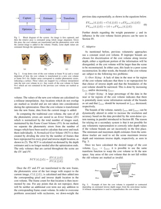
4. IV. RESULTS
We tested our method with both simulated and real data.
For our simulated runs, we use the Tsukuba dataset [9], a
very popular dataset that provides ground truth depth and
has a high variance of depth throughout the sequence. For
our live test, we use a PointGrey Bumblebee camera set in
single image (non-stereo) mode and capture a living room
scene. As an error metric, we show both the average absolute
difference between our estimated depth and the ground truth,
as well as completeness and precision curves.
In order to test how well the reconstruction algorithm
alone performs, any errors associated with pose estimation
and scale ambiguities were removed by using the ground
truth poses. We use the parameters from Table I when
evaluating our proposed method. We also compare with
a simplified version of our algorithm that only performs
incremental volume updates, but does not dynamically adapt
to changes in depth. The incremental only algorithm is
designated by Incremental Front-End Fusion (IFEF) to dif-
ferentiate from the full system that is both incremental and
adaptive, IAFEF.
The final parameter in Table I, ω, controls the contribution
to the incremental update of the cost volume as shown in
(6). This value is directly related to the amount of potential
occlusions in the scene given viewpoint changes. Ideally, the
value should be as high as possible in order to obtain the
maximum contribution from previous estimates into the new
estimate. We plotted the mean error with different values of
ω for a section of the dataset that experiences high viewpoint
changes and obtained Fig. 4.
Although a value of 0.7 seems to give the best performance
for this particular test sequence, for the general case we
selected 0.5, as we believe this to be a conservative value
of ω for any type of scene.
TABLE I
ALGORITHM PARAMETERS
α β ǫ λstart θstart θend ω
100 1.6 10−4 1.0 1.0 10−5 0.5
300 320 340 360 380 400
0
0.5
1
1.5
2
Frame Number
MeanError[meters]
0.1
0.2
0.3
0.4
0.5
0.6
0.7
0.8
0.9
1.0
Fig. 4. Mean Error versus ω as it contributes to the incremental update of
the cost volume. A value of 1.0 would yield the maximum contribution.
A. Timings
We found that the time that it takes to transform the cost
volume is the same as the time to add an image to the cost
volume. This was expected, as the operations are essentially
the same: they both require an evaluation at every pixel and
inverse depth position in the cost volume. In other words,
the time it takes to construct the cost volume for DTAM
is dependent on the number of comparison frames to be
fused, O(M). On the other hand, since there is only a single
comparison image in IFEF, the time to transform and add
the most recent image remains constant, O(1).
Therefore, the speed-up in our implementation is most
noticeable as the number of comparison images is increased.
Regular DTAM uses hundreds of comparison images, but
even with a basic 30 window implementation we can see
that there is a 15x speed-up in the construction of the cost
volume: 30 additions to a cost volume as opposed to the time
it takes to transform the volume and add a single image.
B. Iterative Method
An initial qualitative depth map reconstruction is shown
in Fig. 5. For actual error measurements, we compute
completeness and precision curves comparing a pure in-
cremental approach of IFEF with a 30 windowed DTAM
implementation. This means that our algorithm does not store
any additional frames, but rather transforms the volume and
fuses the current frame at every step. As seen in Fig. 6,
IFEF slightly under-performs compared to a full windowed
version of DTAM, but at a 15x speed-up gain. This is not
unexpected, as the pure incremental IFEF only fuses small
baseline images, whereas DTAM has both small and wide
baselines in the comparison window.
Fig. 5. Images from the Tsukuba sequence with their corresponding depth
maps generated with our approach. The first depth map is of inferior quality,
as it corresponds to the start of the sequence where there is limited data
and little movement.

5. 0 0.02 0.04 0.06 0.08 0.1
0
0.1
0.2
0.3
0.4
Error [meters]
Completeness[%]
IFEF
DTAM30
(a)
0 0.02 0.04 0.06 0.08 0.1
0
0.1
0.2
0.3
0.4
Error [meters]
Precision[%]
IFEF
DTAM30
(b)
Fig. 6. Precision and completeness curves of our algorithm versus a 30
frame windowed version of DTAM. Precision is the percentage of estimates
that are within certain error from the ground truth. Completeness is the
percentage of ground truth measurements that are within certain error of
estimated depth values.
To perform a complete comparison against DTAM, we
use a windowed implementation of IFEF that contains a
mixture of small to large baseline images. Our algorithm
is inherently capable of supporting this hybrid approach, as
the cost volume aggregation can happen whenever frames
drop out of the selected window. This still has the advantage
of a speed-up, as long as the window selected is kept small.
This feature in our algorithm has the extra-benefit of giving
fine control to the user, choosing performance over accuracy
depending on the situation. The result can be seen in Fig.
7, where we tested the above procedure by adjusting the
comparison window and seeing how the error changes with
different window sizes.
Similarly, we tested how DTAM would compare to IFEF
as if it was required to run under the same time constraint.
To do this, we ran DTAM with the number of comparison
selected to yield the equivalent time it takes IFEF to run (two
frames). This comparison is shown in Fig. 8 and illustrates
that our incremental cost volume aggregates more informa-
tion than the two frame window set of DTAM. As can be
seen, incremental front end fusion consistently outperforms
DTAM from frame to frame. This is an indication of the
advantage of using the incremental method, which aggregates
all previous data.
C. Adaptive Window
In order to test our adaptive window, the window size
was changed on every tenth frame using the information
from the semi-dense tracker running in the background. As
can be seen in Fig. 9, the Tsukuba dataset is a particularly
challenging set for a fixed cost volume size implementation,
3 4 5 6
0.3
0.32
0.34
0.36
0.38
0.4
0.42
Number of Comparisons
MeanError[depth]
DTAM
IFEF
Fig. 7. Mean depth error of DTAM versus IFEF with respect to the number
of comparisons performed, where the aggregation of the incremental cost
volume counts as an extra comparison for IFEF.
0 200 400 600 800 1000 1200 1400 1600
0
0.5
1
1.5
2
2.5
Frame Number
MeanError[meters]
IFEF
DTAM2
Fig. 8. Mean depth error for IFEF (red) and DTAM (green) running under
the same time constraint; the equivalent of using two image comparisons.
such as DTAM, given the large variations in scene depth.
Using the estimated depths from the semi-dense features,
we were able to show a marked improvement in the general
depth estimates.
V. CONCLUSIONS & FUTURE WORK
We have shown in this work two improvements in volu-
metric approaches for depth estimation. The first is that it is
possible to incrementally update the cost volume representa-
tion from frame to frame. This incremental approach reduces
the memory and computational time required to reconstruct
a 3D scene from a multi-view stereo and provides depth
estimates at the most current frame. In order to maintain
a constant memory footprint and computation cost during
reconstruction, we show that for small displacements it
is possible to maintain a single cost volume and simply
transform it into the most current frame. This recalculation
allows us to continually estimate depth in the most recent
frame. Results, like those seen in a live sequence in Fig. 10,
show that this approach is comparable, and in most cases,
surpasses traditional volumetric approaches where hundreds
of frames need to be stored and re-calculated at every step.
We have also shown that it is possible to dynamically
change the bounds of the cost volume to produce better
estimates of the scene geometry. This enables mobile robots

6. Fig. 10. Point cloud (a), depth map (b), created from images (c) in a live data sequence using our algorithm. The scene depicts a camera scanning a
bookshelf in a living room environment. High levels of fidelity, as those provided by volumetric approaches to 3D reconstruction, are important for robotic
interaction in indoor environments.
0 200 400 600 800 1000 1200 1400 1600
0
5
10
15
Frame Number
Depth[meters]
Min Depth
Max Depth
(a)
0 100 200 300 400 500 600 700 800
0
0.5
1
1.5
2
2.5
Frame Number
MeanError[meters]
IFEF
IAFEF
(b)
Fig. 9. (a) shows scene minimum and maximum depths per frame in the
Tsukuba dataset. (b) shows how the mean error is improved by using an
adaptive window.
to operate in indoor environments with wide ranges of depth
values, by only selecting the minimum and maximum depth
bounds required to fit the scene in view.
In future work, we plan to implement techniques that
could speed up the depth estimation process itself, which is
the next biggest hurdle now that we have reduced the time
required in building the cost volume. Some work has been
done with Signed Distance Functions (SDFs), which makes
it easy to raycast the depth seen from a particular viewpoint.
We believe it is possible, after the pose is estimated by the
tracker, to use this pose estimate to generate an initial depth
map of the scene given the viewpoint change. This depth map
can therefore be used as an initial value, effectively seeding
the depth optimization by reducing the need to iterate through
all the slices of the cost volume to find the minimum energy.
This has the advantage of allowing us to increase the number
of slices of the cost volume, which is desirable in order to
achieve a finer granularity for the depth estimates, without
incurring the penalty of a higher computation time.
VI. ACKNOWLEDGMENTS
This project was supported by the MITRE Corporation
and Google Inc. All statements of fact, opinion, or analysis
expressed are those of the author and do not reflect the
official positions or views of sponsors.
REFERENCES
[1] J.-F. Aujol. Some first-order algorithms for total variation based image
restoration. Journal of Mathematical Imaging and Vision, 34(3):307–
327, 2009.
[2] S. Baker and I. Matthews. Lucas-kanade 20 years on: A unifying
framework. International journal of computer vision, 56(3):221–255,
2004.
[3] A. Berm´udez and C. Moreno. Duality methods for solving variational
inequalities. Computers & Mathematics with Applications, 7(1):43–58,
1981.
[4] A. Chambolle and T. Pock. A first-order primal-dual algorithm for
convex problems with applications to imaging. Journal of Mathemat-
ical Imaging and Vision, 40(1):120–145, 2011.
[5] A. I. Comport, E. Malis, and P. Rives. Accurate quadrifocal tracking
for robust 3d visual odometry. In Robotics and Automation, 2007
IEEE International Conference on, pages 40–45. IEEE, 2007.
[6] C. Forster, M. Pizzoli, and D. Scaramuzza. Svo: Fast semi-direct
monocular visual odometry. In Proc. IEEE Intl. Conf. on Robotics
and Automation, 2014.
[7] T. Goldstein, E. Esser, and R. Baraniuk. Adaptive primal-dual
hybrid gradient methods for saddle-point problems. arXiv preprint
arXiv:1305.0546, 2013.
[8] S. Klose, P. Heise, and A. Knoll. Efficient Compositional Approaches
for Real-Time Robust Direct Visual Odometry from RGB-D Data. In
IEEE/RSJ International Conference on Intelligent Robots and Systems
(IROS), November 2013.
[9] S. Martull, M. Peris, and K. Fukui. Realistic cg stereo image dataset
with ground truth disparity maps. ICPR workshop TrakMark2012,
111(430):117–118, 2012.
[10] R. A. Newcombe, S. J. Lovegrove, and A. J. Davison. Dtam: Dense
tracking and mapping in real-time. In Computer Vision (ICCV), 2011
IEEE International Conference on, pages 2320–2327. IEEE, 2011.
[11] L. I. Rudin, S. Osher, and E. Fatemi. Nonlinear total variation
based noise removal algorithms. Physica D: Nonlinear Phenomena,
60(1):259–268, 1992.
[12] S. M. Seitz, B. Curless, J. Diebel, D. Scharstein, and R. Szeliski.
A comparison and evaluation of multi-view stereo reconstruction
algorithms. In Computer vision and pattern recognition, 2006 IEEE
Computer Society Conference on, volume 1, pages 519–528. IEEE,
2006.
[13] F. Steinbrucker, T. Pock, and D. Cremers. Large displacement optical
flow computation withoutwarping. In Computer Vision, 2009 IEEE
12th International Conference on, pages 1609–1614. IEEE, 2009.