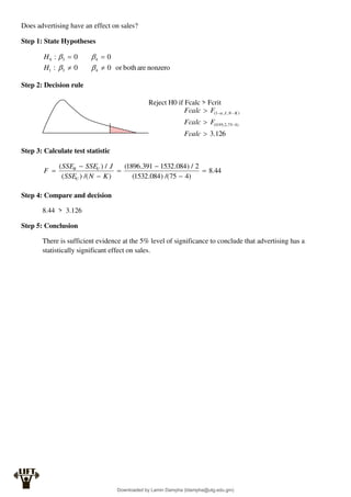
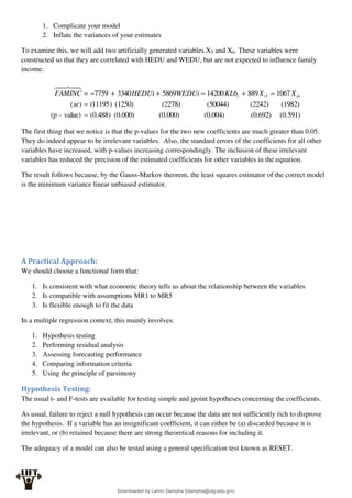
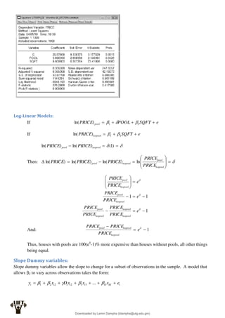
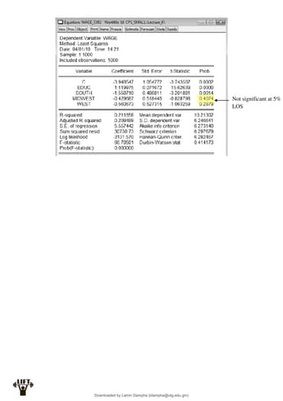
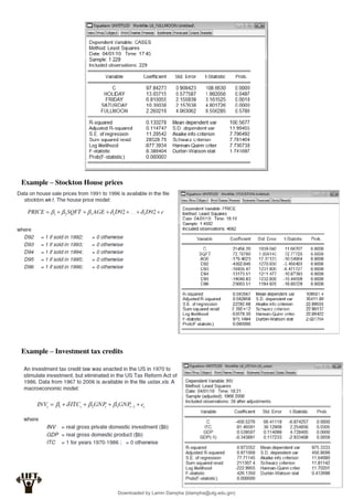
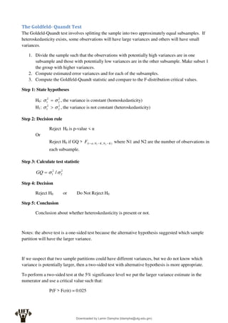
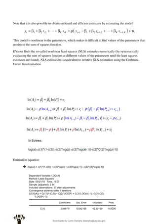
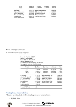
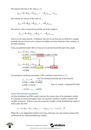
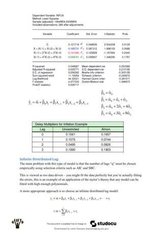
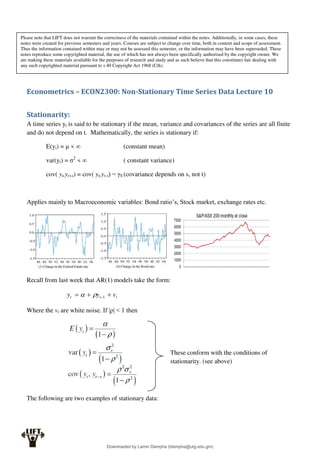
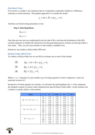
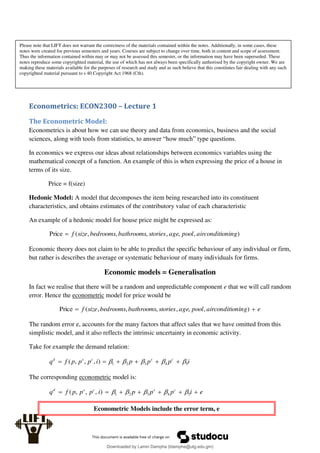
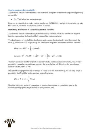
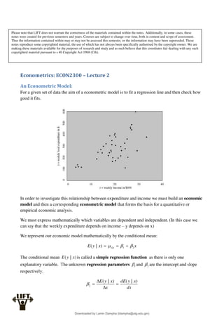
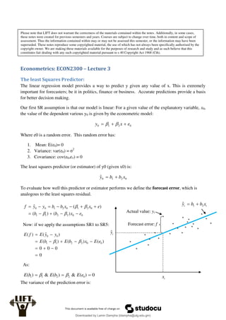
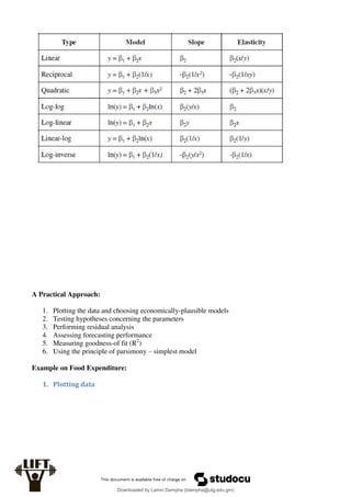
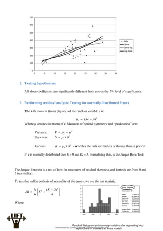
Econometrics uses economic theory and statistical tools to quantify economic relationships and answer questions about economic data. An econometric model includes both a systematic component based on economic theory and an error term that represents unpredictable factors. Most economic data comes from non-experimental sources and is in time-series, cross-sectional, or panel form. The goal of econometrics is statistical inference like estimating parameters, predicting outcomes, and testing hypotheses using sample data. Econometric models incorporate probability distributions, random variables, and concepts like the mean, variance, and normal distribution to analyze economic data statistically.
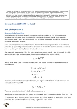
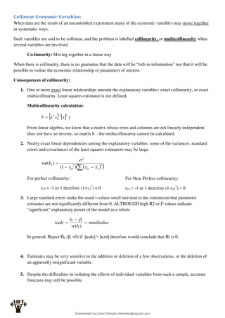
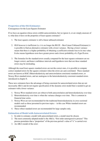
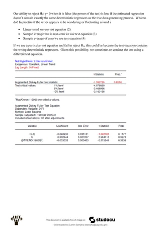
![Laws of Expectation and Variation:
]
[
]
[
]
[
]
[
]
[
]
[
]
[
]
[
]
[
]
[
]
[
]
[
]
[
]
[
0
]
[
]
[
2
2
Y
Var
X
Var
Y
X
Var
Y
E
X
E
Y
X
E
X
Var
a
b
aX
Var
b
X
aE
b
aX
E
X
Var
a
aX
Var
X
aE
aX
E
b
Var
b
b
E
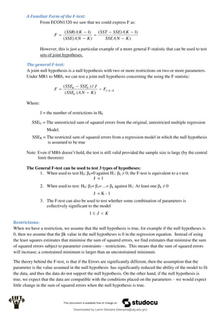
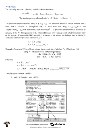
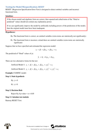
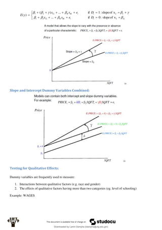
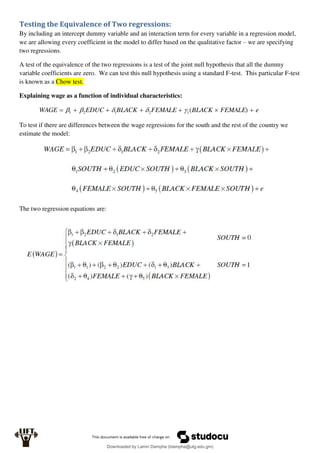
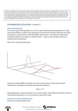
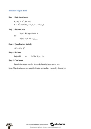
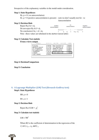
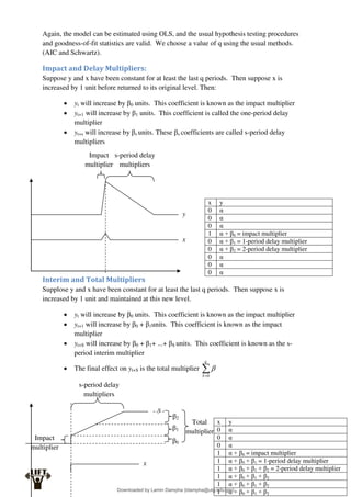
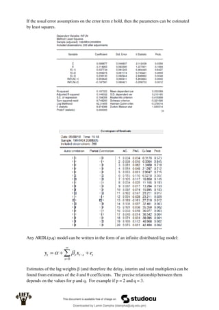
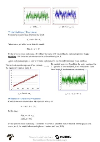
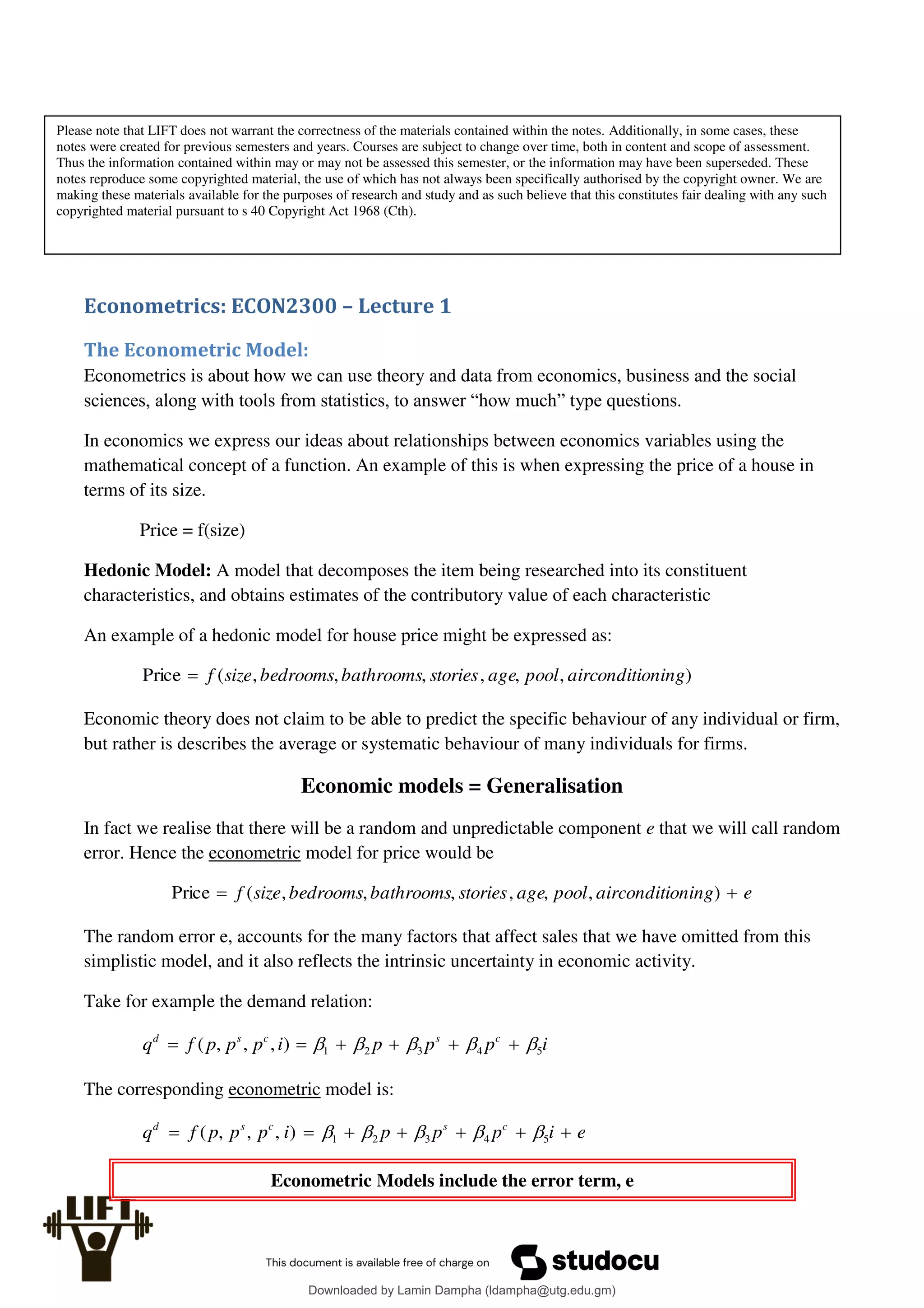
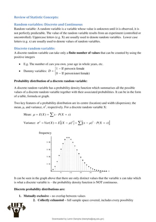
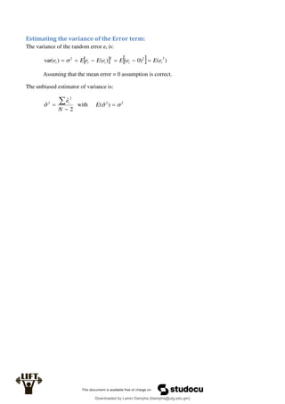
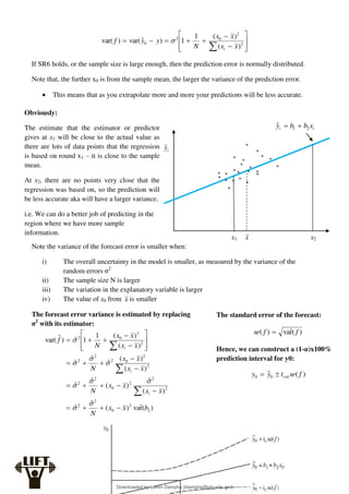
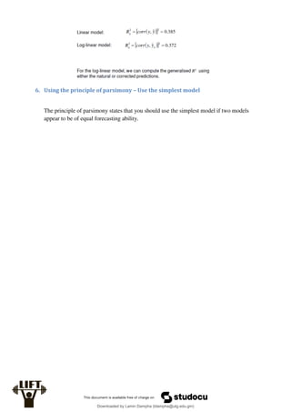
The Error Term:
The error term in a regression model is a random variable. Like other random variables it is
characterised by:
a) A mean (or expected value)
b) A variance
c) A distribution (i.e. probability density function)
We usually assume the random error term of an econometric model to:
a) Have expected value of zero
b) Have a variance which we will call σ2
Where:
a and bare constants
X and Y are random variables
Downloaded by Lamin Dampha (ldampha@utg.edu.gm)
lOMoARcPSD|2941205](https://image.slidesharecdn.com/revision-notes-introductory-econometrics-lecture-1-11-230208195517-de6a877b/85/revision-notes-introductory-econometrics-lecture-1-11-pdf-12-320.jpg)
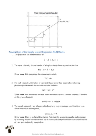
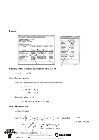
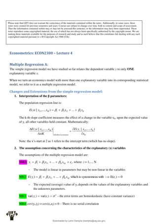
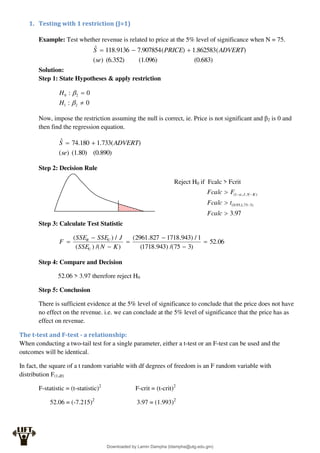
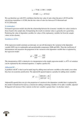
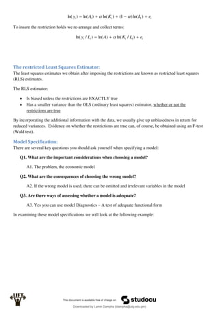
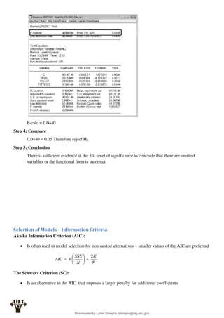
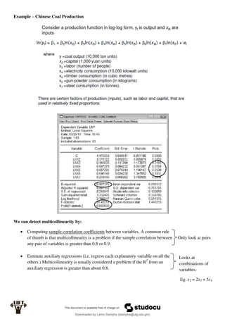
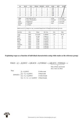
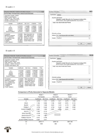
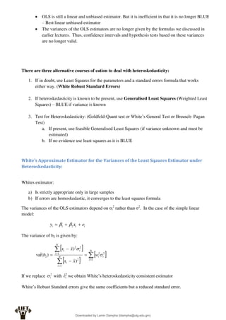
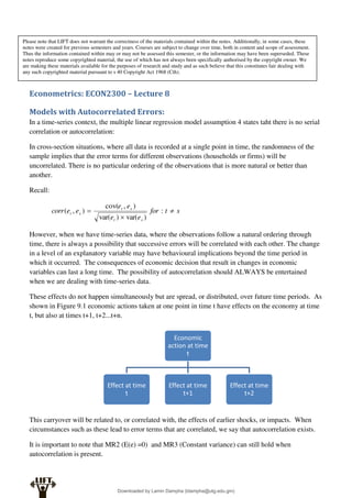
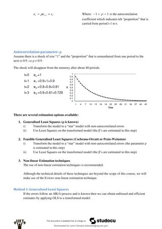
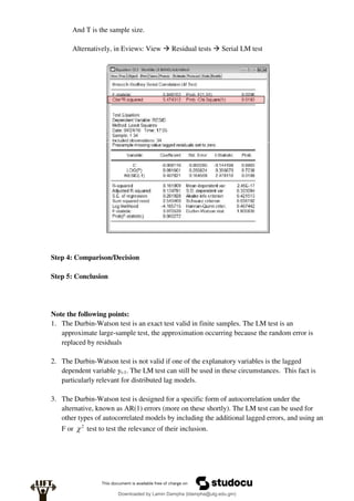
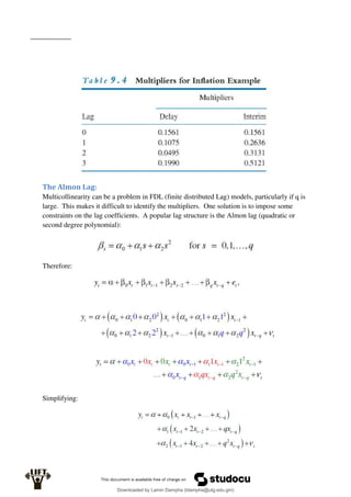
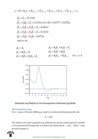
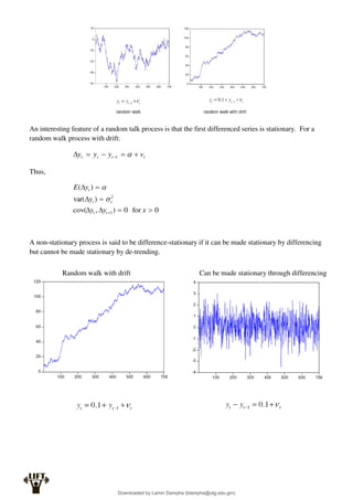
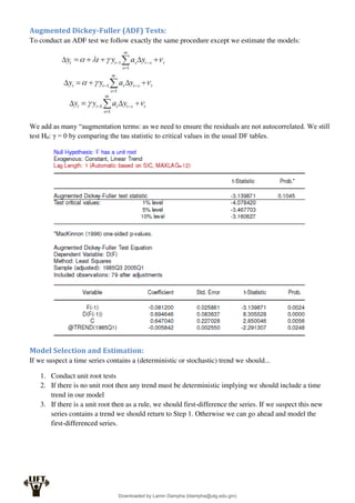
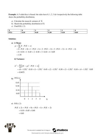
![MR5: The values of each xik are not random and are not exact linear functions of the other
explanatory variables
MR6: (optional) )
,
0
(
~
]
),
...
[(
~ 2
2
2
2
1
N
e
x
x
N
y i
iK
K
i
i
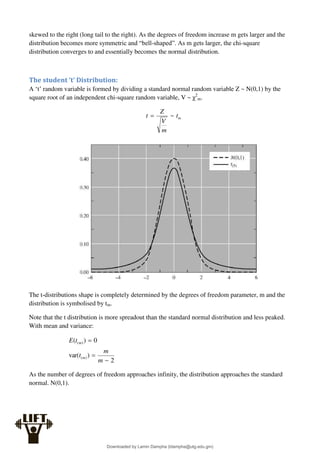
3. The degrees of freedom for the t-distribution
We will go into further detail of this further in the summary.
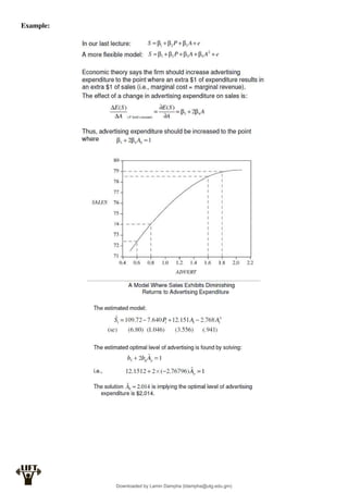
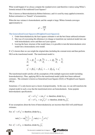
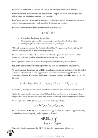
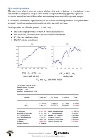
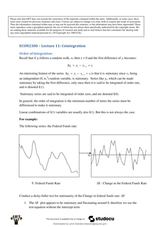
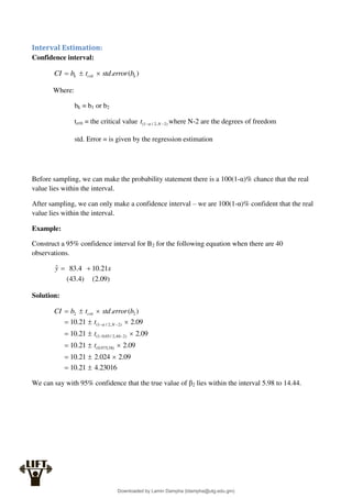
Least Squares Estimation:
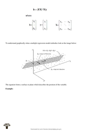
The fitted regression line for the multiple regression model is:
iK
k
i
i x
b
x
b
b
y
...
ˆ 2
2
1
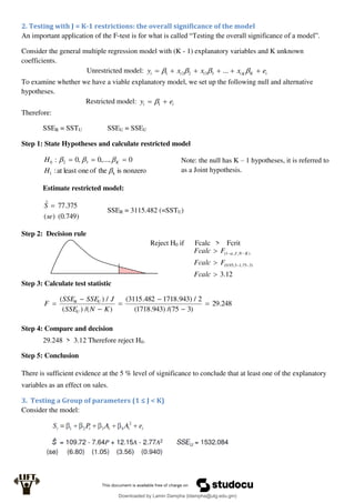
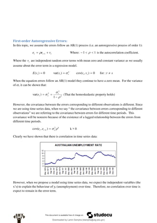
The least squares residual is:
iK
k
i
i
i
i x
b
x
b
b
yi
y
y
e
...
ˆ
ˆ 2
2
1
Similarly to the simple linear regression, the unknown parameters β1,...,βK are obtained by
minimising the residual sum of squares:
N
i
iK
k
i
N
i
i
i
N
i
i x
b
x
b
b
yi
y
y
e
1
2
2
2
1
1
2
1
...
ˆ
ˆ
Solving the first-order conditions for a minimum yields messy expressions for the ordinary least
squares estimators, even when K is small.
For example when K = 3 the OLS method gives:
In practise we use matrix algebra to solve these systems:
Downloaded by Lamin Dampha (ldampha@utg.edu.gm)
lOMoARcPSD|2941205](https://image.slidesharecdn.com/revision-notes-introductory-econometrics-lecture-1-11-230208195517-de6a877b/85/revision-notes-introductory-econometrics-lecture-1-11-pdf-41-320.jpg)