2
Statistics
3
Statistics
The Nature of Statistic
• Definition (Statistics)
Statistics is concerned with
• the collection of data, organization of data,
presentation of data, analysis and
interpretation of data.
Statistics: The science of collecting, describing,
and interpreting data.
4
Introduction to Basic Terms
Population: A collection, or set, of individuals or
objects or events whose properties are to be
analyzed.
Two kinds of populations: finite or infinite.
Sample: A subset of the population.
Example: A college dean is interested in learning about
the average age of faculty. Identify the basic terms in this
situation.
The population is the age of all faculty members at the
college.
A sample is any subset of that population. For example,
we might select 10 faculty members and determine their
age.
The statistic is the “average” age for all faculty in the
sample.
Two Types of Data:
Qualitative Data: data than can be separated
into different categories that are distinguished
by some nonnumeric characteristics.
Note: Arithmetic operations, such as addition
and averaging, are not meaningful for data
resulting from a qualitative variable.
Two Types of Data:
Quantitative Data: consists of numbers
representing counts or measurements.
Note: Arithmetic operations such as addition
and averaging, are meaningful for data
resulting from a quantitative variable.
Qualitative data
• Eye color
• Gender
• color of an apple
• taste of an apple
• smell of an apple
11
Quantitative Data
• Number of TV sets owned by a family
• Number of books in the library
• Time spent on travel to school
• Amount of rainfall
• Weight of an apple
12
Directions: Identify each of the following examples as
attribute (qualitative) or numerical (quantitative) variables.
Write QUALITATIVE or QUANTITATIVE.
1. The residence hall for each student in a statistics class.
2. The amount of gasoline pumped by the next 10 customers
at the Robinsons Mall.
3. The amount of money used for monthly budget.
4. The color of the baseball cap worn by each of 20 students.
5. The length of time to complete a mathematics homework
assignment.
6. The state in which each truck is registered when stopped
and inspected at a weigh station.
Directions: Identify each of the following examples as attribute
(qualitative) or numerical (quantitative) variables. Write QUALITATIVE or
QUANTITATIVE.
7. The temperature in Baler, Aurora at 12:00 pm on any
given day.
8. The make of automobile driven by each faculty member.
9. Whether or not a lantern battery is defective.
10.The weight of a lead pencil.
11.The length of time billed for a long-distance telephone call.
12.The brand of cereal children eat for breakfast.
13. The type of book taken out of the library by an adult.
14. The eye color of Grade 7 Dalton.
15. Time spent on travel to school of Clareans.
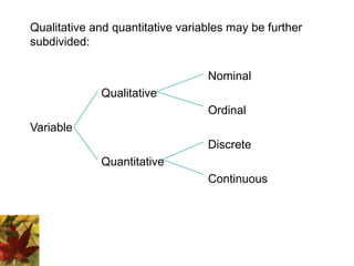
Qualitative and quantitative variables may be further
subdivided:
Nominal
Qualitative
Ordinal
Variable
Discrete
Quantitative
Continuous
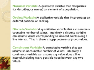
NominalVariable:A qualitative variable that categorizes
(or describes, or names) an element of a population.
OrdinalVariable:A qualitative variable that incorporates an
ordered position, or ranking.
DiscreteVariable:A quantitative variable that can assume a
countable number of values. Intuitively, a discrete variable
can assume values corresponding to isolated points along a
line interval. That is, there is a gap between any two values.
ContinuousVariable:A quantitative variable that can
assume an uncountable number of values. Intuitively, a
continuous variable can assume any value along a line
interval, including every possible value between any two
values.
Statistics deals with numbers
• Need to know nature of numbers collected
– Continuous variables: type of numbers associated
with measuring or weighing; any value in a
continuous interval of measurement.
• Examples:
– Weight of students, height of plants, time to flowering
– Discrete variables: type of numbers that are
counted or categorical
• Examples:
– Numbers of boys, girls, insects, plants
Note:
1. In many cases, a discrete and continuous variable may
be distinguished by determining whether the variables
are related to a count or a measurement.
2. Discrete variables are usually associated with counting.
If the variable cannot be further subdivided, it is a clue
that you are probably dealing with a discrete variable.
3. Continuous variables are usually associated with
measurements. The values of discrete variables are
only limited by your ability to measure them.
Example: Identify each of the following as examples of (1)
nominal, (2) ordinal, (3) discrete, or (4) continuous variables:
1. The length of time until a pain reliever begins to work.
2. The number of chocolate chips in a cookie.
3. The number of colors used in a statistics textbook.
4. The brand of refrigerator in a home.
5. The overall satisfaction rating of a new car.
6. The number of files on a computer’s hard disk.
7. The pH level of the water in a swimming pool.
8. The number of staples in a stapler.
1.3: Measure and Variability
• No matter what the response variable: there
will always be variability in the data.
• One of the primary objectives of statistics:
measuring and characterizing variability.
• Controlling (or reducing) variability in a
manufacturing process: statistical process
control.
Example: A supplier fills cans of soda marked 12 ounces.
How much soda does each can really contain?
• It is very unlikely any one can contains exactly 12 ounces of
soda.
• There is variability in any process.
• Some cans contain a little more than 12 ounces, and some
cans contain a little less.
• On the average, there are 12 ounces in each can.
• The supplier hopes there is little variability in the process,
that most cans contain close to 12 ounces of soda.
1.4: Data Collection
• First problem a statistician faces: how to
obtain the data.
• It is important to obtain good, or
representative, data.
• Inferences are made based on statistics
obtained from the data.
• Inferences can only be as good as the data.
Biased Sampling Method: A sampling method that produces
data which systematically differs from the sampled
population. An unbiased sampling method is one that is not
biased.
Sampling methods that often result in biased samples:
1. Convenience sample: sample selected from elements of a
population that are easily accessible.
2. Volunteer sample: sample collected from those elements
of the population which chose to contribute the needed
information on their own initiative.
Process of data collection:
1. Define the objectives of the survey or experiment.
Example: Estimate the average life of an electronic
component.
2. Define the variable and population of interest.
Example: Length of time for anesthesia to wear off after
surgery.
3. Defining the data-collection and data-measuring schemes.
This includes sampling procedures, sample size, and the
data-measuring device (questionnaire, scale, ruler, etc.).
4. Determine the appropriate descriptive or inferential data-
analysis techniques.
Methods used to collect data:
Experiment: The investigator controls or modifies the
environment and observes the effect on the variable under
study.
Survey: Data are obtained by sampling some of the
population of interest. The investigator does not modify the
environment.
Census: A 100% survey. Every element of the population is
listed. Seldom used: difficult and time-consuming to
compile, and expensive.
Sampling Frame: A list of the elements belonging to the
population from which the sample will be drawn.
Note: It is important that the sampling frame be
representative of the population.
Sample Design: The process of selecting sample elements
from the sampling frame.
Note: There are many different types of sample designs.
Usually they all fit into two categories: judgment samples
and probability samples.
Judgment Samples: Samples that are selected on the basis of
being “typical.”
Items are selected that are representative of the population.
The validity of the results from a judgment sample reflects
the soundness of the collector’s judgment.
Probability Samples: Samples in which the elements to be
selected are drawn on the basis of probability. Each element
in a population has a certain probability of being selected as
part of the sample.
Random Samples: A sample selected in such a way that every
element in the population has a equal probability of being
chosen. Equivalently, all samples of size n have an equal
chance of being selected. Random samples are obtained
either by sampling with replacement from a finite population
or by sampling without replacement from an infinite
population.
Note:
1. Inherent in the concept of randomness: the next result (or occurrence) is
not predictable.
2. Proper procedure for selecting a random sample: use a random number
generator or a table of random numbers.
Example: An employer is interested in the time it takes each
employee to commute to work each morning. A random
sample of 35 employees will be selected and their
commuting time will be recorded.
There are 2712 employees.
Each employee is numbered: 0001, 0002, 0003, etc. up to
2712.
Using four-digit random numbers, a sample is identified:
1315, 0987, 1125, etc.
Systematic Sample: A sample in which every kth item of the
sampling frame is selected, starting from the first element
which is randomly selected from the first k elements.
Note: The systematic technique is easy to execute. However,
it has some inherent dangers when the sampling frame is
repetitive or cyclical in nature. In these situations the results
may not approximate a simple random sample.
Stratified Random Sample: A sample obtained by stratifying
the sampling frame and then selecting a fixed number of
items from each of the strata by means of a simple random
sampling technique.
Proportional Sample (or Quota Sample): A sample obtained
by stratifying the sampling frame and then selecting a
number of items in proportion to the size of the strata (or by
quota) from each strata by means of a simple random
sampling technique.
Cluster Sample: A sample obtained by stratifying the
sampling frame and then selecting some or all of the items
from some of, but not all, the strata.
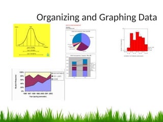
Organizing and Graphing Data
Goal of Graphing?
1. Presentation of Descriptive Statistics
2. Presentation of Evidence
3. Some people understand subject matter
better with visual aids
4. Provide a sense of the underlying data
generating process (scatter-plots)
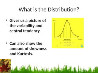
What is the Distribution?
• Gives us a picture of
the variability and
central tendency.
• Can also show the
amount of skewness
and Kurtosis.
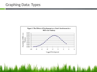
Graphing Data: Types
Creating Frequencies
• We create frequencies by sorting data by
value or category and then summing the
cases that fall into those values.
• How often do certain scores occur? This is a
basic descriptive data question.
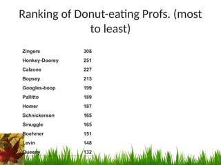
Ranking of Donut-eating Profs. (most
to least)
Zingers 308
Honkey-Doorey 251
Calzone 227
Bopsey 213
Googles-boop 199
Pallitto 189
Homer 187
Schnickerson 165
Smuggle 165
Boehmer 151
Levin 148
Queeny 132
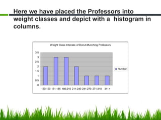
Weight Class Intervals of Donut-Munching Professors
0
0.5
1
1.5
2
2.5
3
3.5
130-150 151-185 186-210 211-240 241-270 271-310 311+
Number
Here we have placed the Professors into
weight classes and depict with a histogram in
columns.
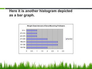
Weight Class Intervals of Donut-Munching Professors
0 0.5 1 1.5 2 2.5 3 3.5
130-150
151-185
186-210
211-240
241-270
271-310
311+
Number
Here it is another histogram depicted
as a bar graph.
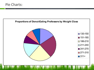
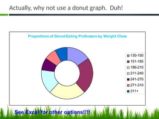
Pie Charts:
Proportions of Donut-Eating Professors by Weight Class
130-150
151-185
186-210
211-240
241-270
271-310
311+
Actually, why not use a donut graph. Duh!
Proportions of Donut-Eating Professors by Weight Class
130-150
151-185
186-210
211-240
241-270
271-310
311+
See Excel for other options!!!!
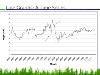
Line Graphs: A Time Series
0
10
20
30
40
50
60
70
80
90
100
Month
Approval
Approval
Economic approval
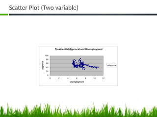
Scatter Plot (Two variable)
Presidential Approval and Unemployment
0
20
40
60
80
100
0 2 4 6 8 10 12
Unemployment
Approval
Approve
1. Terminology
Populations & Samples
• Population: the complete set of individuals, objects
or scores of interest.
– Often too large to sample in its entirety
– It may be real or hypothetical (e.g. the results from an
experiment repeated ad infinitum)
• Sample: A subset of the population.
– A sample may be classified as random (each member has
equal chance of being selected from a population) or
convenience (what’s available).
– Random selection attempts to ensure the sample is
representative of the population.
44
Variables
• Variables are the quantities measured in a
sample.They may be classified as:
– Quantitative i.e. numerical
• Continuous (e.g. pH of a sample, patient cholesterol
levels)
• Discrete (e.g. number of bacteria colonies in a
culture)
– Categorical
• Nominal (e.g. gender, blood group)
• Ordinal (ranked e.g. mild, moderate or severe
illness). Often ordinal variables are re-coded to be
quantitative.
45
Variables
• Variables can be further classified as:
– Dependent/Response. Variable of primary interest (e.g.
blood pressure in an antihypertensive drug trial). Not
controlled by the experimenter.
– Independent/Predictor
• called a Factor when controlled by experimenter. It
is often nominal (e.g. treatment)
• Covariate when not controlled.
• If the value of a variable cannot be predicted in
advance then the variable is referred to as a random
variable
46
Parameters & Statistics
• Parameters: Quantities that describe a
population characteristic. They are usually
unknown and we wish to make statistical
inferences about parameters. Different to
perimeters.
• Descriptive Statistics: Quantities and
techniques used to describe a sample
characteristic or illustrate the sample data
e.g. mean, standard deviation, box-plot
47
2. Frequency Distributions
• An (Empirical) Frequency Distribution or Histogram
for a continuous variable presents the counts of
observations grouped within pre-specified classes or
groups
• A Relative Frequency Distribution presents the
corresponding proportions of observations within the
classes
• A Barchart presents the frequencies for a categorical
variable
48
Example – Serum CK
• Blood samples taken from 36 male volunteers
as part of a study to determine the natural
variation in CK concentration.
• The serum CK concentrations were measured
in (U/I) are as follows:
49