Revenue by DepartmentBlue Lake SportsFirst Quarter Sales by CityDepartmentAtlantaBostonChicagoSan DiegoSt. LouisTotalApparel $ 2,600$ 3,200$ 3,800$ 3,700$ 3,200$ 16,500Baseball $ 3,500$ 1,200$ 1,350$ 2,100$ 2,475$ 10,625Basketball $ 1,800$ 1,800$ 2,250$ 1,400$ 1,750$ 9,000Bike & Skate $ 1,500$ 1,325$ 1,225$ 2,450$ 1,650$ 8,150Exercise $ 2,650$ 2,875$ 3,250$ 3,775$ 2,950$ 15,500Fishing $ 2,350$ 1,035$ 1,250$ 2,750$ 1,450$ 8,835Footwear $ 1,875$ 2,675$ 3,575$ 3,250$ 2,950$ 14,325Game Room $ 1,300$ 1,500$ 1,900$ 1,050$ 1,275$ 7,025Golf $ 4,750$ 875$ 925$ 5,400$ 1,250$ 13,200Hockey $ 850$ 1,875$ 1,950$ 750$ 1,650$ 7,075Hunting $ 2,000$ 1,000$ 650$ 725$ 950$ 5,325Lacrosse$ 1,750$ 1,800$ 1,750$ 1,375$ 1,150$ 7,825Running $ 1,925$ 2,400$ 2,800$ 2,650$ 2,000$ 11,775Winter Sports $ 1,250$ 34,350$ 2,750$ 550$ 1,550$ 40,450Total$ 30,100$ 57,910$ 29,425$ 31,925$ 26,250$ 175,610 Atlanta RevenueBlue Lake SportsJanuary Sales in AtlantaDepartmentWeek 1Week 2Week 3Week 4TotalApparel $ 235$ 325$ 215$ 450$ 1,225Baseball $ 430$ 250$ 180$ 315$ 1,175Basketball $ 85$ 150$ 90$ 200$ 525Bike & Skate $ 200$ 325$ 75$ 175$ 775Exercise $ 150$ 160$ 180$ 170$ 660Fishing $ 75$ 150$ 85$ 200$ 510Footwear $ 500$ 350$ 275$ 330$ 1,455Game Room $ 45$ 75$ 35$ 15$ 170Golf $ 175$ 350$ 580$ 200$ 1,305Hockey $ 85$ 125$ 50$ 35$ 295Hunting $ 125$ 350$ 475$ 450$ 1,400Lacrosse$ 200$ 50$ 65$ 75$ 390Running $ 165$ 235$ 325$ 180$ 905Winter Sports $ 75$ 15$ - 0$ 15$ 105Total$ 2,545$ 2,910$ 2,630$ 2,810$ 10,895 USING MICROSOFT EXCEL 2016 Guided Project 3-3 (Mac 2016) Step 1: Download start file Guided Project 3-3 (Mac 2016 Version) Blue Lake Sports has locations in several major cities and tracks sales by department in each store. For this project, you create a pie chart that shows each store’s share of golf-related sales for the first quarter. You also create a line chart to illustrate week-to-week sales for specific departments in one of the stores and insert sparklines in the data. Skills Covered in This Project • Create, size, and position a pie chart object. • Create a line chart sheet. • Apply a chart style. • Apply a chart layout. • Change the chart type. • Insert and format sparklines in a worksheet. • Add and format chart elements. 1. Open the BlueLakeSports-03 start file. If the workbook opens in Protected View, click the Enable Editing button so you can modify it. The file will be renamed automatically to include your name. Change the project file name if directed to do so by your instructor, and save it. NOTE: If group titles are not visible on the Ribbon, click the Word menu and select Preferences to open ...

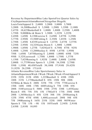
1. Revenue by DepartmentBlue Lake SportsFirst Quarter Sales by
CityDepartmentAtlantaBostonChicagoSan DiegoSt.
LouisTotalApparel $ 2,600$ 3,200$ 3,800$ 3,700$
3,200$ 16,500Baseball $ 3,500$ 1,200$ 1,350$ 2,100$
2,475$ 10,625Basketball $ 1,800$ 1,800$ 2,250$ 1,400$
1,750$ 9,000Bike & Skate $ 1,500$ 1,325$ 1,225$
2,450$ 1,650$ 8,150Exercise $ 2,650$ 2,875$ 3,250$
3,775$ 2,950$ 15,500Fishing $ 2,350$ 1,035$ 1,250$
2,750$ 1,450$ 8,835Footwear $ 1,875$ 2,675$ 3,575$
3,250$ 2,950$ 14,325Game Room $ 1,300$ 1,500$
1,900$ 1,050$ 1,275$ 7,025Golf $ 4,750$ 875$ 925$
5,400$ 1,250$ 13,200Hockey $ 850$ 1,875$ 1,950$
750$ 1,650$ 7,075Hunting $ 2,000$ 1,000$ 650$ 725$
950$ 5,325Lacrosse$ 1,750$ 1,800$ 1,750$ 1,375$
1,150$ 7,825Running $ 1,925$ 2,400$ 2,800$ 2,650$
2,000$ 11,775Winter Sports $ 1,250$ 34,350$ 2,750$
550$ 1,550$ 40,450Total$ 30,100$ 57,910$ 29,425$
31,925$ 26,250$ 175,610
Atlanta RevenueBlue Lake SportsJanuary Sales in
AtlantaDepartmentWeek 1Week 2Week 3Week 4TotalApparel $
235$ 325$ 215$ 450$ 1,225Baseball $ 430$ 250$
180$ 315$ 1,175Basketball $ 85$ 150$ 90$ 200$
525Bike & Skate $ 200$ 325$ 75$ 175$ 775Exercise $
150$ 160$ 180$ 170$ 660Fishing $ 75$ 150$ 85$
200$ 510Footwear $ 500$ 350$ 275$ 330$ 1,455Game
Room $ 45$ 75$ 35$ 15$ 170Golf $ 175$ 350$ 580$
200$ 1,305Hockey $ 85$ 125$ 50$ 35$ 295Hunting $
125$ 350$ 475$ 450$ 1,400Lacrosse$ 200$ 50$ 65$
75$ 390Running $ 165$ 235$ 325$ 180$ 905Winter
Sports $ 75$ 15$ - 0$ 15$ 105Total$ 2,545$ 2,910$
2,630$ 2,810$ 10,895

2. USING MICROSOFT EXCEL 2016 Guided Project 3-3 (Mac
2016)
Step 1:
Download
start file
Guided Project 3-3 (Mac 2016 Version)
Blue Lake Sports has locations in several major cities and
tracks sales by department in each store. For this project, you
create a pie chart that shows each store’s share of golf-related
sales for the first quarter. You also create a line chart to
illustrate week-to-week sales for specific departments in one of

3. the stores and insert sparklines in the data.
Skills Covered in This Project
• Create, size, and position a pie chart object. • Create a line
chart sheet.
• Apply a chart style. • Apply a chart layout.
• Change the chart type. • Insert and format sparklines in a
worksheet. • Add and format chart elements.
1. Open the BlueLakeSports-03 start file. If the workbook opens
in Protected View, click the Enable
Editing button so you can modify it. The file will be renamed
automatically to include your name.
Change the project file name if directed to do so by your
instructor, and save it.
NOTE: If group titles are not visible on the Ribbon, click the
Word menu and select Preferences to
open the Word Preferences dialog box. Click the View button
and check the Show group titles
check box under Ribbon. Close the Word Preferences dialog
box.
2. Create a pie chart object.
a. Select the Revenue by Department sheet, select cells A4:F4,
press command, and select
cells A13:F13.
b. Click the Recommended Charts button [Insert tab, Charts
group].
c. Choose Pie.
3. Apply a chart style.
a. Select the chart object.
b. Click the More button [Chart Design tab, Chart Styles group].

4. c. Select Style 12.
4. Size and position a chart object.
a. Point to the chart object border to display the move pointer.
b. Drag the chart object so its top left corner is at cell A21.
c. Point to the bottom right selection handle to display the
resize arrow.
d. Drag the pointer to cell G35.
5. Change the chart type.
a. Select the pie chart object and click the Change Chart Type
button [Chart Design tab,
Type group].
b. In the drop-down list point to Pie.
c. Choose 3-D Pie.
6. Format pie chart elements.
a. Double-click the pie to open its Format Data Series task pane.
b. Click the Atlanta slice to update the pane to the Format Data
Point task pane. (Rest the
pointer on a slice to see its identifying ScreenTip.)
c. Click the Series Options button in the Format Data Point task
pane.
d. Set the pie explosion percentage at 10%.
e. Close the task pane.
f. Click the chart object border to deselect the Atlanta slice.
Excel 2016 Chapter 3 Creating and Editing Charts Last
Updated: 11/30/17 Page 1

5. 10
11
l2
l3
14
lS
16
l7

6. 18
19
20
21
22
23
24
25
26
27
28
29
30
31
32
" 34
35
36
"
A C

7. £xerci se -s- 2~Gso -s- 2:s1s -s-3:2so
Fishi ng s 2,350 s 1,035 s 1,250
Foot wea r s 1,875 s 2,675 s 3,575
Gc1 me Room 1,300 1,500 1,900
Golf 4,750 875 925
Hockey 850 1,875 1,950
Hu nting 2,000 1,000 650
LacrGSse 1,750 1.800 1.750
Runn ing 1,925 2,400 2,800
Winter Sports 1,250 34, 350 2,750
Total s 30, 100 57,9 10 29,425
' Golf
F G
-s- 3:11s s- 2:9so -s-is;soo:rj
s 2,750 S 1.450 S 8,835
s 3,250 S 2,950 S 14,325
1,050 1.27S 7,025
5,400 1,250 13, 2 00
750 1.650 7,075
725 950 5,325
1,375 1.150 7,825
2,650 2,000 ll,775
550 1.550 40,450
31,925 26, 250 175,610

8. Format Data Labels
@[email protected]•fuUlj,tp Text Options
Ii 1 1
T Label Op ti ons
Label Contains
0 Series name
0 Category name
O va1ue
II Percentage
II Show leader lines
n Legend key
Separator
Reset Label Text
, (c omma)
Revenue by Departmenl Atlanta Revenue +
Label Position
n center
chart Ti tle
..,,
~

9. ""'
,.
=
I
~ -!
""'
""'
"'"
""
Wodl .. ,.., ..... , .....
S>I! ,.,. S,15 '"' $1., - ,.., ... mo ...
3-67 Data tab le added by Quick Layout
USING MICROSOFT EXCEL 2016 Guided Project 3-3 (Mac
2016)
7. Add and format chart
elements in a pie chart.
a. Click the Add Chart
Elements button
[Chart Design tab,
Chart Layouts group].
b. Point to Data Labels.
c. Choose More Data
Label Options...
d. Click the Label

10. Options button In the
Format Data Labels
pane.
e. Click Label Options to
expand the group.
f. Select the Percentage
box.
g. Deselect the Value box (Figure 3-66).
h. Press command+B to apply bold.
i. Change the font size to 12 pt [Home tab, Font group].
j. Click the chart object border to select it.
k. Click the Shape Outline button [Chart Format tab, Shape
Styles group] and choose Purple,
Accent 4, Darker 50%.
l. Click the Shape Outline button and choose Weight and 1 pt.
m. Click a worksheet cell.
8. Create a line chart sheet.
a. Select the Atlanta Revenue
sheet tab.
b. Select cells A4:E7.
c. Click the Recommended
Charts button [Insert tab,
Charts group].
d. Select Line.
e. Click the Move Chart button
[Chart Design tab, Location

11. group].
f. Click the New sheet button.
g. Type Promo Depts and
click OK.
9. Apply a chart layout.
a. Click the Quick Layout
button [Chart Design tab,
Chart Layouts group].
b. Select Layout 5 to add a data table to the chart sheet (Figure
3-67).
3-66 Format Data Labels task pane
Excel 2016 Chapter 3 Creating and Editing Charts Last
Updated: 11/30/17 Page 2

12. ..
- --- 111•
.. -
~
-· -
Format Dat a Series ...... ,.,.... ~
0
,_
•· Bwl-n
...
fjdar11 a 1 bl':rtU'IIRi
P, Hnn fll
•.-.ut cirru lic:
l
3-68 Marker options for the data series
Home Insert Page Layout Fomiulas Data Review
Se ries · Baseball ~ c:is ..
Chart Area
Chart Title
Data Table Sh>p• St,'os

13. Horizontal (Category) Axis I Reven ue'1$A$ 6,'At lant a Revenu
Plot Area
Vertical (Value) Axis s
Vertical (Value) Axis Major Gridlines
Vertical (Value) Axis Title
Series • Apparel •
,/ Series • Baseball '
Series • Basketball •
400
350
300
250
200
150
100
50
USING MICROSOFT EXCEL 2016 Guided Project 3-3 (Mac
2016)
10. Change the chart type.
a. Click the Change Chart Type button [Chart Design tab, Type
group].
b. Point to Line and choose Line with Markers.
c. The chart now displays point markers.

14. 11. Edit chart elements in a line chart.
a. Click the chart title placeholder.
b. Type Special Promotion Departments in the formula bar and
press Enter.
c. Click the vertical axis title placeholder.
d. Type Dollar Sales in the formula bar and
press Enter.
e. Click the Chart Elements drop-down arrow [Chart Format tab,
Current Selection group].
f. Choose Series “Apparel” to select the line in
the chart.
g. Click the Format Pane button [Chart Format
tab, Format group].
h. Click the Fill & Line button in the Format Data
Series task pane.
i. Click Marker and then click Marker Options to
expand the group (Figure 3-68).
j. Choose Built-in and select 10 pt.
k. Choose Series “Baseball” to select the line in
the chart. (Figure 3-69).
l. Apply the same marker changes for the
baseball series.
m. Select the basketball series and make the
same marker changes.
n. Close the task pane and click outside the
chart.

15. 3-69 Data Series selected
Excel 2016 Chapter 3 Creating and Editing Charts Last
Updated: 11/30/17 Page 3
USING MICROSOFT EXCEL 2016 Guided Project 3-3 (Mac
2016)
Step 2:
Upload &
Save
Step 3:
Grade my
Project

16. 12. Insert sparklines in the worksheet.
a. Click the Atlanta Revenue tab.
b. Right-click the column F heading and choose Insert.
c. Select cells B5:E18 as the data range.
d. Click the Sparklines button and select Line [Insert tab,
Sparklines group].
e. Select cells F5:F18 in the Select where to place sparklines:
box.
f. Click OK.
13. Format sparklines in worksheet.
a. Click the Format button [Home tab, Cells group] and change
the Row Height to 24. NOTE:
Some versions of Macintosh Excel 2016 use inches for row
height and column width. When
viewing the row height, if double quotes appear when
displaying the value, enter 0.33”
instead of 24.
b. Click the Format button [Home tab, Cells group] and set the
Column Width to 35. NOTE:
Some versions of Macintosh Excel 2016 use inches for row
height and column width. When
viewing the column width, if double quotes appear when
displaying the value, enter 2.97”
instead of 35.
c. Select the Markers box in the Show group in the Sparkline
Design tab.
d. Click the Sparkline Color button [Sparkline Design tab, Style
group].
e. Choose Black, Text 1 for the line color.
f. Click cell A1.

17. 14. Change the page orientation to landscape.
15. Save and close the workbook (Figure 3-70).
16. Upload and save your project file.
17. Submit project for grading.
Excel 2016 Chapter 3 Creating and Editing Charts Last
Updated: 11/30/17 Page 4
- -·· "" -. .. ..
Dc:parilmen4;
J..pp:a,-e l
B&..e b;,l l
Baske tb ~II
etke & sir.rot
Ei<:~ rtt;e
F~ lrti:
Fo11~ar
Gz:rnc li! ocrn
Gdf
Hockev

18. HY'l t in!
L;ii:rosse
!'il,l'l t-lng
Wlnt t r Sp ijrt:;
A1la1111i
s 2,li01l s:
$ 3,5011 s:
s ll,il01l s.
~ 1,;;on s.
$ 2.liSll s.
s ;uStl S,
S, 1.07-S s:
S, :l,!1 011 s:
s 4,,7511 s:
s 85!1 s.
$ 2,00!1 S:
~ USD s.
s :UlS s;
s l;.:lSO S,
Tobil S, !IQlOD s:
Blue Lake Sports
Fi rst Qua--e,i $ales b l' Clty
l~nlt"1 Oil~ Sii, rn l!Jle'R"D 'St. lol!ll J I Tot.i,I
S; 200 $ S, [email protected] O $ S, .'[email protected] $ s. 200
Is 16.,&1 0
uoo s 1..~so s 2, 101) $ 2,4 75 11$ 10,625
1,.8 00 s 2,. 250 s 1., ,100 $ 1,,50 IS 9, 000
l..325 :. l 22 5 :; 2 qso $ 1.660 II s 8 15 0
2.87.5 :. ~ 250 s 5,775 $ [email protected] 11$ ILS, 500

19. l,.IHIS $ U5Qi $ ;;f7SQ $ J.,q50 Is S,8;1$
2_,,fjj'§ s 31, !i,7- S $ ] fill) $ 2,!!§0 11,: 14 ,3.2!!
1,'SOD s: 1, 900 s 1) !.SO s 1,:?75 IS 7, 02S
8 75 s 925 s 5, 40 0 $ 1. 25 0 II S 13,XI O
1,.8 7.5, s 1,950 s ,so _j 1 650 ll_j 7 075
1.0001 s 650 s .'25 $ 950 Is 5, S25
l.80D :. 1. 150 :', 1,~s $ u s @ 11 s 7,8"2 5
l ~illO $ :Uli!O $ :!'~I) $ 2.000 Is U, ,'11$
:al ~.~5D :. l.~5 Qi $ 55 0 $ J.,550 Is ~0,450
'!l 7,91JO s 1 91. 42!. $ 3192!, s 2G.~ Is !?!3,dlO
Go lf
an Dei::o 1wr5t . Lou o
i!li!Jc l..,k c Spo rt ~
~WlinA:llil't"..1
""-'"-' ' Ii,"- • ,_. , ..... , M...ii:111 -· ...... m : ~~ ' l:l ! ' .,. ------
--------I Wd:fl ... ' ,.,, I ... ' :u l --------, i.w,, .. .. . ,., . " . Z I ~--
- ---
lii r ~~ a. llllir ' .... , .... ,, . ,,, --------- -, ..
'
.,,, I ... ' ,,, ~_,..... , _ _, n • ,., ' .. ' ZI ~----- ---..... a.!! .. ' ..,. .
1"' ' '" ' . .. ------, ..... l->.:-illl ,, ' ... I ,. j ,. ~----.... :. r, • ,., ' ...
. ZI ~~ ----i-,- 1" ' .. . ,,., ' .. ' --,._n .,.
'
,., I !!;.'Ii I ..,, ·------
1..-.... .... ... . .. . .. ' " -....
.., .,.,

20. ~ .1.......l!:: "" ~- -- -._ "MU.i i' :X.'ll, n ' .. ' I .. --.... ""' .... ..
II: :11 11 . :-ua ' '"'' ' Ull
,.,.
1~ 1.13
• u H ,,.
1, ,.,.
t -
'"
1, " "' t ,,.
, ..
1, "" It ·--,, -. ... .....
3 -70 Excel 3-3 comple t,ed worksheet am:11 ch arts
USING MICROSOFT EXCEL 2016 Guided Project 3-3 (Mac
2016)
Excel 2016 Chapter 3 Creating and Editing Charts Last
Updated: 11/30/17 Page 5
Guided Project 3-3 (Mac 2016 Version)Skills Covered in This
Project