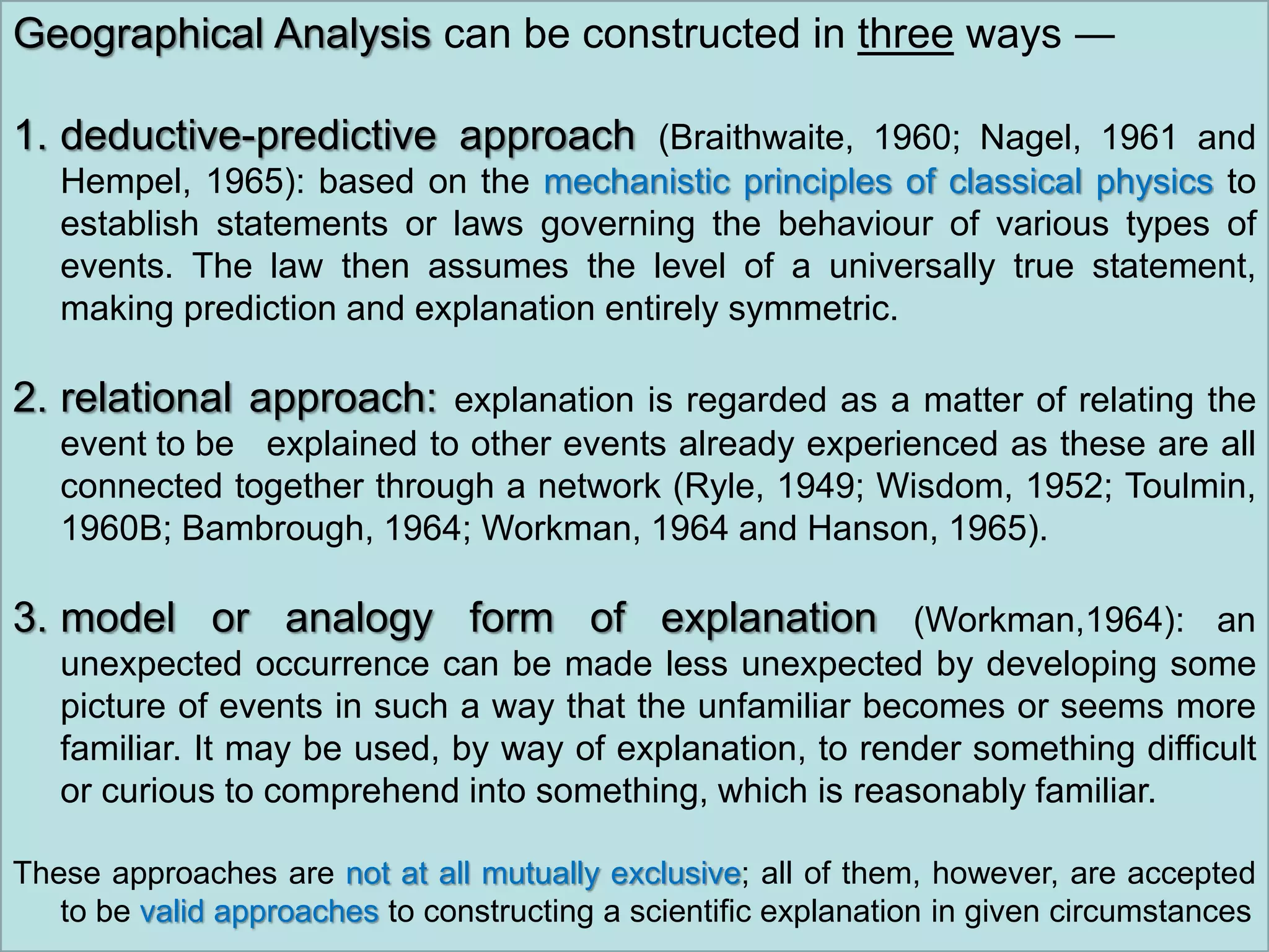
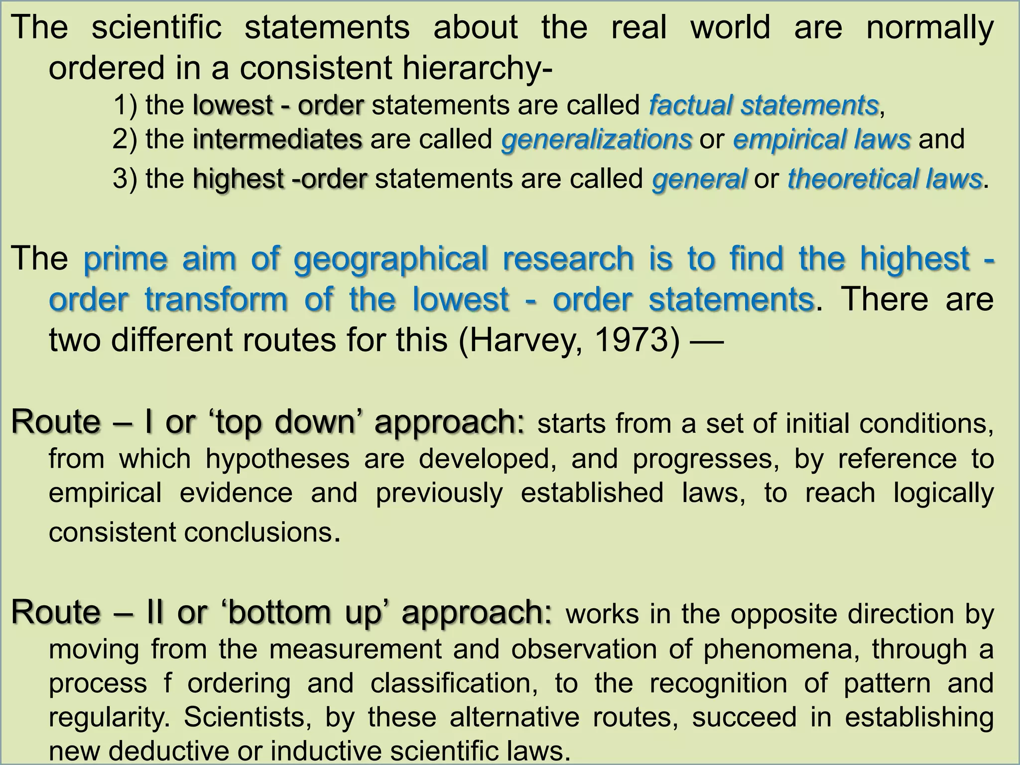
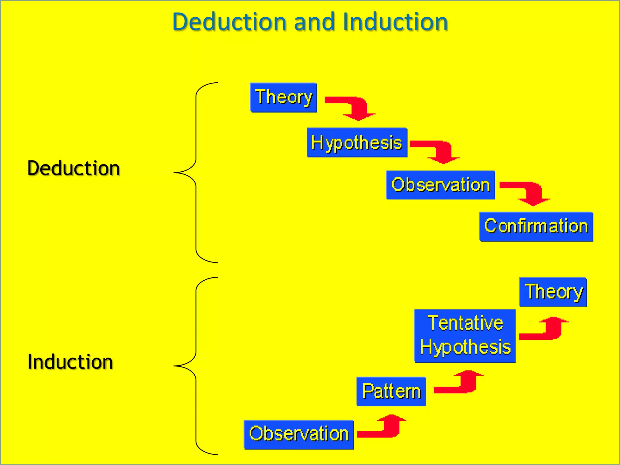
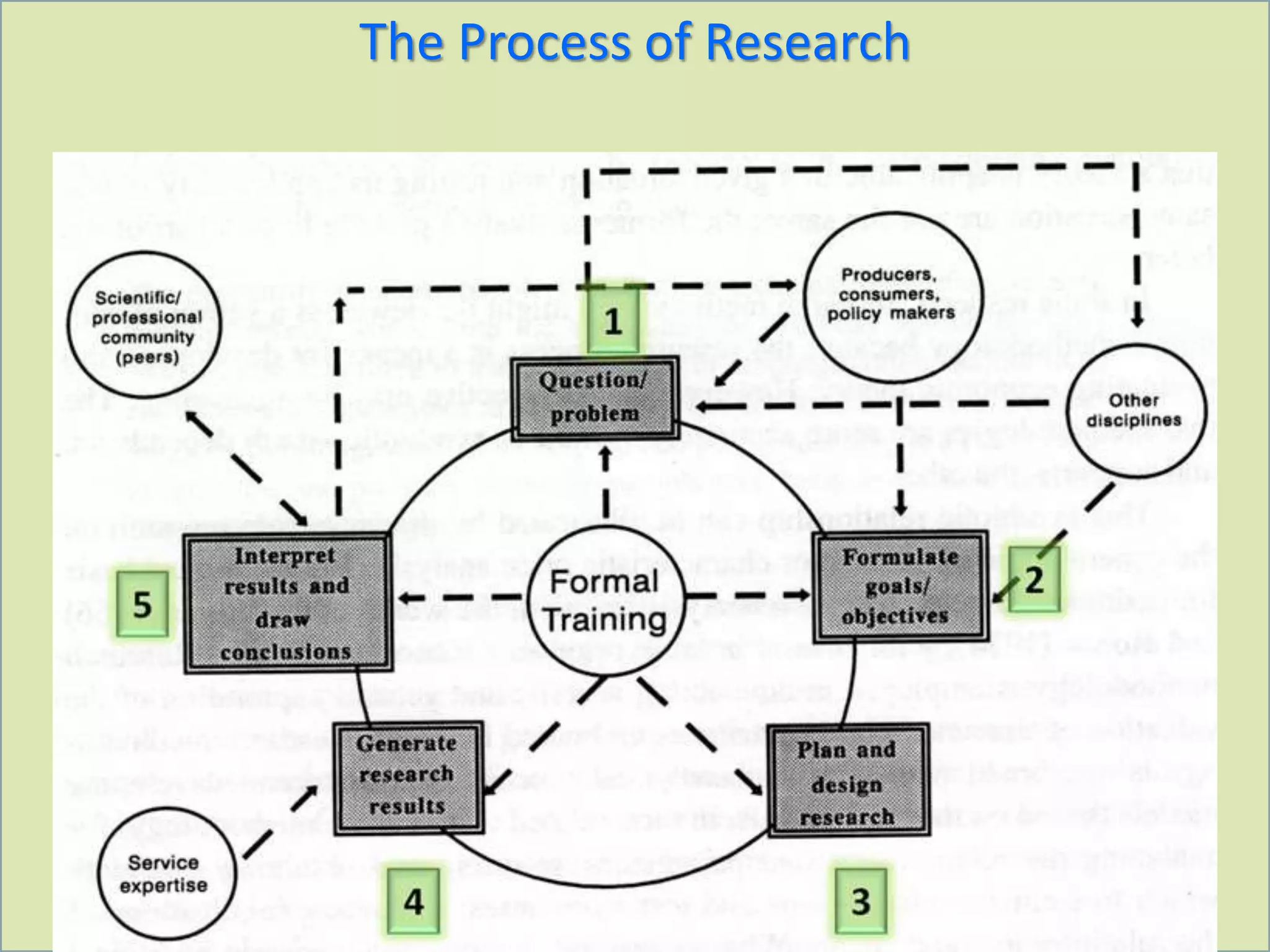
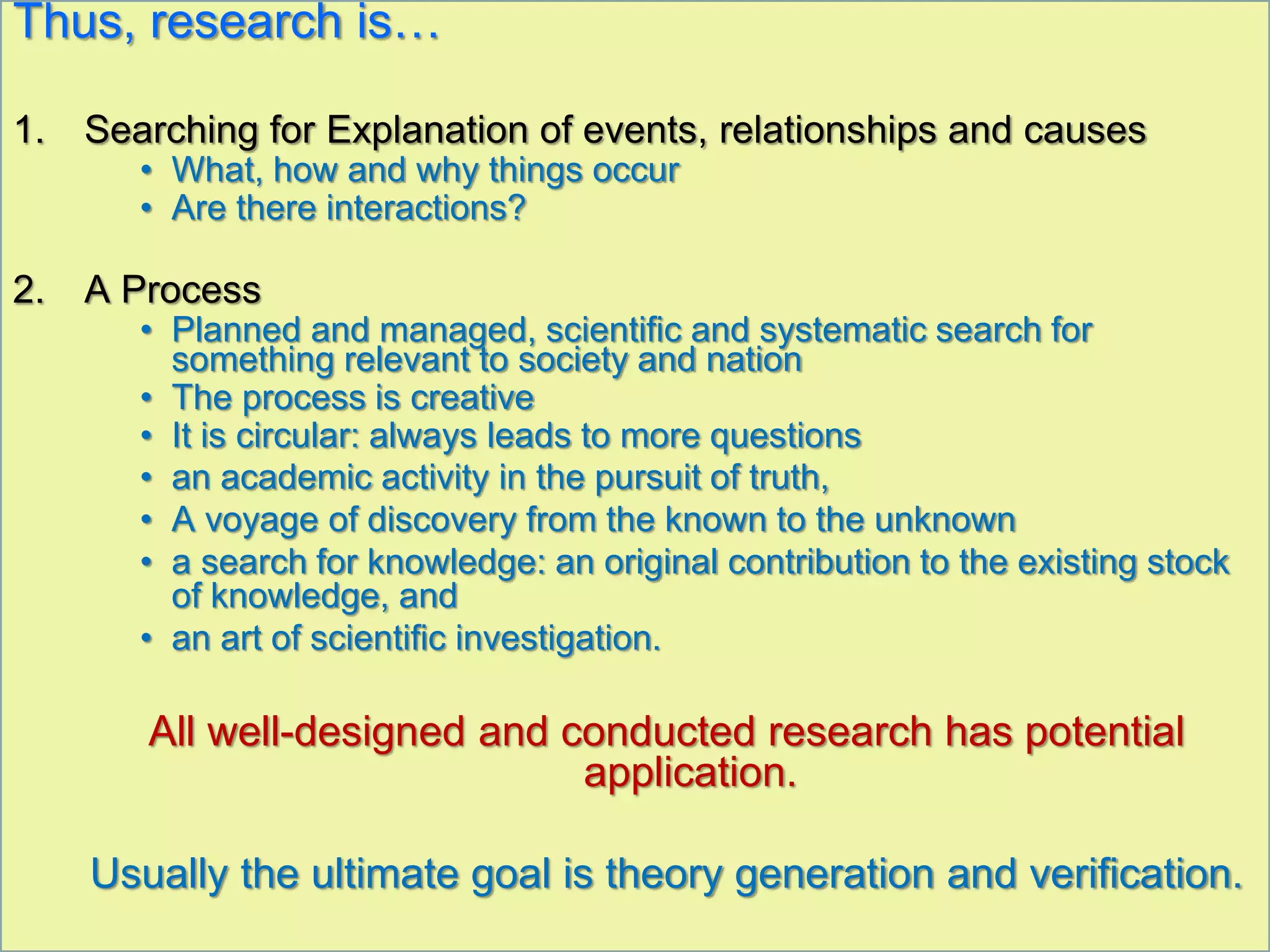
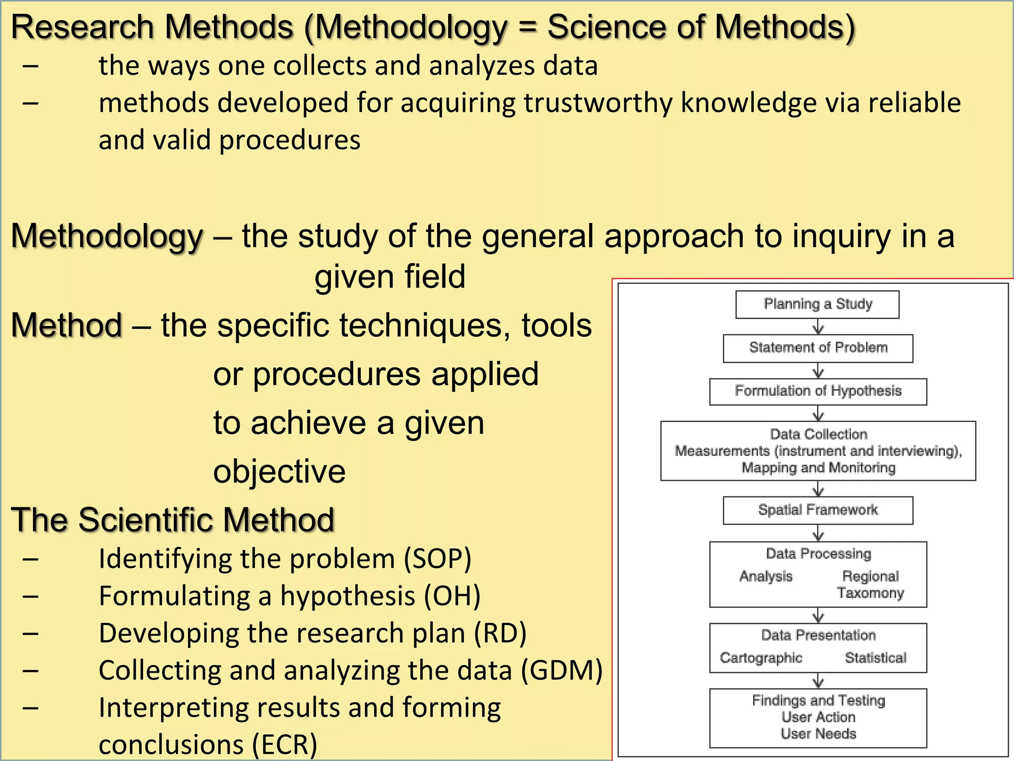
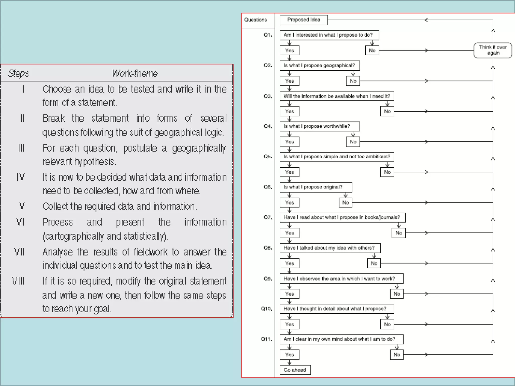
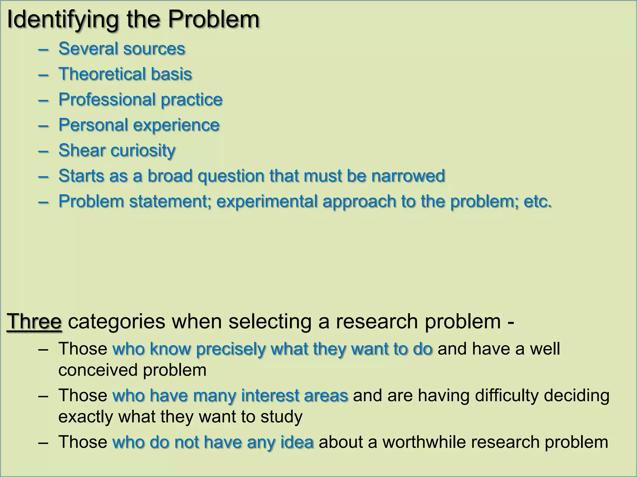
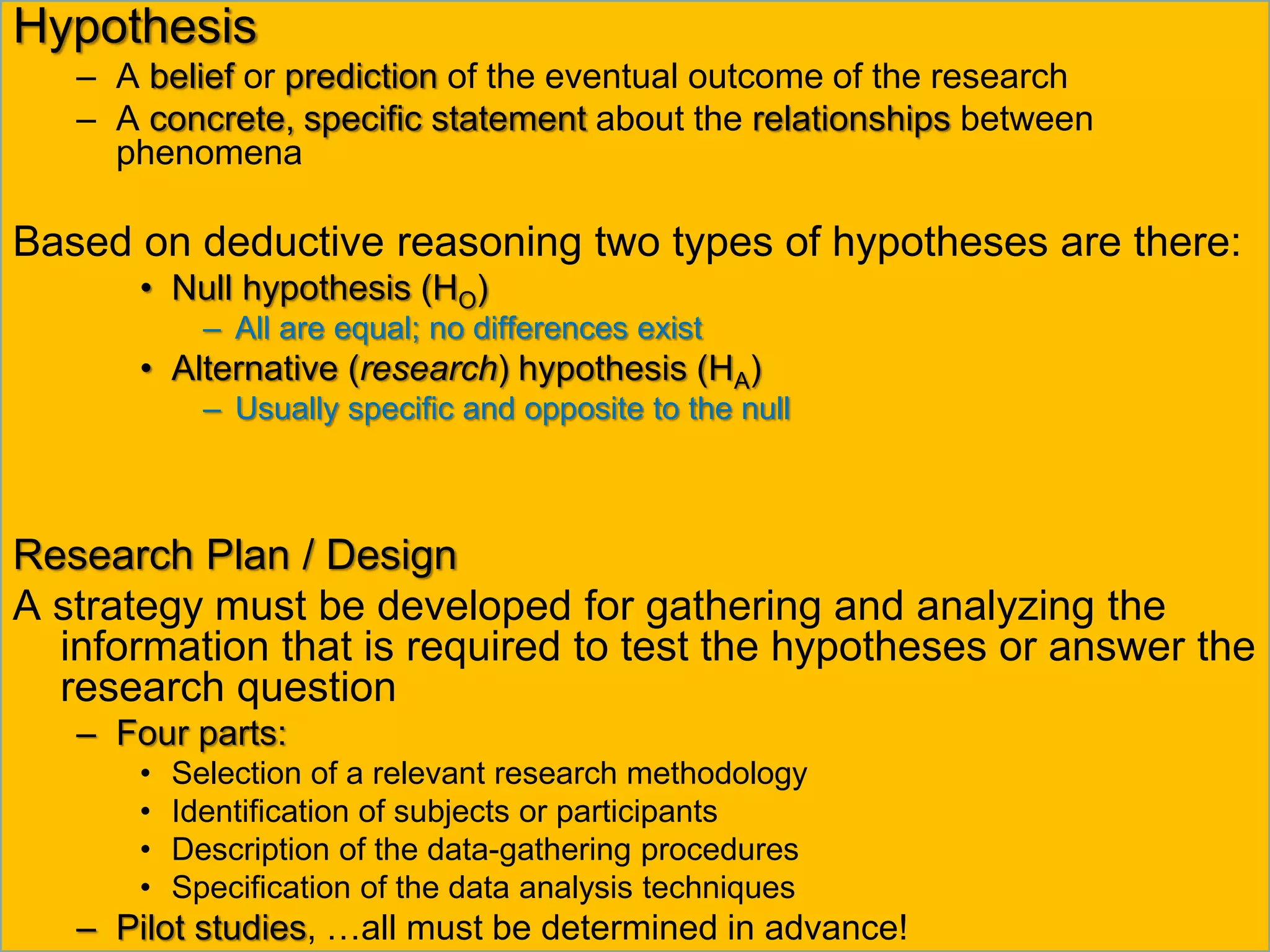
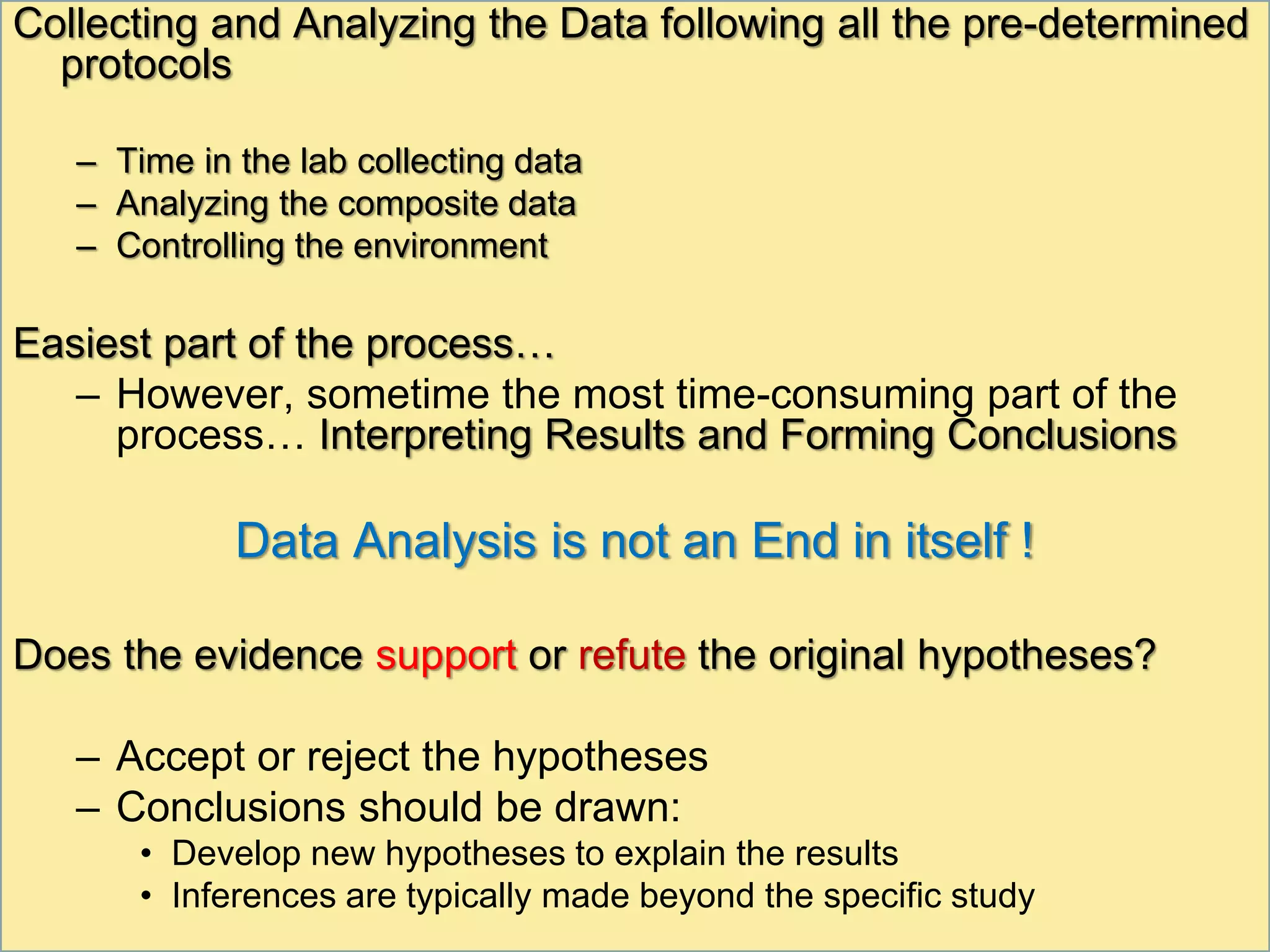
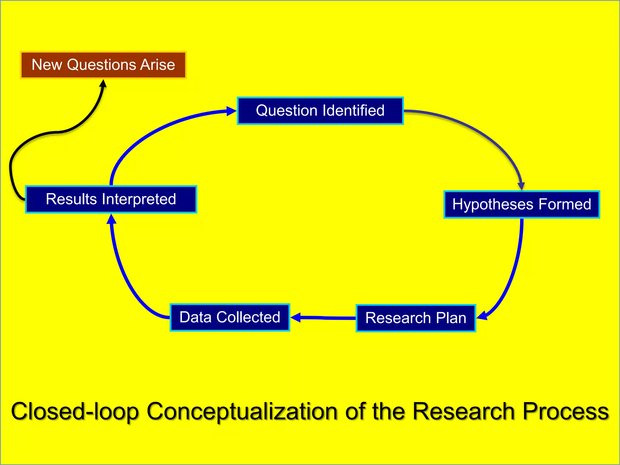
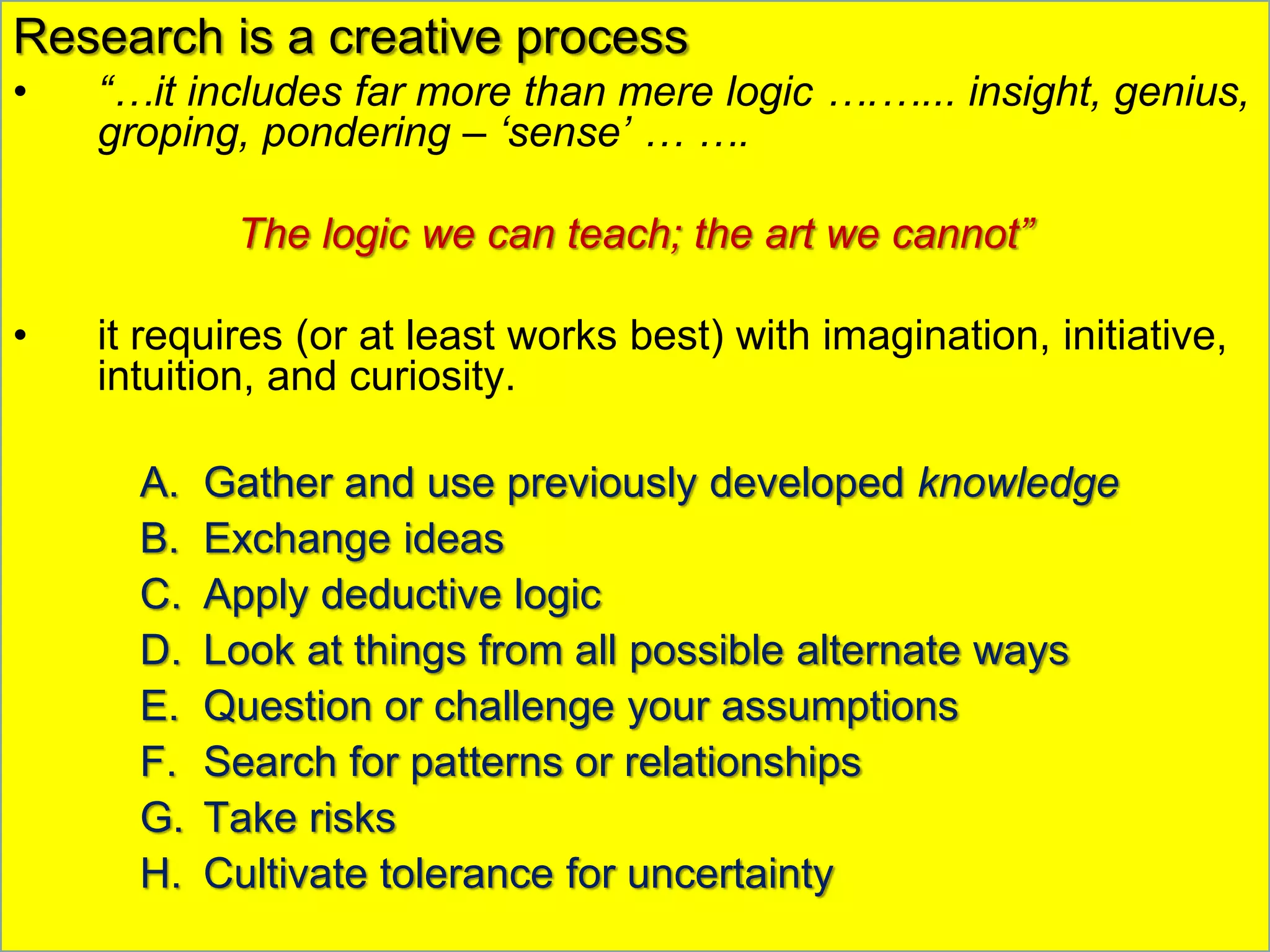
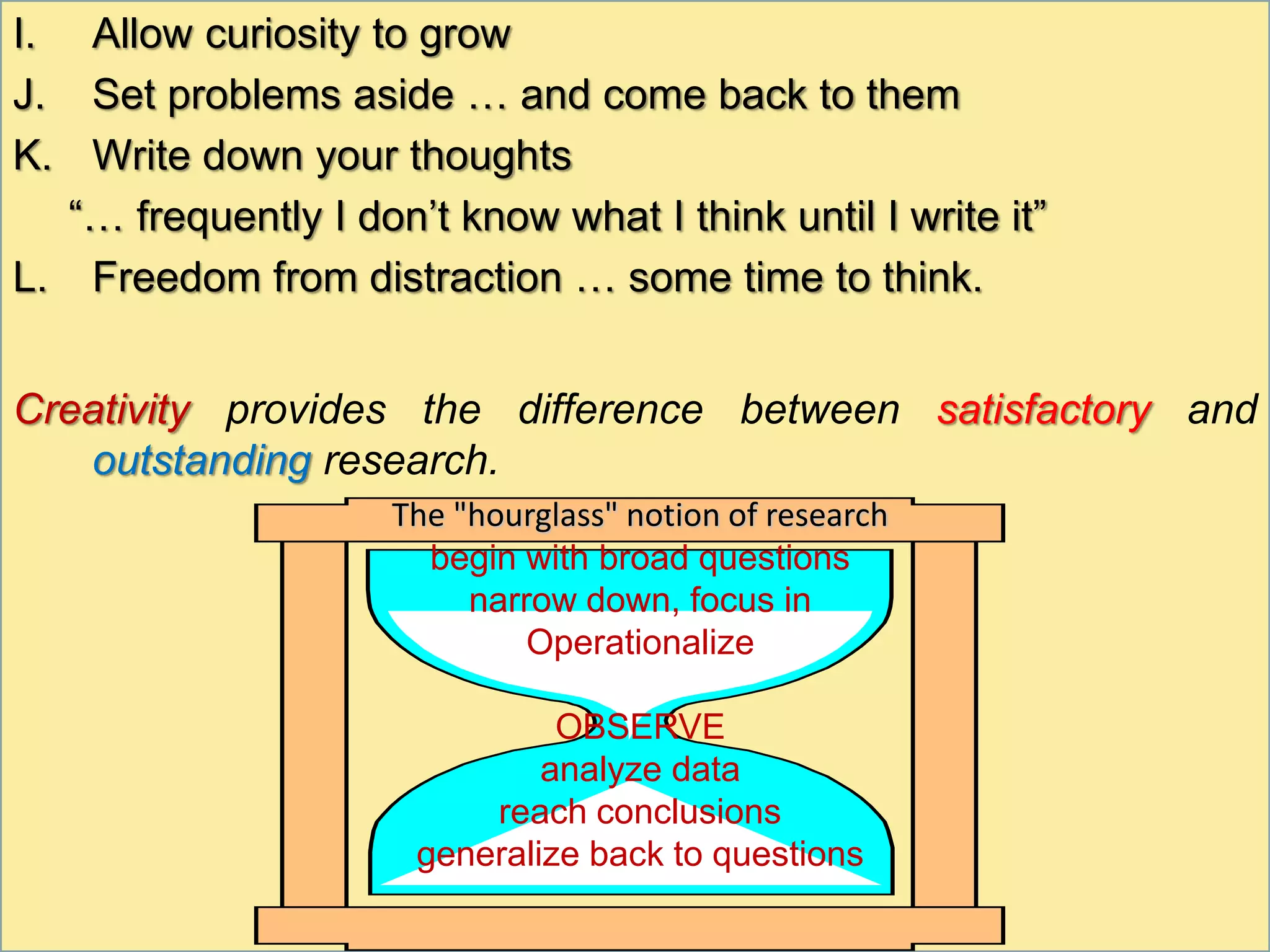
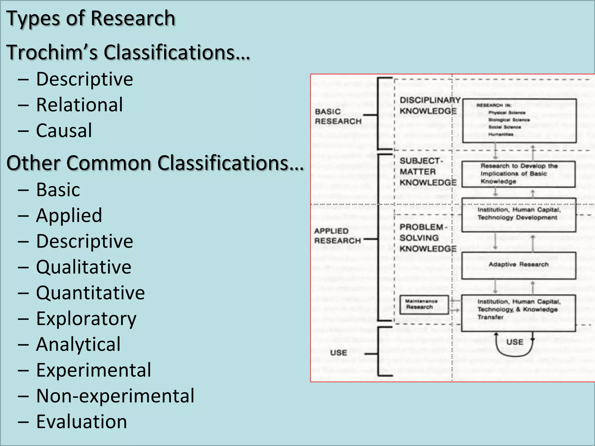
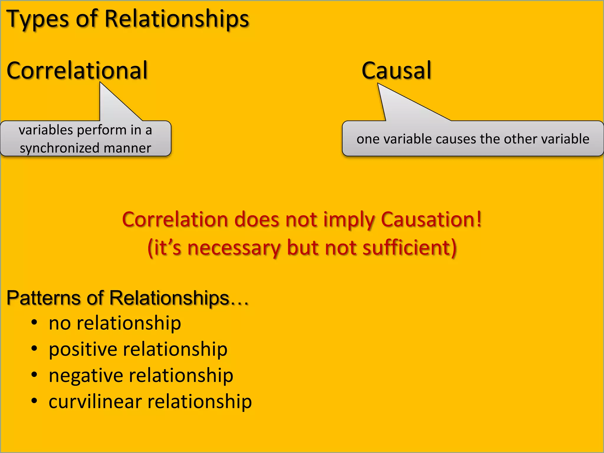
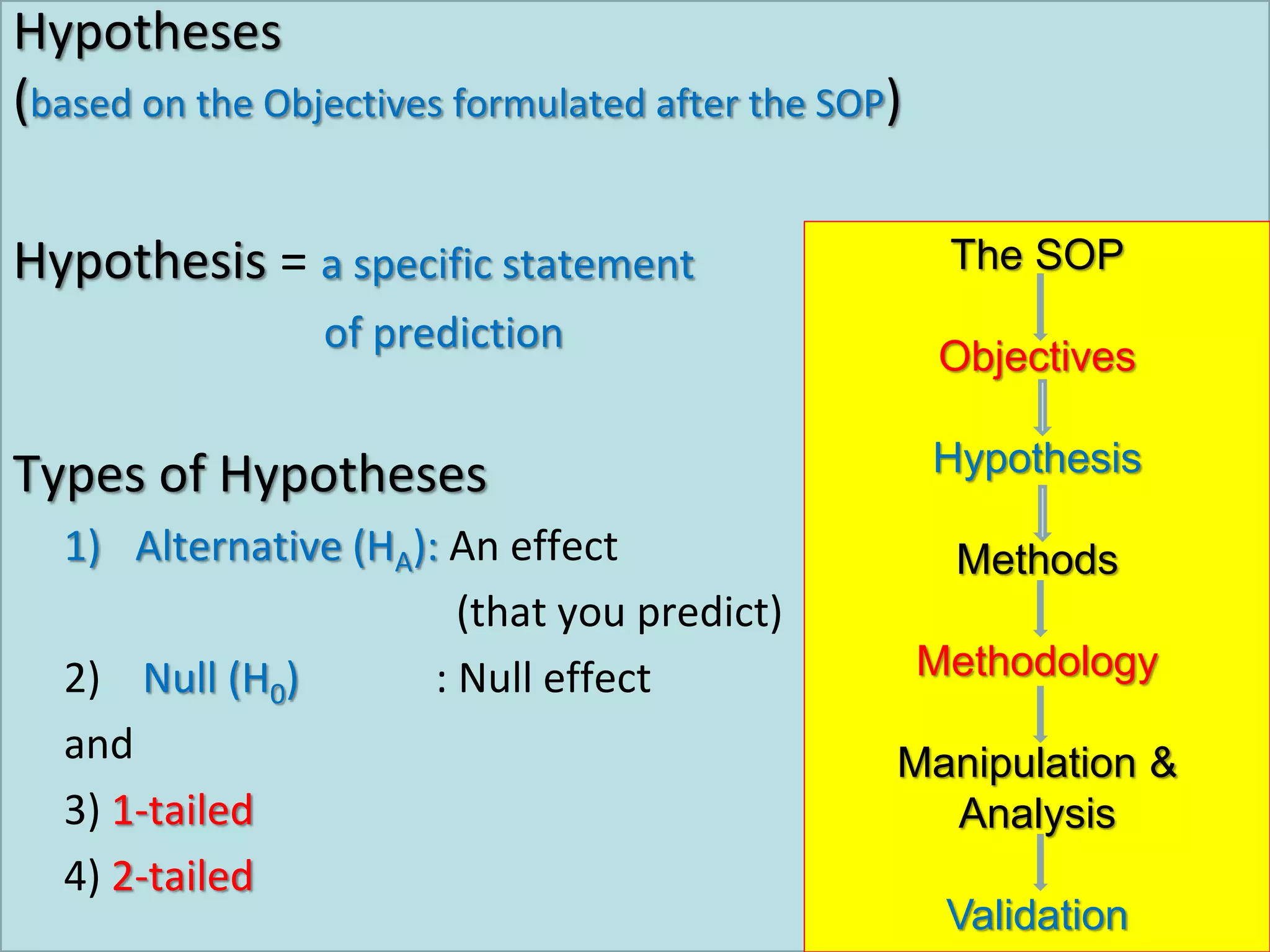
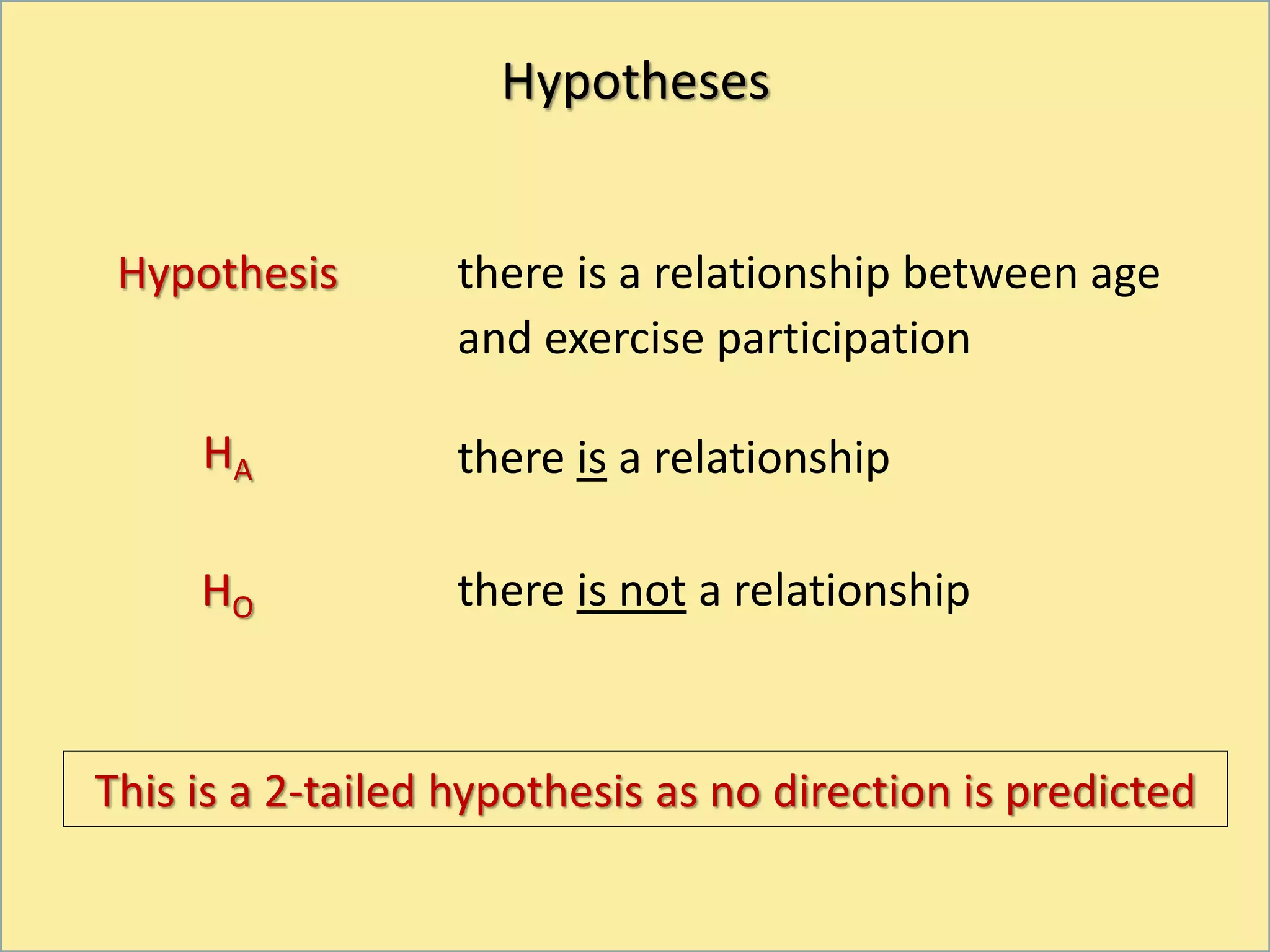
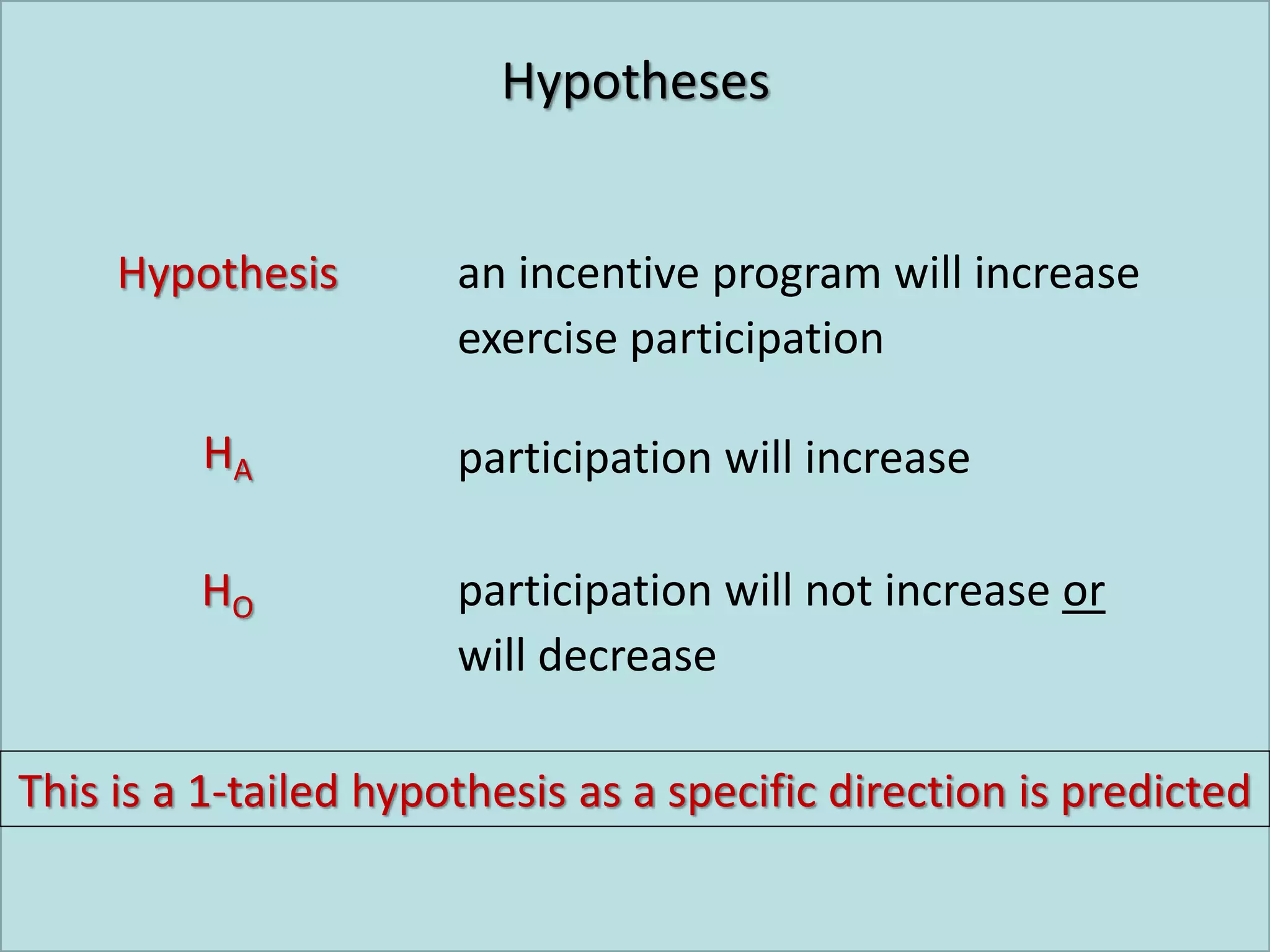
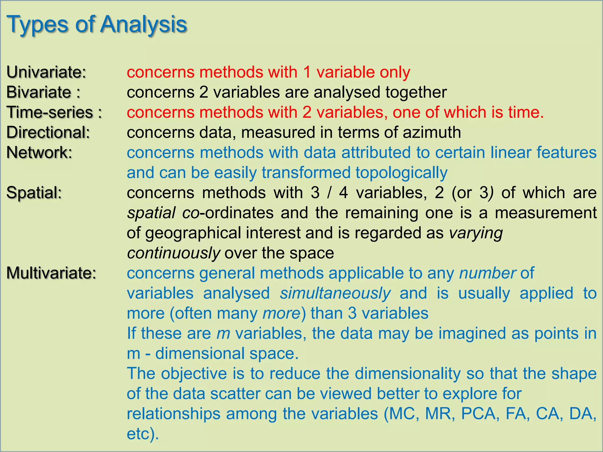
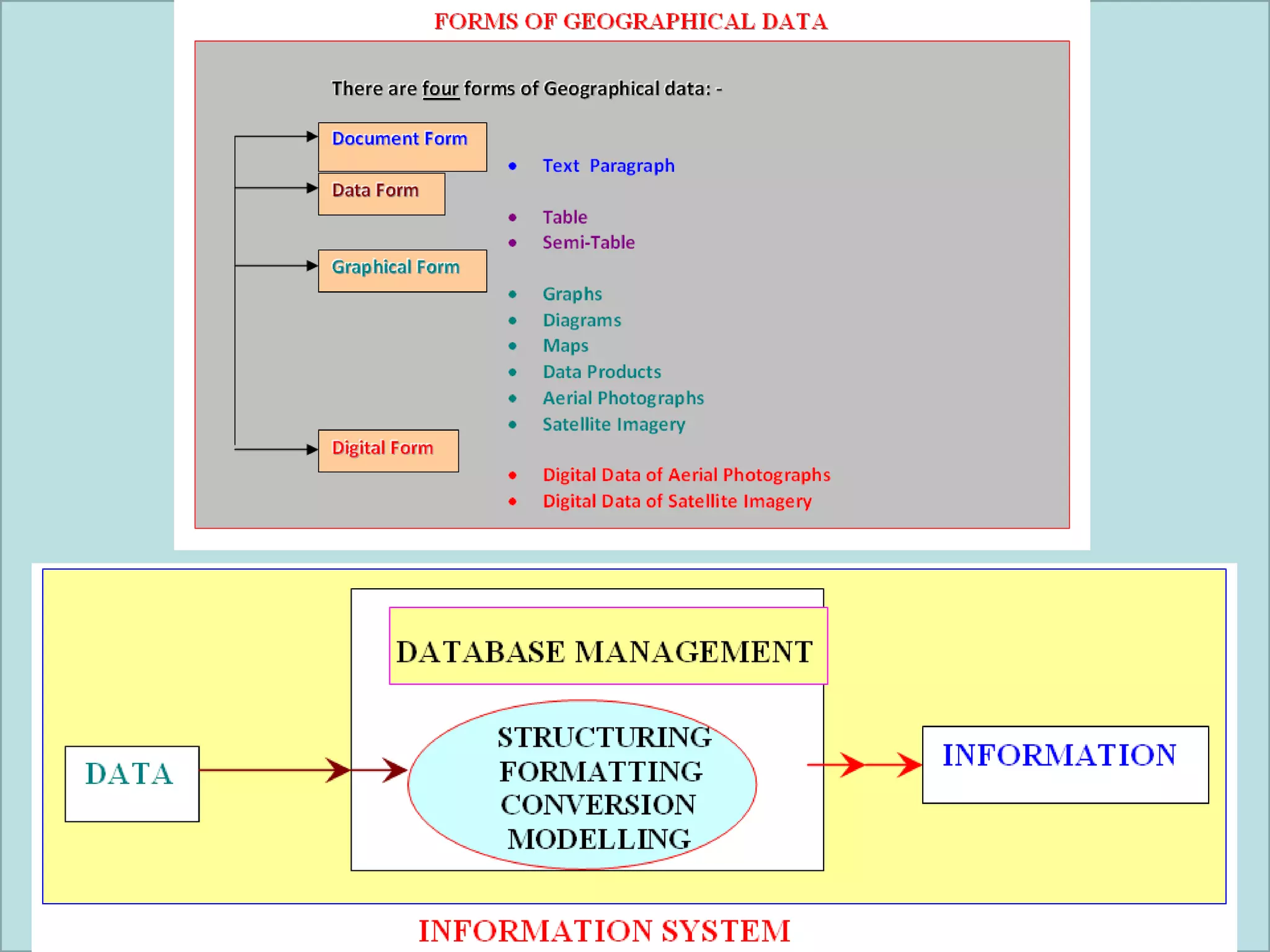
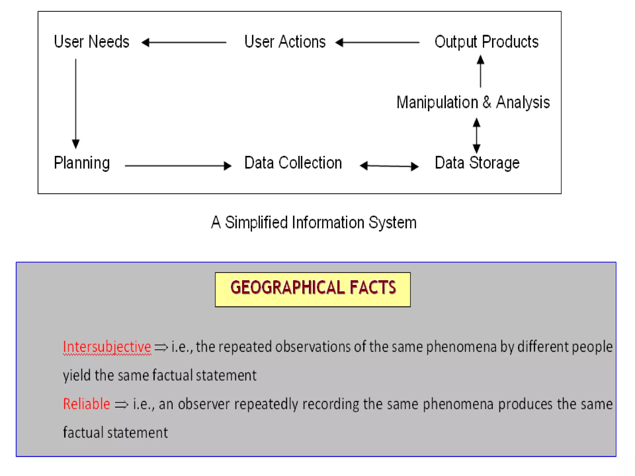
Research Issues and Concerns
Why Undertake Research?
• To investigate some existing situation or problem.
• To provide solutions to a problem.
• To explore and analyse more general issues.
• To construct or create a new procedure or system.
• To explain a new phenomenon.
• To generate new knowledge.
• A combination of two or more of any of the above.
(Hussey and Hussey 1997)
Geography seeks to answer the questions of why things are as
they are, and where they are.
The spatial pattern of geographical elements on the earth surface
seems to be apparently chaotic.
But, a deeper look into the pattern suggests that there is some
sort of spatial regularity or order that can be defined, identified
and analysed in space – time frame (i.e., measured, monitored,
mapped and modelled) with a scientific understanding of
geographical knowledge.
It is this that forms the philosophical foundation of the discipline of
Geography.
Naturally, it is the Geographer who discovers this spatial order,
the nature of which is analysed in space-time language
1. to identify the order-forming processes, and then
2. to comprehend and model its operational mechanism and lastly,
3. to examine the order-forming factors for scientific explanation.
The most comprehensible definition: “Geography…. deals with the
description and explanation of the areal differentiation of the
earth's surface ”.
The statement has two parts ―
1. The first part concerns: how one should study phenomena;
It includes the cognitive description and explanation
(cognitive = coherent, rational and realistic, description =
analysis of inter-connections within the geographical
objects / events, explanation = necessity of such inter-
connections). Thus, it refers to the methods of geography.
2. The second part concerns: what one should study; It
identifies a domain of objects and events defining the
operations of description and explanation. Thus, it
concerns the goals or objectives of geographical studies.
Therefore, the first half refers to the methods and second to the
goals or the substantive objectives of geographical study.
Hence lies the basis of the geographical (data) analysis:
the goal - oriented and object - specific
— descriptive,
— numerical (statistical, morphometric, cause-and-
effect, evolutionary, functional-and-ecological
and system),
— spatial, and
— cartographic analysis including its presentation
and geographical explanation.
Thus, methods come first, based on certain philosophical
principles of geography.
As methods without philosophy and philosophy without
methodology are both meaningless, the foundation of scientific
geography is essentially goal - oriented and object – specific, that
can be viewed multilaterally as –
 an activity,
 a process and
 an attempt at communicable understanding.
Geography beautifully blends the internal philosophies of both the
physical and social sciences to unravel the human drama, the
social fabric, dynamics of human life and civilization on earth.
Therefore, it provides a wealth of ideas to theorize about and
Geographers organize their thoughts around the following five
major themes, each one of which is, in its own way, provides an
operational definition of the nature of geography (Harvey, 1969)—
Areal Differentiation Theme: the traditional view in which the
geographers are primarily concerned with region
construction (Hartshrone, 1939).
Landscape Theme: the cultural geographers of the Berkeley
school carefully distinguished between the ‘natural’ and
the ‘cultural’ landscapes and examined their inter-
relationships (Sauer, 1925; Miller, 1949; James, Jones &
Wright, 1954).
Man-Environment Theme: emphasis on the study of man -
environments inter – relationships :: environmentalism,
possibilism, and probabilism (Semple, 1911; Vidal de la
Blache, 1922; Barrows, 1923; Brunhes,1925; Sorre,1947).
Spatial Distribution Theme: provides the framework for the study
of the structure and processes underlying a spatial
organisation of physical features / human activities in
which the question of when and where is the prime
objective (Marthe, 1877; Geer, 1923; Watson, 1955;
Bunge, 1962).
Geometric Theme: views geography as a synthetic combination
of the geometry of an infinite variety of spaces conceived
as 2D or 3D data layers of a geographer’s choice (gained
tremendous importance with the introduction of GIS/RS.
“…measure, measure and measure the differences of the differences of the
differences” is one Gallelian doctrine, which summarises well the mathematical-
philosophical base of the discipline of geography.
Geographical Analysis can be constructed in three ways ―
1. deductive-predictive approach (Braithwaite, 1960; Nagel, 1961 and
Hempel, 1965): based on the mechanistic principles of classical physics to
establish statements or laws governing the behaviour of various types of
events. The law then assumes the level of a universally true statement,
making prediction and explanation entirely symmetric.
2. relational approach: explanation is regarded as a matter of relating the
event to be explained to other events already experienced as these are all
connected together through a network (Ryle, 1949; Wisdom, 1952; Toulmin,
1960B; Bambrough, 1964; Workman, 1964 and Hanson, 1965).
3. model or analogy form of explanation (Workman,1964): an
unexpected occurrence can be made less unexpected by developing some
picture of events in such a way that the unfamiliar becomes or seems more
familiar. It may be used, by way of explanation, to render something difficult
or curious to comprehend into something, which is reasonably familiar.
These approaches are not at all mutually exclusive; all of them, however, are accepted
to be valid approaches to constructing a scientific explanation in given circumstances
The scientific statements about the real world are normally
ordered in a consistent hierarchy-
1) the lowest - order statements are called factual statements,
2) the intermediates are called generalizations or empirical laws and
3) the highest -order statements are called general or theoretical laws.
The prime aim of geographical research is to find the highest -
order transform of the lowest - order statements. There are
two different routes for this (Harvey, 1973) —
Route – I or ‘top down’ approach: starts from a set of initial conditions,
from which hypotheses are developed, and progresses, by reference to
empirical evidence and previously established laws, to reach logically
consistent conclusions.
Route – II or ‘bottom up’ approach: works in the opposite direction by
moving from the measurement and observation of phenomena, through a
process f ordering and classification, to the recognition of pattern and
regularity. Scientists, by these alternative routes, succeed in establishing
new deductive or inductive scientific laws.
Deduction and Induction
Deduction
Induction
11
The Process of Research
Thus, research is…
1. Searching for Explanation of events, relationships and causes
• What, how and why things occur
• Are there interactions?
2. A Process
• Planned and managed, scientific and systematic search for
something relevant to society and nation
• The process is creative
• It is circular: always leads to more questions
• an academic activity in the pursuit of truth,
• A voyage of discovery from the known to the unknown
• a search for knowledge: an original contribution to the existing stock
of knowledge, and
• an art of scientific investigation.
All well-designed and conducted research has potential
application.
Usually the ultimate goal is theory generation and verification.
Hypotheses
Theories
Laws
In an ideal
world…
Scientific Research has four
general characteristics —
1. it is empirical: based on
observation and reasoning,
2. it is theoretical: summarizes
data yielding precisely the
logical relationship between
propositions that explain causal
relationship,
3. it is cumulative: generalizations /
theories are corrected, rejected
and newly developed theories
are built upon one another.
4. it is non-ethical: scientists do not
comment whether certain things
/ events/ objects / phenomena /
systems / structures are good or
bad; they only explain them.
However, there are limits to the application of scientific methods in
geography that make geography a special kind of science with six
distinctive explanatory forms —
1) Cognitive description (i.e., how may the phenomena being studied
be ordered and grouped?),
2) Morphometric analysis (i.e., how are the phenomena organised in
terms of their spatial structure and form?),
3) Cause - and - effect analysis (i.e., how were the phenomena
caused?),
4) Evolutionary analysis (i.e., how did the phenomena originate and
develop?),
5) Functional and ecological analysis (i.e., how do the particular
phenomena relate to and interact with phenomena in
general?), and
6) System analysis (i.e., how are the phenomena organised as a
coherent system?).
However, there may be overlaps, and synthetic approaches (like, genetic –
classificatory, genetic – morphological, genetic – system and so on) can be
easily developed and applied. However, the choice of form depends entirely
upon the kind of question asked.
Aristotle: laid the foundation of the 1st Paradigm to guide
Research Process
1. It is necessary to establish the necessary characteristics / nature of
the events / phenomenon being investigated
2. It is necessary to identify the substance of which it is composed
3. It is necessary to identify the process through which the
phenomenon has attained its form
4. It is necessary to identify the purpose that the phenomenon
concerned fulfills I the overall scheme of nature
Essentially a Scientific Procedure comprising:
– the observation,
– identification,
– investigation, and
– theoretical explanation of natural phenomenon
Research Methods (Methodology = Science of Methods)
– the ways one collects and analyzes data
– methods developed for acquiring trustworthy knowledge via reliable
and valid procedures
Methodology – the study of the general approach to inquiry in a
given field
Method – the specific techniques, tools
or procedures applied
to achieve a given
objective
The Scientific Method
– Identifying the problem (SOP)
– Formulating a hypothesis (OH)
– Developing the research plan (RD)
– Collecting and analyzing the data (GDM)
– Interpreting results and forming
conclusions (ECR)
Identifying the Problem
– Several sources
– Theoretical basis
– Professional practice
– Personal experience
– Shear curiosity
– Starts as a broad question that must be narrowed
– Problem statement; experimental approach to the problem; etc.
Three categories when selecting a research problem -
– Those who know precisely what they want to do and have a well
conceived problem
– Those who have many interest areas and are having difficulty deciding
exactly what they want to study
– Those who do not have any idea about a worthwhile research problem
Hypothesis
– A belief or prediction of the eventual outcome of the research
– A concrete, specific statement about the relationships between
phenomena
Based on deductive reasoning two types of hypotheses are there:
• Null hypothesis (HO)
– All are equal; no differences exist
• Alternative (research) hypothesis (HA)
– Usually specific and opposite to the null
Research Plan / Design
A strategy must be developed for gathering and analyzing the
information that is required to test the hypotheses or answer the
research question
– Four parts:
• Selection of a relevant research methodology
• Identification of subjects or participants
• Description of the data-gathering procedures
• Specification of the data analysis techniques
– Pilot studies, …all must be determined in advance!
Collecting and Analyzing the Data following all the pre-determined
protocols
– Time in the lab collecting data
– Analyzing the composite data
– Controlling the environment
Easiest part of the process…
– However, sometime the most time-consuming part of the
process… Interpreting Results and Forming Conclusions
Data Analysis is not an End in itself !
Does the evidence support or refute the original hypotheses?
– Accept or reject the hypotheses
– Conclusions should be drawn:
• Develop new hypotheses to explain the results
• Inferences are typically made beyond the specific study
New Questions Arise
Results Interpreted
Data Collected
Question Identified
Hypotheses Formed
Research Plan
Closed-loop Conceptualization of the Research Process
Research is a creative process
• “…it includes far more than mere logic ….…... insight, genius,
groping, pondering – ‘sense’ … ….
The logic we can teach; the art we cannot”
• it requires (or at least works best) with imagination, initiative,
intuition, and curiosity.
A. Gather and use previously developed knowledge
B. Exchange ideas
C. Apply deductive logic
D. Look at things from all possible alternate ways
E. Question or challenge your assumptions
F. Search for patterns or relationships
G. Take risks
H. Cultivate tolerance for uncertainty
I. Allow curiosity to grow
J. Set problems aside … and come back to them
K. Write down your thoughts
“… frequently I don’t know what I think until I write it”
L. Freedom from distraction … some time to think.
Creativity provides the difference between satisfactory and
outstanding research.
The "hourglass" notion of research
begin with broad questions
narrow down, focus in
Operationalize
OBSERVE
analyze data
reach conclusions
generalize back to questions
Types of Research
Trochim’s Classifications…
– Descriptive
– Relational
– Causal
Other Common Classifications…
– Basic
– Applied
– Descriptive
– Qualitative
– Quantitative
– Exploratory
– Analytical
– Experimental
– Non-experimental
– Evaluation
Variable Attribute
any observation that can a specific value on a variable
take on different values
Example:
Age 18, 20, 30 years
Gender Male , Female
Satisfaction 1 = Very Satisfied 2 = Satisfied 3 = Somewhat Satisfied
4 = Not Satisfied 5 = Not Satisfied at all
Independent Variable (IV)…
what you (or nature) manipulates in some way (x)
Dependent Variable (DV)…
what you presume to be influenced by the IV (y)
Slope
Discharge
Cross-section
Bed Roughness
IV = x
Velocity
DV = y
Types of Relationships
Correlational Causal
Correlation does not imply Causation!
(it’s necessary but not sufficient)
Patterns of Relationships…
• no relationship
• positive relationship
• negative relationship
• curvilinear relationship
variables perform in a
synchronized manner
one variable causes the other variable
Hypotheses
(based on the Objectives formulated after the SOP)
Hypothesis = a specific statement
of prediction
Types of Hypotheses
1) Alternative (HA): An effect
(that you predict)
2) Null (H0) : Null effect
and
3) 1-tailed
4) 2-tailed
The SOP
Objectives
Hypothesis
Methods
Methodology
Manipulation &
Analysis
Validation
Hypotheses
Hypothesis there is a relationship between age
and exercise participation
HA there is a relationship
HO there is not a relationship
This is a 2-tailed hypothesis as no direction is predicted
Hypotheses
Hypothesis an incentive program will increase
exercise participation
HA participation will increase
HO participation will not increase or
will decrease
This is a 1-tailed hypothesis as a specific direction is predicted
Types of Analysis
Univariate: concerns methods with 1 variable only
Bivariate : concerns 2 variables are analysed together
Time-series : concerns methods with 2 variables, one of which is time.
Directional: concerns data, measured in terms of azimuth
Network: concerns methods with data attributed to certain linear features
and can be easily transformed topologically
Spatial: concerns methods with 3 / 4 variables, 2 (or 3) of which are
spatial co-ordinates and the remaining one is a measurement
of geographical interest and is regarded as varying
continuously over the space
Multivariate: concerns general methods applicable to any number of
variables analysed simultaneously and is usually applied to
more (often many more) than 3 variables
If these are m variables, the data may be imagined as points in
m - dimensional space.
The objective is to reduce the dimensionality so that the shape
of the data scatter can be viewed better to explore for
relationships among the variables (MC, MR, PCA, FA, CA, DA,
etc).
Identification
of
Problem Area/Deficit Area/Negative Area
through
‘Spatial Mapping / Trend Surface Mapping’
using
‘indices’
Derived from Statistical Analysis
Data Acquisition
Physical Database
application of RS / GIS technology
Socio-economic Database
GDM using attribute Data
Mapping
Thematic Data Layers (physical)
Thematic Data Layers (social)
Thematic Data Layers (economic)
Data Integration
using RS/GIS technology adopting appropriate
project design and management with
proper process models.
Statistical Techniques: Exploratory Techniques
Analysis of ‘dependence’
Multiple Regression
Analysis of ‘interdependence’
Principal Component Analysis
Factor Analysis
‘Classification’
Discriminant Analysis
Cluster Analysis
using PC Scores / Factor Scores)
Statistical Packages are now readily available for the
Geographers for such applications.
Exploratory techniques do suggest, rather than do test
hypotheses.
1.It provides extra information if variables are
correlated with each other.
2.It brings out the structure of the data
scatter in multivariate space.
3.If there is no significant correlation,
variables are dealt separately.
However, these are commonly overlooked mainly because of:
1. blind adherence to traditional procedures,
2. inadequate knowledge in mathematics and statistics,
3. not risking the data exploration.
Modern Geographers are more equipped with basic knowledge
in mathematics, statistics, and computer.
Example – 1: Analysis of Dependence
Objective: To determine the relationship between a variable
of interest and a set of exploratory variables.
Multivariate / Multiple Linear Regression Model (MLRM)
It involves the specification and identification of the type and nature of
dependence of a single variable upon a set of controlling, predictor or
explanatory variables.
The basic postulate is that the variation in the Dependent Variable is made up
of two parts —
one, deterministically related to the explanatory variables not
included in the regression model,
and, the effects of measurement error (random variation).
Hence, the random term (called, disturbance term, when the regression
model applied to a population and residual term, when applied to a
sample) is often assumed to be normally distributed.
Parameter Mini
mum
Maxi
mum
Mean Standard
Deviation
Vari-
ance
Skew
ness
Kurtosis
HI: Hypsometric integral 0.154 0.630 0.370 0.130 0.017 0.132 -1.058
L / W ratio 1.207 3.260 2.057 0.534 0.285 0.553 -0.164
CR: Circularity ratio 0.364 0.847 0.549 0.104 0.011 0.385 0.082
ER: Elongation ratio 0.473 0.793 0.624 0.064 0.004 0.024 0.740
CC: Compactness coefficient 1.087 1.659 1.368 0.131 0.017 0.270 -0.525
FF : Form factor 0.176 0.494 0.309 0.063 0.004 0.418 0.947
BR : Basin relief (m) 7.000 343.00 105.802 86.620 7503.0 1.105 0.177
θ : Basin slope (degree) 0.009 0.190 0.038 0.037 0.001 2.153 5.588
DI : Dissection Index 0.163 0.940 0.498 0.176 0.031 0.228 -0.269
RI : Ruggedness index 0.012 0.635 0.161 0.167 0.028 1.265 0.848
SF : Stream frequency (No./ sq km) 0.139 5.893 1.563 1.301 1.693 1.136 1.241
Dd : Drainage density (km / sq km) 0.416 2.677 1.369 0.640 0.410 0.379 -1.053
DT : Drainage texture 0.058 13.521 2.878 3.219 10.361 1.382 1.616
Descriptive Measures: 43 Sub-basins of Dulung basin
HI L/W CR ER CC FF BR θ DI RI SF Dd DT
HI 1
L/W -0.23 1
CR 0.55 -0.39 1
ER 0.36 -0.81 0.65 1
CC -0.56 0.37 -0.99 -0.63 1
FF 0.36 -0.80 0.65 0.99 -0.62 1
BR -0.78 0.06 -0.70 -0.23 0.73 -0.23 1
θ -0.57 0.03 -0.53 -0.21 0.55 -0.22 0.78 1
DI -0.63 0.31 -0.73 -0.42 0.72 -0.43 0.84 0.56 1
RI -0.72 -0.02 -0.60 -0.21 0.61 -0.21 0.86 0.70 0.63 1
SF -0.08 -0.29 0.00 0.11 -0.01 0.11 0.12 0.28 -0.21 0.44 1
Dd -0.32 -0.21 -0.16 -0.02 0.15 -0.02 0.30 0.41 -0.02 0.65 0.91 1
DT -0.12 -0.24 -0.03 0.06 0.02 0.06 0.15 0.30 -0.15 0.49 0.98 0.91 1
Correlation Matrix: 13 Morphometric Parameters
Model Summary
Correlation Coefficient, r = 0.84
Goodness of Fit, R2 = 0.71
Standard Error of Estimate, SE = 0.076
Durbin – Watson Coefficient = 1.275
Sum of
Squares
df Mean
Square
F Sig.
Regression 0.509757 7 0.072822 12.5394 6.45E-08
Residual 0.203262 35 0.005807
Total 0.713019 42
ANOVA
Unstandardized Coefficients Standardized
Coefficients
t Significance
β Std. Error βs
-0.13975 1.16389 -0.12007 0.90511
-0.16784 0.71854 -0.13445 -0.23359 0.81666
0.26056 0.56572 0.26146 0.46057 0.64795
1.00431 0.29835 0.48252 3.36618 0.00186
-0.00205 0.00055 -1.35962 -3.70638 0.00072
0.82220 0.53227 0.23536 1.54469 0.13141
0.25929 0.16109 0.34968 1.60959 0.11647
-0.05855 0.15242 -0.07488 -0.38416 0.70318
The multivariate linear regression model is represented by the equation —
HI = — 0.13975 — 0.13445 CR + 0.26146 CC + 0.48252FF —
1.35962 BR + 0.23536 θ +0.34968 DI — 0.07488 RI
Regression Parameters
Example – 2: Analysis of Interdependence
It is performed via two approaches — principal components
analysis (PCA) and factor analysis (FA).
PCA provides a means of eliminating redundancies from a set of
interrelated variables and the resulting principal components
are uncorrelated.
FA, on the other hand, is a method of investigating the
correlation structure of a multivariate system.
Thus, it is an attempt to find groups of variables (factors)
measuring a single important aspect of the system.
As these factors are not necessarily uncorrelated, a method of
transforming the factors (called, rotation) is applied.
This involves a prior hypothesis that the system has a simple
structure and the factors are rotated to fit this as closely as
possible.
Factor Analysis (FA)
It interpreting the structure of the variance-covariance matrix from a collection of
multivariate observations.
As the variables measured may not all be directly comparable, all of them are
converted to standardized form. Hence, the transformed values have zero mean
and unit variance.
In geographic research, it is the most important technique in multivariate problems,
as —
1. ideas summarising the relationships among the components of a system of
interacting variables can be formed,
2. the common characteristics of the variables, that cause their intercorrelation
and explains their differences in characteristics can be identified.
3. eigen values and eigen vectors can be extracted.
4. structure of the variance - covariance matrix can be efficiently interpreted.
5. the most diagnostic and significant variable(s) in terms of factor loadings in
the multivariate system can be identified and
6. factor score values can be used as a criterion of differentiation between and
among the samples in multivariate space.
Variable Minimum Maximum Mean Stand_D Variance Skewness Kurtosis
x2 4.77 97.81 54.89 18.36 337.24 -0.23 0.02
x3 0 76.35 20.63 20.45 418.03 1.32 0.70
x4 0.10 4.28 1.64 1.04 1.09 0.22 -0.66
x5 1.08 6.87 3.12 1.44 2.08 0.90 0.15
x6 2.49 33.51 6.27 4.55 20.69 4.51 23.79
x7 1.13 11.15 2.21 1.29 1.67 5.68 38.94
x8 817.96 1062.50 964.64 37.87 1434.13 -0.59 3.43
x9 1.06 86.38 49.53 18.47 341.09 -0.72 0.37
x10 0 45.11 11.14 9.91 98.15 1.14 1.36
x11 13.15 96.62 39.34 20.40 416.33 1.06 0.42
x12 17.78 64.33 50.97 8.67 75.09 -1.22 2.47
x13 33.30 57.55 47.52 5.68 32.31 -0.29 -0.37
x14 0 8.23 1.99 1.21 1.46 2.53 11.70
x15 0 27.75 6.00 8.27 68.34 1.26 0.30
x16 0 63.47 4.50 8.49 72.01 5.87 40.00
x17 0 27.76 3.41 5.37 28.83 2.99 10.54
x18 0 27.55 4.44 7.03 49.42 1.73 2.18
x19 2.58 66.83 25.80 10.79 116.37 0.94 2.85
x20 27.15 81.89 53.39 11.66 136.04 0.34 0.23
x21 0 22.14 5.15 4.49 20.12 1.71 3.56
x22 0 60.83 15.65 11.04 121.99 1.77 4.50
Descriptive Statistics: 21 Variables
x2 x3 x4 x5 x6 x7 x8 x9 x10 x11 x12 x13 x14 x15 x16 x17 x18 x19 x20 x21
x2 1
x3 0.35 1
x4 0.40 0.19 1
x5 0.62 0.39 0.61 1
x6 -0.39 0.02 0.24 0.32 1
x7 -0.37 0.17 -0.06 0.06 0.67 1
x8 0.16 0.12 0.12 -0.01 -0.20 -0.10 1
x9 0.17 -0.05 0.37 0.22 0.03 -0.32 -0.05 1
x10 0.58 0.53 0.38 0.69 0.02 -0.01 -0.11 -0.06 1
x11 -0.43 -0.21 -0.52 -0.54 -0.03 0.29 0.10 -0.87 -0.43 1
x12 0.25 0.13 0.61 0.37 0.11 -0.15 -0.05 0.67 0.17 -0.69 1
x13 -0.07 0.11 -0.18 -0.44 -0.40 0.03 0.25 -0.32 -0.16 0.37 -0.21 1
x14 0.03 -0.03 -0.07 -0.07 -0.21 -0.25 -0.32 0.26 0.00 -0.24 0.38 0.03 1
x15 0.23 0.23 0.25 0.18 -0.08 -0.10 0.12 0.04 0.26 -0.16 0.43 -0.04 0.31 1
x16 0.06 -0.05 0.11 0.28 0.05 -0.04 -0.05 0.04 0.27 -0.16 0.05 -0.10 0.22 -0.01 1
x17 0.28 0.31 0.27 0.18 -0.10 -0.06 0.23 0.19 0.26 -0.30 0.30 0.04 0.21 0.48 0.01 1
x18 0.01 0.21 0.16 -0.06 -0.13 -0.10 0.14 0.10 0.04 -0.11 0.33 0.15 0.10 0.36 0.04 0.09 1
x19 0.04 0.19 -0.07 -0.16 -0.03 0.41 0.13 -0.02 -0.15 0.09 0.16 0.26 0.16 0.19 -0.20 0.35 0.11 1
x20 0.07 -0.10 -0.37 -0.23 -0.45 -0.21 0.03 -0.36 -0.04 0.34 -0.46 0.25 -0.26 -0.29 -0.09 -0.27 -0.06 -0.40 1
x21 0.02 0.04 0.06 0.16 0.07 -0.12 -0.18 0.00 0.31 -0.15 -0.05 -0.04 0.20 0.04 0.51 0.01 -0.03 -0.36 -0.15
x22 -0.12 -0.09 0.44 0.34 0.48 -0.13 -0.08 0.40 0.05 -0.39 0.35 -0.50 0.04 0.10 0.08 -0.06 -0.04 -0.41 -0.61 0.1
Correlation Matrix: 21 x 21 Matrix
Factor Extraction through PCA
Variable Communality Compo-
nent Initial Eigenvalues Extraction Sums of Squared Loadings Rotation Sums of Squared Loadings
Initial Extraction
Total
% of
Variance Cumulative % Total
% of
Variance Cumulative % Total
% of
Variance Cumulative %
X2 1.000 .842 1 4.979 23.708 23.708 4.979 23.708 23.708 3.949 18.806 18.806
X3 1.000 .624 2 2.817 13.414 37.123 2.817 13.414 37.123 2.964 14.114 32.920
X4 1.000 .688 3 2.377 11.321 48.443 2.377 11.321 48.443 2.479 11.806 44.726
X5 1.000 .884 4 2.238 10.658 59.102 2.238 10.658 59.102 2.099 9.995 54.720
X6 1.000 .908 5 1.693 8.063 67.165 1.693 8.063 67.165 1.842 8.773 63.494
X7 1.000 .872 6 1.237 5.892 73.057 1.237 5.892 73.057 1.636 7.790 71.284
X8 1.000 .858 7 1.010 4.809 77.866 1.010 4.809 77.866 1.382 6.583 77.866
X9 1.000 .831 8 .944 4.497 82.363
X10 1.000 .862 9 .720 3.428 85.791
X11 1.000 .858 10 .633 3.016 88.807
X12 1.000 .818 11 .564 2.685 91.492
X13 1.000 .565 12 .439 2.093 93.585
X14 1.000 .798 13 .364 1.732 95.317
X15 1.000 .596 14 .281 1.339 96.655
UNROTATED ROTATED
1 2 3 4 5 6 7 1 2 3 4 5 6 7
X2 .509 .535 -.391 .177 -.228 -.232 .083 .191 .744 -.463 .129 -.034 -.076 .116
X3 .333 .405 .053 .543 .062 -.046 -.214 -.123 .680 .118 .221 -.075 .280 .017
X4 .736 -.020 .043 .154 -.254 .234 .038 .588 .422 .139 -.007 .049 .203 .319
X5 .747 -.079 -.267 .475 -.119 -.094 .006 .417 .791 .195 -.092 .159 -.082 .073
X6 .201 -.740 .354 .431 .041 .062 -.050 .233 .011 .909 -.132 .049 -.081 -.027
X7 -.187 -.311 .516 .655 .164 -.131 -.039 -.307 .073 .831 .220 -.145 -.085 -.071
X8 -.044 .398 .120 .120 -.406 .535 .466 -.069 -.011 -.155 .180 -.069 .093 .885
X9 .643 -.120 .110 -.544 -.233 -.177 .095 .870 -.061 -.209 .115 -.070 -.025 -.091
X10 .560 .219 -.411 .523 .167 -.102 -.142 .047 .877 .003 -.036 .275 .080 -.092
X11 -.854 .002 .099 .239 .130 .210 -.017 -.810 -.370 .188 -.087 -.071 -.016 .127
X12 .774 .078 .314 -.292 -.052 -.009 -.164 .748 .155 -.024 .249 -.070 .394 -.110
X13 -.441 .541 .118 .000 .153 .181 .091 -.545 -.156 -.266 .302 -.028 .211 .192
X14 .271 .163 .112 -.503 .607 -.247 -.050 .232 -.163 -.266 .419 .331 .218 -.560
X15 .438 .399 .275 -.013 .240 .275 -.190 .164 .203 -.032 .331 .110 .636 .033
X16 .251 -.127 -.367 .038 .554 .212 .291 .042 .106 -.002 -.007 .799 -.031 -.015
X17 .424 .478 .283 .075 .115 -.028 .342 .188 .269 -.108 .659 .098 .131 .212
X18 .186 .345 .225 -.134 .095 .510 -.550 .024 .011 -.075 -.037 -.074 .883 .031
X19 -.045 .390 .750 .140 .122 -.321 .178 -.127 -.032 .182 .849 -.329 .058 -.041
X20 -.550 .289 -.573 .005 -.218 -.074 -.245 -.556 .085 -.504 -.443 -.208 -.127 -.037
X21
.219 -.167 -.438 .030 .633 .225 .189 -.007 .102
5.99E-
005
-.099 .851 .016 -.110
X22 .536 -.619 .051 -.154 -.146 .300 .008 .714 -.100 .354 -.321 .196 .070 .123
Component Matrix: Loadings
Factor Score Matrix
GP F1 F2 F3 GP F1 F2 F3
1 -1.410 -0.328 -0.100 32 0.538 -0.519 0.289
2 0.914 0.241 -0.389 33 -0.380 2.456 0.496
3 -0.888 3.086 -0.203 34 0.876 -0.564 -0.552
4 0.003 0.200 -0.512 35 0.415 0.675 -0.321
5 0.074 0.050 -0.506 36 0.029 2.387 0.575
6 -0.092 0.833 -0.157 37 0.364 1.597 0.266
7 1.421 1.657 0.400 38 0.456 -0.492 -1.052
8 -0.984 -0.957 0.657 39 -1.297 -1.151 -0.753
9 -0.086 1.744 -0.101 40 -0.573 -1.146 0.676
10 0.566 1.215 -0.091 41 -1.089 -0.875 -0.315
11 0.597 0.525 -0.091 42 -0.101 0.077 -0.488
12 0.509 0.185 0.270 43 -2.006 -0.57 0.127
13 0.478 1.162 0.481 44 -0.133 -2.007 -1.132
14 0.001 0.312 -0.228 45 1.256 -0.339 0.932
15 0.177 0.213 -0.087 46 -1.231 -0.447 -0.600
16 0.198 0.569 -0.146 47 -0.186 0.557 -0.900
17 1.310 -0.362 -0.323 48 0.383 0.158 -0.120
18 0.435 0.002 -0.294 49 -1.333 -0.709 0.266
19 0.369 0.455 0.150 50 -1.54 -1.015 0.086
20 0.185 0.282 -0.653 51 -0.299 0.505 -0.521
21 -0.514 -0.361 -1.055 52 0.129 -0.59 -0.573
22 1.163 0.337 0.667 53 0.472 -0.21 -0.429
Output of Factor Analysis
1. The data comprise 21 socio-economic attributes of 61 GPs of
the Dulung basin.
2. The correlation matrix shows the significant relations at 0.01
level.
3. First four Factors emerged significant, together explaining
77.87% of the total variance.
4. Initially, x12, x5, x4, x9 had high positive loading and x11 high
negative loading on Factor – 1; x13 had high positive loading
and x22, x6 had high negative loading on Factor – 2.
After Varimax rotation,
1. x9, x12 and x22 have high positive loading and x11 high
negative loading on Factor – 1;
2. x10, xs, x2 and x3 have high positive loading on Factor – 2;
3. x6 and x7 have high positive loading on Factor – 3;
4. x19 has high positive loading on Factor – 4.
With respect to Factor – 1,
1. very high positive scores emerged in case of 9 basins;
2. basins with positive scores =35;
3. basins with negative score = 26; and
4. basins with very high negative scores = 9.
With respect to Factor – 2,
1. very high positive scores emerged in case of 9 basins;
2. basins with positive scores =28;
3. basins with negative score = 33; and
4. basins with very high negative scores = 7.
Factor Score – 1 may form the basis of Numerical
Classification of the GPs in terms of the 21
variables.
Range of
Factor Score
– 1
No. of Gram
Panchayats
Gram Panchayat
ID
Remarks
>2 1 61 Highly Developed
1 to 2 8 7, 55, 17, 45, 22, 27, 31, 26 Fairly Developed
0 to 1 26 2, 34, 23, 25, 11, 10, 32, 12, 13, 53,
38, 18, 35, 48, 19, 37, 16, 20, 15,
52, 28, 5, 58, 36, 4, 14
Developed
-1 to 0 17 6, 42, 44, 47, 29, 51, 59, 60, 33, 56,
24, 21, 40, 3, 54, 8
Backward
-2 to -1 6 41, 46, 39, 49, 1, 50 Fairly Backward
< -2 3 43, 57, 30 Very Backward
Multivariate
Classification
Scatter Plots of Factor Score – 1 and 2
Linear Clusters can be identified, which are regarded as Groups in the
Classification Scheme.
Clusters /
Classes
derived from
Scatter Plots
Fix the Parameters of Development
Identify the Input
Formulate the Management Strategy
Execute the Plan
Development
Research Fallacies
Fallacy…
an error in reasoning (logic or premise)
Types of Fallacies
ecological
exception
Ethics of Research
balance between protecting participants vs. quest for
knowledge
1) informed consent/assent
2) confidentiality and anonymity
3) justification of procedures
4) right to services
Validity…
– the best available approximation to the truth of a given proposition,
inference, or conclusion
Types of Validity…
– conclusion
– internal
– construct
– External
• for each type of validity there are typical threats, and ways
to reduce them
• this provides our framework for critiquing the overall
validity (= worth) of studies
Others
• Describing Refereed Articles
• Sharing Research Findings with Clients
Validity Questions are Cumulative
Is there a relationship between
the cause and effect?
Is the relationship causal?
Can we generalize to
the constructs?
Can we generalize
to other persons,
places, times?
External
Validity
Conclusion
Internal
Construct
Thank You
Prof. Ashis Sarkar
Chandernagore College
profdrashis@gmail.com
editorijss2012@gmail.com

Research Issues and Concerns

  • 1.
  • 2.
    Why Undertake Research? •To investigate some existing situation or problem. • To provide solutions to a problem. • To explore and analyse more general issues. • To construct or create a new procedure or system. • To explain a new phenomenon. • To generate new knowledge. • A combination of two or more of any of the above. (Hussey and Hussey 1997)
  • 3.
    Geography seeks toanswer the questions of why things are as they are, and where they are. The spatial pattern of geographical elements on the earth surface seems to be apparently chaotic. But, a deeper look into the pattern suggests that there is some sort of spatial regularity or order that can be defined, identified and analysed in space – time frame (i.e., measured, monitored, mapped and modelled) with a scientific understanding of geographical knowledge. It is this that forms the philosophical foundation of the discipline of Geography. Naturally, it is the Geographer who discovers this spatial order, the nature of which is analysed in space-time language 1. to identify the order-forming processes, and then 2. to comprehend and model its operational mechanism and lastly, 3. to examine the order-forming factors for scientific explanation.
  • 4.
    The most comprehensibledefinition: “Geography…. deals with the description and explanation of the areal differentiation of the earth's surface ”. The statement has two parts ― 1. The first part concerns: how one should study phenomena; It includes the cognitive description and explanation (cognitive = coherent, rational and realistic, description = analysis of inter-connections within the geographical objects / events, explanation = necessity of such inter- connections). Thus, it refers to the methods of geography. 2. The second part concerns: what one should study; It identifies a domain of objects and events defining the operations of description and explanation. Thus, it concerns the goals or objectives of geographical studies. Therefore, the first half refers to the methods and second to the goals or the substantive objectives of geographical study.
  • 5.
    Hence lies thebasis of the geographical (data) analysis: the goal - oriented and object - specific — descriptive, — numerical (statistical, morphometric, cause-and- effect, evolutionary, functional-and-ecological and system), — spatial, and — cartographic analysis including its presentation and geographical explanation. Thus, methods come first, based on certain philosophical principles of geography. As methods without philosophy and philosophy without methodology are both meaningless, the foundation of scientific geography is essentially goal - oriented and object – specific, that can be viewed multilaterally as –  an activity,  a process and  an attempt at communicable understanding.
  • 6.
    Geography beautifully blendsthe internal philosophies of both the physical and social sciences to unravel the human drama, the social fabric, dynamics of human life and civilization on earth. Therefore, it provides a wealth of ideas to theorize about and Geographers organize their thoughts around the following five major themes, each one of which is, in its own way, provides an operational definition of the nature of geography (Harvey, 1969)— Areal Differentiation Theme: the traditional view in which the geographers are primarily concerned with region construction (Hartshrone, 1939). Landscape Theme: the cultural geographers of the Berkeley school carefully distinguished between the ‘natural’ and the ‘cultural’ landscapes and examined their inter- relationships (Sauer, 1925; Miller, 1949; James, Jones & Wright, 1954).
  • 7.
    Man-Environment Theme: emphasison the study of man - environments inter – relationships :: environmentalism, possibilism, and probabilism (Semple, 1911; Vidal de la Blache, 1922; Barrows, 1923; Brunhes,1925; Sorre,1947). Spatial Distribution Theme: provides the framework for the study of the structure and processes underlying a spatial organisation of physical features / human activities in which the question of when and where is the prime objective (Marthe, 1877; Geer, 1923; Watson, 1955; Bunge, 1962). Geometric Theme: views geography as a synthetic combination of the geometry of an infinite variety of spaces conceived as 2D or 3D data layers of a geographer’s choice (gained tremendous importance with the introduction of GIS/RS. “…measure, measure and measure the differences of the differences of the differences” is one Gallelian doctrine, which summarises well the mathematical- philosophical base of the discipline of geography.
  • 8.
    Geographical Analysis canbe constructed in three ways ― 1. deductive-predictive approach (Braithwaite, 1960; Nagel, 1961 and Hempel, 1965): based on the mechanistic principles of classical physics to establish statements or laws governing the behaviour of various types of events. The law then assumes the level of a universally true statement, making prediction and explanation entirely symmetric. 2. relational approach: explanation is regarded as a matter of relating the event to be explained to other events already experienced as these are all connected together through a network (Ryle, 1949; Wisdom, 1952; Toulmin, 1960B; Bambrough, 1964; Workman, 1964 and Hanson, 1965). 3. model or analogy form of explanation (Workman,1964): an unexpected occurrence can be made less unexpected by developing some picture of events in such a way that the unfamiliar becomes or seems more familiar. It may be used, by way of explanation, to render something difficult or curious to comprehend into something, which is reasonably familiar. These approaches are not at all mutually exclusive; all of them, however, are accepted to be valid approaches to constructing a scientific explanation in given circumstances
  • 9.
    The scientific statementsabout the real world are normally ordered in a consistent hierarchy- 1) the lowest - order statements are called factual statements, 2) the intermediates are called generalizations or empirical laws and 3) the highest -order statements are called general or theoretical laws. The prime aim of geographical research is to find the highest - order transform of the lowest - order statements. There are two different routes for this (Harvey, 1973) — Route – I or ‘top down’ approach: starts from a set of initial conditions, from which hypotheses are developed, and progresses, by reference to empirical evidence and previously established laws, to reach logically consistent conclusions. Route – II or ‘bottom up’ approach: works in the opposite direction by moving from the measurement and observation of phenomena, through a process f ordering and classification, to the recognition of pattern and regularity. Scientists, by these alternative routes, succeed in establishing new deductive or inductive scientific laws.
  • 10.
  • 11.
  • 12.
    Thus, research is… 1.Searching for Explanation of events, relationships and causes • What, how and why things occur • Are there interactions? 2. A Process • Planned and managed, scientific and systematic search for something relevant to society and nation • The process is creative • It is circular: always leads to more questions • an academic activity in the pursuit of truth, • A voyage of discovery from the known to the unknown • a search for knowledge: an original contribution to the existing stock of knowledge, and • an art of scientific investigation. All well-designed and conducted research has potential application. Usually the ultimate goal is theory generation and verification.
  • 13.
    Hypotheses Theories Laws In an ideal world… ScientificResearch has four general characteristics — 1. it is empirical: based on observation and reasoning, 2. it is theoretical: summarizes data yielding precisely the logical relationship between propositions that explain causal relationship, 3. it is cumulative: generalizations / theories are corrected, rejected and newly developed theories are built upon one another. 4. it is non-ethical: scientists do not comment whether certain things / events/ objects / phenomena / systems / structures are good or bad; they only explain them.
  • 14.
    However, there arelimits to the application of scientific methods in geography that make geography a special kind of science with six distinctive explanatory forms — 1) Cognitive description (i.e., how may the phenomena being studied be ordered and grouped?), 2) Morphometric analysis (i.e., how are the phenomena organised in terms of their spatial structure and form?), 3) Cause - and - effect analysis (i.e., how were the phenomena caused?), 4) Evolutionary analysis (i.e., how did the phenomena originate and develop?), 5) Functional and ecological analysis (i.e., how do the particular phenomena relate to and interact with phenomena in general?), and 6) System analysis (i.e., how are the phenomena organised as a coherent system?). However, there may be overlaps, and synthetic approaches (like, genetic – classificatory, genetic – morphological, genetic – system and so on) can be easily developed and applied. However, the choice of form depends entirely upon the kind of question asked.
  • 15.
    Aristotle: laid thefoundation of the 1st Paradigm to guide Research Process 1. It is necessary to establish the necessary characteristics / nature of the events / phenomenon being investigated 2. It is necessary to identify the substance of which it is composed 3. It is necessary to identify the process through which the phenomenon has attained its form 4. It is necessary to identify the purpose that the phenomenon concerned fulfills I the overall scheme of nature Essentially a Scientific Procedure comprising: – the observation, – identification, – investigation, and – theoretical explanation of natural phenomenon
  • 16.
    Research Methods (Methodology= Science of Methods) – the ways one collects and analyzes data – methods developed for acquiring trustworthy knowledge via reliable and valid procedures Methodology – the study of the general approach to inquiry in a given field Method – the specific techniques, tools or procedures applied to achieve a given objective The Scientific Method – Identifying the problem (SOP) – Formulating a hypothesis (OH) – Developing the research plan (RD) – Collecting and analyzing the data (GDM) – Interpreting results and forming conclusions (ECR)
  • 18.
    Identifying the Problem –Several sources – Theoretical basis – Professional practice – Personal experience – Shear curiosity – Starts as a broad question that must be narrowed – Problem statement; experimental approach to the problem; etc. Three categories when selecting a research problem - – Those who know precisely what they want to do and have a well conceived problem – Those who have many interest areas and are having difficulty deciding exactly what they want to study – Those who do not have any idea about a worthwhile research problem
  • 19.
    Hypothesis – A beliefor prediction of the eventual outcome of the research – A concrete, specific statement about the relationships between phenomena Based on deductive reasoning two types of hypotheses are there: • Null hypothesis (HO) – All are equal; no differences exist • Alternative (research) hypothesis (HA) – Usually specific and opposite to the null Research Plan / Design A strategy must be developed for gathering and analyzing the information that is required to test the hypotheses or answer the research question – Four parts: • Selection of a relevant research methodology • Identification of subjects or participants • Description of the data-gathering procedures • Specification of the data analysis techniques – Pilot studies, …all must be determined in advance!
  • 20.
    Collecting and Analyzingthe Data following all the pre-determined protocols – Time in the lab collecting data – Analyzing the composite data – Controlling the environment Easiest part of the process… – However, sometime the most time-consuming part of the process… Interpreting Results and Forming Conclusions Data Analysis is not an End in itself ! Does the evidence support or refute the original hypotheses? – Accept or reject the hypotheses – Conclusions should be drawn: • Develop new hypotheses to explain the results • Inferences are typically made beyond the specific study
  • 21.
    New Questions Arise ResultsInterpreted Data Collected Question Identified Hypotheses Formed Research Plan Closed-loop Conceptualization of the Research Process
  • 22.
    Research is acreative process • “…it includes far more than mere logic ….…... insight, genius, groping, pondering – ‘sense’ … …. The logic we can teach; the art we cannot” • it requires (or at least works best) with imagination, initiative, intuition, and curiosity. A. Gather and use previously developed knowledge B. Exchange ideas C. Apply deductive logic D. Look at things from all possible alternate ways E. Question or challenge your assumptions F. Search for patterns or relationships G. Take risks H. Cultivate tolerance for uncertainty
  • 23.
    I. Allow curiosityto grow J. Set problems aside … and come back to them K. Write down your thoughts “… frequently I don’t know what I think until I write it” L. Freedom from distraction … some time to think. Creativity provides the difference between satisfactory and outstanding research. The "hourglass" notion of research begin with broad questions narrow down, focus in Operationalize OBSERVE analyze data reach conclusions generalize back to questions
  • 24.
    Types of Research Trochim’sClassifications… – Descriptive – Relational – Causal Other Common Classifications… – Basic – Applied – Descriptive – Qualitative – Quantitative – Exploratory – Analytical – Experimental – Non-experimental – Evaluation
  • 25.
    Variable Attribute any observationthat can a specific value on a variable take on different values Example: Age 18, 20, 30 years Gender Male , Female Satisfaction 1 = Very Satisfied 2 = Satisfied 3 = Somewhat Satisfied 4 = Not Satisfied 5 = Not Satisfied at all Independent Variable (IV)… what you (or nature) manipulates in some way (x) Dependent Variable (DV)… what you presume to be influenced by the IV (y) Slope Discharge Cross-section Bed Roughness IV = x Velocity DV = y
  • 26.
    Types of Relationships CorrelationalCausal Correlation does not imply Causation! (it’s necessary but not sufficient) Patterns of Relationships… • no relationship • positive relationship • negative relationship • curvilinear relationship variables perform in a synchronized manner one variable causes the other variable
  • 27.
    Hypotheses (based on theObjectives formulated after the SOP) Hypothesis = a specific statement of prediction Types of Hypotheses 1) Alternative (HA): An effect (that you predict) 2) Null (H0) : Null effect and 3) 1-tailed 4) 2-tailed The SOP Objectives Hypothesis Methods Methodology Manipulation & Analysis Validation
  • 28.
    Hypotheses Hypothesis there isa relationship between age and exercise participation HA there is a relationship HO there is not a relationship This is a 2-tailed hypothesis as no direction is predicted
  • 29.
    Hypotheses Hypothesis an incentiveprogram will increase exercise participation HA participation will increase HO participation will not increase or will decrease This is a 1-tailed hypothesis as a specific direction is predicted
  • 30.
    Types of Analysis Univariate:concerns methods with 1 variable only Bivariate : concerns 2 variables are analysed together Time-series : concerns methods with 2 variables, one of which is time. Directional: concerns data, measured in terms of azimuth Network: concerns methods with data attributed to certain linear features and can be easily transformed topologically Spatial: concerns methods with 3 / 4 variables, 2 (or 3) of which are spatial co-ordinates and the remaining one is a measurement of geographical interest and is regarded as varying continuously over the space Multivariate: concerns general methods applicable to any number of variables analysed simultaneously and is usually applied to more (often many more) than 3 variables If these are m variables, the data may be imagined as points in m - dimensional space. The objective is to reduce the dimensionality so that the shape of the data scatter can be viewed better to explore for relationships among the variables (MC, MR, PCA, FA, CA, DA, etc).
  • 41.
    Identification of Problem Area/Deficit Area/NegativeArea through ‘Spatial Mapping / Trend Surface Mapping’ using ‘indices’ Derived from Statistical Analysis
  • 42.
    Data Acquisition Physical Database applicationof RS / GIS technology Socio-economic Database GDM using attribute Data Mapping Thematic Data Layers (physical) Thematic Data Layers (social) Thematic Data Layers (economic) Data Integration using RS/GIS technology adopting appropriate project design and management with proper process models.
  • 43.
    Statistical Techniques: ExploratoryTechniques Analysis of ‘dependence’ Multiple Regression Analysis of ‘interdependence’ Principal Component Analysis Factor Analysis ‘Classification’ Discriminant Analysis Cluster Analysis using PC Scores / Factor Scores) Statistical Packages are now readily available for the Geographers for such applications.
  • 44.
    Exploratory techniques dosuggest, rather than do test hypotheses. 1.It provides extra information if variables are correlated with each other. 2.It brings out the structure of the data scatter in multivariate space. 3.If there is no significant correlation, variables are dealt separately. However, these are commonly overlooked mainly because of: 1. blind adherence to traditional procedures, 2. inadequate knowledge in mathematics and statistics, 3. not risking the data exploration. Modern Geographers are more equipped with basic knowledge in mathematics, statistics, and computer.
  • 45.
    Example – 1:Analysis of Dependence Objective: To determine the relationship between a variable of interest and a set of exploratory variables. Multivariate / Multiple Linear Regression Model (MLRM) It involves the specification and identification of the type and nature of dependence of a single variable upon a set of controlling, predictor or explanatory variables. The basic postulate is that the variation in the Dependent Variable is made up of two parts — one, deterministically related to the explanatory variables not included in the regression model, and, the effects of measurement error (random variation). Hence, the random term (called, disturbance term, when the regression model applied to a population and residual term, when applied to a sample) is often assumed to be normally distributed.
  • 46.
    Parameter Mini mum Maxi mum Mean Standard Deviation Vari- ance Skew ness Kurtosis HI:Hypsometric integral 0.154 0.630 0.370 0.130 0.017 0.132 -1.058 L / W ratio 1.207 3.260 2.057 0.534 0.285 0.553 -0.164 CR: Circularity ratio 0.364 0.847 0.549 0.104 0.011 0.385 0.082 ER: Elongation ratio 0.473 0.793 0.624 0.064 0.004 0.024 0.740 CC: Compactness coefficient 1.087 1.659 1.368 0.131 0.017 0.270 -0.525 FF : Form factor 0.176 0.494 0.309 0.063 0.004 0.418 0.947 BR : Basin relief (m) 7.000 343.00 105.802 86.620 7503.0 1.105 0.177 θ : Basin slope (degree) 0.009 0.190 0.038 0.037 0.001 2.153 5.588 DI : Dissection Index 0.163 0.940 0.498 0.176 0.031 0.228 -0.269 RI : Ruggedness index 0.012 0.635 0.161 0.167 0.028 1.265 0.848 SF : Stream frequency (No./ sq km) 0.139 5.893 1.563 1.301 1.693 1.136 1.241 Dd : Drainage density (km / sq km) 0.416 2.677 1.369 0.640 0.410 0.379 -1.053 DT : Drainage texture 0.058 13.521 2.878 3.219 10.361 1.382 1.616 Descriptive Measures: 43 Sub-basins of Dulung basin
  • 47.
    HI L/W CRER CC FF BR θ DI RI SF Dd DT HI 1 L/W -0.23 1 CR 0.55 -0.39 1 ER 0.36 -0.81 0.65 1 CC -0.56 0.37 -0.99 -0.63 1 FF 0.36 -0.80 0.65 0.99 -0.62 1 BR -0.78 0.06 -0.70 -0.23 0.73 -0.23 1 θ -0.57 0.03 -0.53 -0.21 0.55 -0.22 0.78 1 DI -0.63 0.31 -0.73 -0.42 0.72 -0.43 0.84 0.56 1 RI -0.72 -0.02 -0.60 -0.21 0.61 -0.21 0.86 0.70 0.63 1 SF -0.08 -0.29 0.00 0.11 -0.01 0.11 0.12 0.28 -0.21 0.44 1 Dd -0.32 -0.21 -0.16 -0.02 0.15 -0.02 0.30 0.41 -0.02 0.65 0.91 1 DT -0.12 -0.24 -0.03 0.06 0.02 0.06 0.15 0.30 -0.15 0.49 0.98 0.91 1 Correlation Matrix: 13 Morphometric Parameters
  • 48.
    Model Summary Correlation Coefficient,r = 0.84 Goodness of Fit, R2 = 0.71 Standard Error of Estimate, SE = 0.076 Durbin – Watson Coefficient = 1.275 Sum of Squares df Mean Square F Sig. Regression 0.509757 7 0.072822 12.5394 6.45E-08 Residual 0.203262 35 0.005807 Total 0.713019 42 ANOVA
  • 49.
    Unstandardized Coefficients Standardized Coefficients tSignificance β Std. Error βs -0.13975 1.16389 -0.12007 0.90511 -0.16784 0.71854 -0.13445 -0.23359 0.81666 0.26056 0.56572 0.26146 0.46057 0.64795 1.00431 0.29835 0.48252 3.36618 0.00186 -0.00205 0.00055 -1.35962 -3.70638 0.00072 0.82220 0.53227 0.23536 1.54469 0.13141 0.25929 0.16109 0.34968 1.60959 0.11647 -0.05855 0.15242 -0.07488 -0.38416 0.70318 The multivariate linear regression model is represented by the equation — HI = — 0.13975 — 0.13445 CR + 0.26146 CC + 0.48252FF — 1.35962 BR + 0.23536 θ +0.34968 DI — 0.07488 RI Regression Parameters
  • 50.
    Example – 2:Analysis of Interdependence It is performed via two approaches — principal components analysis (PCA) and factor analysis (FA). PCA provides a means of eliminating redundancies from a set of interrelated variables and the resulting principal components are uncorrelated. FA, on the other hand, is a method of investigating the correlation structure of a multivariate system. Thus, it is an attempt to find groups of variables (factors) measuring a single important aspect of the system. As these factors are not necessarily uncorrelated, a method of transforming the factors (called, rotation) is applied. This involves a prior hypothesis that the system has a simple structure and the factors are rotated to fit this as closely as possible.
  • 51.
    Factor Analysis (FA) Itinterpreting the structure of the variance-covariance matrix from a collection of multivariate observations. As the variables measured may not all be directly comparable, all of them are converted to standardized form. Hence, the transformed values have zero mean and unit variance. In geographic research, it is the most important technique in multivariate problems, as — 1. ideas summarising the relationships among the components of a system of interacting variables can be formed, 2. the common characteristics of the variables, that cause their intercorrelation and explains their differences in characteristics can be identified. 3. eigen values and eigen vectors can be extracted. 4. structure of the variance - covariance matrix can be efficiently interpreted. 5. the most diagnostic and significant variable(s) in terms of factor loadings in the multivariate system can be identified and 6. factor score values can be used as a criterion of differentiation between and among the samples in multivariate space.
  • 52.
    Variable Minimum MaximumMean Stand_D Variance Skewness Kurtosis x2 4.77 97.81 54.89 18.36 337.24 -0.23 0.02 x3 0 76.35 20.63 20.45 418.03 1.32 0.70 x4 0.10 4.28 1.64 1.04 1.09 0.22 -0.66 x5 1.08 6.87 3.12 1.44 2.08 0.90 0.15 x6 2.49 33.51 6.27 4.55 20.69 4.51 23.79 x7 1.13 11.15 2.21 1.29 1.67 5.68 38.94 x8 817.96 1062.50 964.64 37.87 1434.13 -0.59 3.43 x9 1.06 86.38 49.53 18.47 341.09 -0.72 0.37 x10 0 45.11 11.14 9.91 98.15 1.14 1.36 x11 13.15 96.62 39.34 20.40 416.33 1.06 0.42 x12 17.78 64.33 50.97 8.67 75.09 -1.22 2.47 x13 33.30 57.55 47.52 5.68 32.31 -0.29 -0.37 x14 0 8.23 1.99 1.21 1.46 2.53 11.70 x15 0 27.75 6.00 8.27 68.34 1.26 0.30 x16 0 63.47 4.50 8.49 72.01 5.87 40.00 x17 0 27.76 3.41 5.37 28.83 2.99 10.54 x18 0 27.55 4.44 7.03 49.42 1.73 2.18 x19 2.58 66.83 25.80 10.79 116.37 0.94 2.85 x20 27.15 81.89 53.39 11.66 136.04 0.34 0.23 x21 0 22.14 5.15 4.49 20.12 1.71 3.56 x22 0 60.83 15.65 11.04 121.99 1.77 4.50 Descriptive Statistics: 21 Variables
  • 53.
    x2 x3 x4x5 x6 x7 x8 x9 x10 x11 x12 x13 x14 x15 x16 x17 x18 x19 x20 x21 x2 1 x3 0.35 1 x4 0.40 0.19 1 x5 0.62 0.39 0.61 1 x6 -0.39 0.02 0.24 0.32 1 x7 -0.37 0.17 -0.06 0.06 0.67 1 x8 0.16 0.12 0.12 -0.01 -0.20 -0.10 1 x9 0.17 -0.05 0.37 0.22 0.03 -0.32 -0.05 1 x10 0.58 0.53 0.38 0.69 0.02 -0.01 -0.11 -0.06 1 x11 -0.43 -0.21 -0.52 -0.54 -0.03 0.29 0.10 -0.87 -0.43 1 x12 0.25 0.13 0.61 0.37 0.11 -0.15 -0.05 0.67 0.17 -0.69 1 x13 -0.07 0.11 -0.18 -0.44 -0.40 0.03 0.25 -0.32 -0.16 0.37 -0.21 1 x14 0.03 -0.03 -0.07 -0.07 -0.21 -0.25 -0.32 0.26 0.00 -0.24 0.38 0.03 1 x15 0.23 0.23 0.25 0.18 -0.08 -0.10 0.12 0.04 0.26 -0.16 0.43 -0.04 0.31 1 x16 0.06 -0.05 0.11 0.28 0.05 -0.04 -0.05 0.04 0.27 -0.16 0.05 -0.10 0.22 -0.01 1 x17 0.28 0.31 0.27 0.18 -0.10 -0.06 0.23 0.19 0.26 -0.30 0.30 0.04 0.21 0.48 0.01 1 x18 0.01 0.21 0.16 -0.06 -0.13 -0.10 0.14 0.10 0.04 -0.11 0.33 0.15 0.10 0.36 0.04 0.09 1 x19 0.04 0.19 -0.07 -0.16 -0.03 0.41 0.13 -0.02 -0.15 0.09 0.16 0.26 0.16 0.19 -0.20 0.35 0.11 1 x20 0.07 -0.10 -0.37 -0.23 -0.45 -0.21 0.03 -0.36 -0.04 0.34 -0.46 0.25 -0.26 -0.29 -0.09 -0.27 -0.06 -0.40 1 x21 0.02 0.04 0.06 0.16 0.07 -0.12 -0.18 0.00 0.31 -0.15 -0.05 -0.04 0.20 0.04 0.51 0.01 -0.03 -0.36 -0.15 x22 -0.12 -0.09 0.44 0.34 0.48 -0.13 -0.08 0.40 0.05 -0.39 0.35 -0.50 0.04 0.10 0.08 -0.06 -0.04 -0.41 -0.61 0.1 Correlation Matrix: 21 x 21 Matrix
  • 54.
    Factor Extraction throughPCA Variable Communality Compo- nent Initial Eigenvalues Extraction Sums of Squared Loadings Rotation Sums of Squared Loadings Initial Extraction Total % of Variance Cumulative % Total % of Variance Cumulative % Total % of Variance Cumulative % X2 1.000 .842 1 4.979 23.708 23.708 4.979 23.708 23.708 3.949 18.806 18.806 X3 1.000 .624 2 2.817 13.414 37.123 2.817 13.414 37.123 2.964 14.114 32.920 X4 1.000 .688 3 2.377 11.321 48.443 2.377 11.321 48.443 2.479 11.806 44.726 X5 1.000 .884 4 2.238 10.658 59.102 2.238 10.658 59.102 2.099 9.995 54.720 X6 1.000 .908 5 1.693 8.063 67.165 1.693 8.063 67.165 1.842 8.773 63.494 X7 1.000 .872 6 1.237 5.892 73.057 1.237 5.892 73.057 1.636 7.790 71.284 X8 1.000 .858 7 1.010 4.809 77.866 1.010 4.809 77.866 1.382 6.583 77.866 X9 1.000 .831 8 .944 4.497 82.363 X10 1.000 .862 9 .720 3.428 85.791 X11 1.000 .858 10 .633 3.016 88.807 X12 1.000 .818 11 .564 2.685 91.492 X13 1.000 .565 12 .439 2.093 93.585 X14 1.000 .798 13 .364 1.732 95.317 X15 1.000 .596 14 .281 1.339 96.655
  • 55.
    UNROTATED ROTATED 1 23 4 5 6 7 1 2 3 4 5 6 7 X2 .509 .535 -.391 .177 -.228 -.232 .083 .191 .744 -.463 .129 -.034 -.076 .116 X3 .333 .405 .053 .543 .062 -.046 -.214 -.123 .680 .118 .221 -.075 .280 .017 X4 .736 -.020 .043 .154 -.254 .234 .038 .588 .422 .139 -.007 .049 .203 .319 X5 .747 -.079 -.267 .475 -.119 -.094 .006 .417 .791 .195 -.092 .159 -.082 .073 X6 .201 -.740 .354 .431 .041 .062 -.050 .233 .011 .909 -.132 .049 -.081 -.027 X7 -.187 -.311 .516 .655 .164 -.131 -.039 -.307 .073 .831 .220 -.145 -.085 -.071 X8 -.044 .398 .120 .120 -.406 .535 .466 -.069 -.011 -.155 .180 -.069 .093 .885 X9 .643 -.120 .110 -.544 -.233 -.177 .095 .870 -.061 -.209 .115 -.070 -.025 -.091 X10 .560 .219 -.411 .523 .167 -.102 -.142 .047 .877 .003 -.036 .275 .080 -.092 X11 -.854 .002 .099 .239 .130 .210 -.017 -.810 -.370 .188 -.087 -.071 -.016 .127 X12 .774 .078 .314 -.292 -.052 -.009 -.164 .748 .155 -.024 .249 -.070 .394 -.110 X13 -.441 .541 .118 .000 .153 .181 .091 -.545 -.156 -.266 .302 -.028 .211 .192 X14 .271 .163 .112 -.503 .607 -.247 -.050 .232 -.163 -.266 .419 .331 .218 -.560 X15 .438 .399 .275 -.013 .240 .275 -.190 .164 .203 -.032 .331 .110 .636 .033 X16 .251 -.127 -.367 .038 .554 .212 .291 .042 .106 -.002 -.007 .799 -.031 -.015 X17 .424 .478 .283 .075 .115 -.028 .342 .188 .269 -.108 .659 .098 .131 .212 X18 .186 .345 .225 -.134 .095 .510 -.550 .024 .011 -.075 -.037 -.074 .883 .031 X19 -.045 .390 .750 .140 .122 -.321 .178 -.127 -.032 .182 .849 -.329 .058 -.041 X20 -.550 .289 -.573 .005 -.218 -.074 -.245 -.556 .085 -.504 -.443 -.208 -.127 -.037 X21 .219 -.167 -.438 .030 .633 .225 .189 -.007 .102 5.99E- 005 -.099 .851 .016 -.110 X22 .536 -.619 .051 -.154 -.146 .300 .008 .714 -.100 .354 -.321 .196 .070 .123 Component Matrix: Loadings
  • 56.
    Factor Score Matrix GPF1 F2 F3 GP F1 F2 F3 1 -1.410 -0.328 -0.100 32 0.538 -0.519 0.289 2 0.914 0.241 -0.389 33 -0.380 2.456 0.496 3 -0.888 3.086 -0.203 34 0.876 -0.564 -0.552 4 0.003 0.200 -0.512 35 0.415 0.675 -0.321 5 0.074 0.050 -0.506 36 0.029 2.387 0.575 6 -0.092 0.833 -0.157 37 0.364 1.597 0.266 7 1.421 1.657 0.400 38 0.456 -0.492 -1.052 8 -0.984 -0.957 0.657 39 -1.297 -1.151 -0.753 9 -0.086 1.744 -0.101 40 -0.573 -1.146 0.676 10 0.566 1.215 -0.091 41 -1.089 -0.875 -0.315 11 0.597 0.525 -0.091 42 -0.101 0.077 -0.488 12 0.509 0.185 0.270 43 -2.006 -0.57 0.127 13 0.478 1.162 0.481 44 -0.133 -2.007 -1.132 14 0.001 0.312 -0.228 45 1.256 -0.339 0.932 15 0.177 0.213 -0.087 46 -1.231 -0.447 -0.600 16 0.198 0.569 -0.146 47 -0.186 0.557 -0.900 17 1.310 -0.362 -0.323 48 0.383 0.158 -0.120 18 0.435 0.002 -0.294 49 -1.333 -0.709 0.266 19 0.369 0.455 0.150 50 -1.54 -1.015 0.086 20 0.185 0.282 -0.653 51 -0.299 0.505 -0.521 21 -0.514 -0.361 -1.055 52 0.129 -0.59 -0.573 22 1.163 0.337 0.667 53 0.472 -0.21 -0.429
  • 57.
    Output of FactorAnalysis 1. The data comprise 21 socio-economic attributes of 61 GPs of the Dulung basin. 2. The correlation matrix shows the significant relations at 0.01 level. 3. First four Factors emerged significant, together explaining 77.87% of the total variance. 4. Initially, x12, x5, x4, x9 had high positive loading and x11 high negative loading on Factor – 1; x13 had high positive loading and x22, x6 had high negative loading on Factor – 2.
  • 58.
    After Varimax rotation, 1.x9, x12 and x22 have high positive loading and x11 high negative loading on Factor – 1; 2. x10, xs, x2 and x3 have high positive loading on Factor – 2; 3. x6 and x7 have high positive loading on Factor – 3; 4. x19 has high positive loading on Factor – 4. With respect to Factor – 1, 1. very high positive scores emerged in case of 9 basins; 2. basins with positive scores =35; 3. basins with negative score = 26; and 4. basins with very high negative scores = 9. With respect to Factor – 2, 1. very high positive scores emerged in case of 9 basins; 2. basins with positive scores =28; 3. basins with negative score = 33; and 4. basins with very high negative scores = 7.
  • 59.
    Factor Score –1 may form the basis of Numerical Classification of the GPs in terms of the 21 variables. Range of Factor Score – 1 No. of Gram Panchayats Gram Panchayat ID Remarks >2 1 61 Highly Developed 1 to 2 8 7, 55, 17, 45, 22, 27, 31, 26 Fairly Developed 0 to 1 26 2, 34, 23, 25, 11, 10, 32, 12, 13, 53, 38, 18, 35, 48, 19, 37, 16, 20, 15, 52, 28, 5, 58, 36, 4, 14 Developed -1 to 0 17 6, 42, 44, 47, 29, 51, 59, 60, 33, 56, 24, 21, 40, 3, 54, 8 Backward -2 to -1 6 41, 46, 39, 49, 1, 50 Fairly Backward < -2 3 43, 57, 30 Very Backward
  • 60.
  • 61.
    Scatter Plots ofFactor Score – 1 and 2 Linear Clusters can be identified, which are regarded as Groups in the Classification Scheme.
  • 62.
  • 63.
    Fix the Parametersof Development Identify the Input Formulate the Management Strategy Execute the Plan Development
  • 64.
    Research Fallacies Fallacy… an errorin reasoning (logic or premise) Types of Fallacies ecological exception Ethics of Research balance between protecting participants vs. quest for knowledge 1) informed consent/assent 2) confidentiality and anonymity 3) justification of procedures 4) right to services
  • 65.
    Validity… – the bestavailable approximation to the truth of a given proposition, inference, or conclusion Types of Validity… – conclusion – internal – construct – External • for each type of validity there are typical threats, and ways to reduce them • this provides our framework for critiquing the overall validity (= worth) of studies Others • Describing Refereed Articles • Sharing Research Findings with Clients
  • 67.
    Validity Questions areCumulative Is there a relationship between the cause and effect? Is the relationship causal? Can we generalize to the constructs? Can we generalize to other persons, places, times? External Validity Conclusion Internal Construct
  • 68.
    Thank You Prof. AshisSarkar Chandernagore College profdrashis@gmail.com editorijss2012@gmail.com