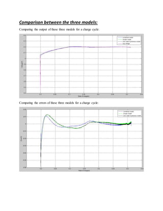
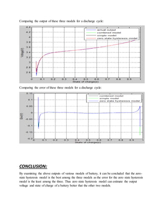
This document summarizes and compares three battery simulation models of increasing complexity: a model with only state of charge (SOC) as a state, a combined model that estimates voltage as a function of SOC and current, and a zero-state hysteresis model. The zero-state hysteresis model accounts for hysteresis effects and has the lowest error compared to the test data, making it the best model. All models are fitted using a least squares estimation technique and their outputs for charge and discharge cycles are analyzed and compared.

1. BATTERY MODEL
SIMULATION
Swayambhu Nath Ray
BEE-IV-B2, JADAVPURUNIVERSITY

2. Introduction:
This report includes simulation of three types of battery models in Matlab, starting from simple
parameters with increasing number of parameters to make our estimation better. Least square
estimation technique is used for this purpose.
Cells:
An electric battery is a device consisting of one or more electrochemical cells that convert stored
chemical energy into electrical energy. Each cell contains a positive terminal, or cathode, and a
negative terminal, or anode. Electrolytes allow ions to move between the electrodes and
terminals, which allows current to flow out of the battery to perform work.
State of charge:
The one constant required for the cell model is that, we constrain SOC, denoted by zk, to be a
member of the state vector xk.
The SOC of the cell is the ratio of the remaining capacity to the nominal capacity of the cell,
where the remaining capacity is the number of ampere-hours that can be drawn from the cell at
the C/30 rate before it is fully discharged.
The mathematical expression of SOC:
z(t) = z(0) - ∫
𝑛∗𝑖(𝑡)
𝐶
𝑑𝑡
𝑡
0
Where z(t) is the cell SOC, i(t) is the instantaneous cell current(assumed positive for discharge
and negative for charge), and C is the cell nominal capacity. Cell Coulombic efficiency n = 1 for
discharge and n<=1 for charge.
Using a rectangular approximation for integration and a ‘suitably small’ sampling period dt , a
discrete time approximate recurrence may then be written as
zk+1 = zk -
𝑛∗∆𝑡
𝐶
∗ 𝑖k
This equation is the basic in including SOC in the state vector of the cell model as it is in state
equation format already, with SOC as a state and ik as input. The cell model may be completed
by adding state as necessary, and an output equation.

3. Models with only SOC as a state:
The first three model investigated have state vector xk = zk . That is, the only state in the state
equation is SOC. These models can estimate cell terminal voltage in a limited way, and are
improved upon later using multiple states.
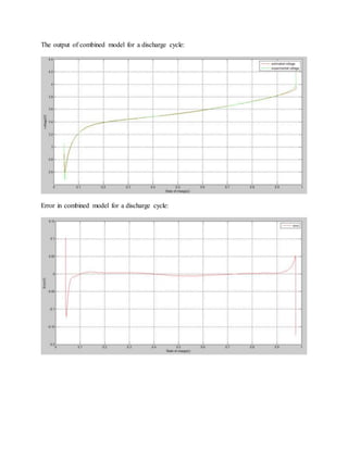
The combined model:
With SOC available as a part of the model state, terminal voltage may be predicted in a number
of different ways.
The state equations describing this model:
zk+1 = zk -
𝑛∗∆𝑡
𝐶
∗ik,
yk = K0 - Rik -
𝐾1
𝑧𝑘
- K2zk + K3ln(zk) + K4ln(1-zk).
The unknown quantities in the combined model may be estimated using a system identification
procedure. This model has the advantage of being “linear in the parameters”; that is, the
unknowns occur linearly in output equation. In order to solve the equations we proceed as
follows:
Y = [y1, y2,….., yN]T
H = [h1, h2, … , hN]T
The rows of H are
hj
T
= [1, ij
+
, ij
-
,
1
𝑧𝑗
, zj, ln(zj), ln(1-zj)] ,
Where ij
+ is equal to ij if ij > 0, ij
- is equal to ij if ij < 0, else ij
+ and ij
- are zero. Then we see that Y
= HƟ where ƟT = [K0, R+, R-, K1, K2, K3, K4] is the vector of unknown parameters. Using the
result from least square estimation technique, Ɵ comes out to be:
Ɵ=(HT
H)-1
HT
Y

4. The output of combined model for a discharge cycle:
Error in combined model for a discharge cycle:

5. The output of combined model for a charge cycle:
Error in combined model for a charge cycle:

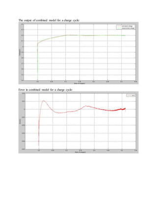
6. The simple model:
With parameter values fit to the “combined model”, we can evaluate its component terms for
further insight. The model output equation may be divided into two additive parts: one part
depending only on SOC and the other depending only on ik:
yk = {K0 -
𝐾1
𝑧𝑘
– K2zk + K3ln(zk) + K4ln(1-zk)} – {Rik}
fn(zk) fn(ik)
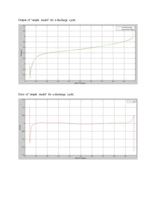
We see that the part of yk that is a function of SOC is attempting to fit the OCV(zk) curve. So, an
easier and more accurate implementation of the combined model is:
zk+1 = zk -
𝑛∗∆𝑡
𝐶
*ik
yk = OCV(zk) - Rik
This model type is also linear in parameters. Offline system identification is done as follows:
Y = [y1 -OCV(z1), y2 - OCV(z2), . . . , yn - OCV(zn)]T
,
H = [h1, h2, . . . , hn]T
.
The rows of H are
hj
T
= [ij
+
, ij
-
].
Again, we see that Y = Hθ, where θT = [R+, R-] is the vector of unknown parameters. We solve
for the parameters θ using the known matrices Y and H as θ = (HTH)-1HTY.

7. Output of ‘simple model’ for a discharge cycle:
Error of ‘simple model’ for a discharge cycle:

8. Output of simple model for a charge cycle:
Error of ‘simple model’ for a charge cycle:
Thus we see that error in simple model is somewhat less than the error in combined model. Thus
simple model is a better estimate than combined model.

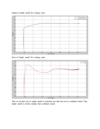
9. The zero-state hysteresis model:
Examination of the previous results exposes some flaws in the models. One subtle effect, which
has serious consequences when predicting SOC, may be seen during rest periods. Following a
discharge, the cell voltage always relaxes to a value less than the true OCV for that SOC, and
following a charge, the cell voltage always relaxes to a value greater than the true OCV. This is
explained by a hysteresis effect occurring in the cell that is not modeled in the combined or
simple models.
A basic model of hysteresis simply adds a term to the output equation:
zk+1 = zk -
𝑛∗∆𝑡
𝐶
*ik
yk = OCV(zk) – skM(zk) - Rik
Where sk represents the sign of the current (with memory during a rest period). For some ƞ
sufficiently small and positive,
1, ik > ƞ
sk = -1, ik< ƞ
sk-1, |ik |<= ƞ
M(zk) is half the difference between the two legs of charge/discharge curve, minus the Rik loss.
This model type is also linear in the parameters. Off-line system identification is done as follows:
Y = [y1 −OCV(z1), y2 − OCV(z2), . . . , yn − OCV(zn)]T
,
and the matrix
H = [h1, h2, . . . , hn]T
.
The rows of H are
hj
T
= [ij
+
, ij
-
, sj].

10. Again, we see that Y = Hθ, where θT = [R+, R-, M] is the vector of unknown parameters. We
solve for the parameters θ using the known matrices Y and H as θ = (HTH)-1HTY.
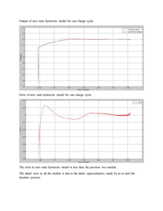
Output of zero state hysteresis model for a discharge cycle:
Error of zero state hysteresis model for one charge cycle:

11. Output of zero state hysteresis model for one charge cycle:
Error of zero state hysteresis model for one charge cycle:
The error in zero state hysteresis model is less than the previous two models.
The initial error in all the models is due to the initial approximation made by us to start the
iteration process.

12. Comparison between the three models:
Comparing the output of these three models for a charge cycle:
Comparing the errors of these three models for a charge cycle:

13. Comparing the output of these three models for a discharge cycle:
Comparing the error of these three models for a discharge cycle:
CONCLUSION:
By examining the above outputs of various models of battery, it can be concluded that the zero-
state hysteresis model is the best among the three models as the error for the zero state hysteresis
model is the least among the three. Thus zero state hysteresis model can estimate the output
voltage and state of charge of a battery better that the other two models.

14. REFERENCES:
 Sungwoo Cho, Hyeonseok Jeong, Chonghun Han, Shanshan Jin, Jae Hwan Lim,
Jeonkeun Oh. State-of-charge estimation for lithium-ion batteries under various operating
conditions using an equivalent circuit model. Journal of Computers and Chemical
Engineering 41(2012) 1-9
 Gregory L. Plett. Extended Kalman Filtering for battery management systems of LiPB-
based HEV battery packs, Part 1. Background . Journal of Power Sources 134(2004) 252-
261
 Gregory L. Plett. Extended Kalman Filtering for battery management systems of LiPB-
based HEV battery packs, Part 2. Modeling and Identification. Journal of Power Sources
134(2004) 262-276
 Gao Xiangyang, Zhang Jun, Ning Ning. Transient Behavior Modeling and Physical
Meaning Analysis for Battery. 2010 International conference on computer application
and system modeling (ICCASM 2010).