SlideShare a Scribd company logo
Research Summary • Brandon McKinzie • Spring 2016
Toy Model Research Summary
Brandon McKinzie
Advisors: Peter Jacobs, Leonardo Milano
I. Introduction
At the Large Hadron Collider (LHC), particles are accelerated in opposing directions at nearly the speed of
light and collide into one another. Due to the enormous amounts of energy involved in such collisions,
thousands of particles are able to be produced. Their properties are detected and analyzed in order to
obtain knowledge about the underlying physics. For example, collisions of heavy nuclei are thought to
produce a state of matter called the quark-gluon plasma (QGP) that existed just microseconds after the Big
Bang. Since the plasma cannot be analyzed directly, we must study the properties of particles that came
from this medium to infer about its properties. Another interesting byproduct of these collisions are very
high-energy groups of particles, collectively called “jets,” that are a consequence of the asymptotic freedom
of QCD; quarks are not allowed to exist unbound (under normal conditions), and so when one is created in
a high-energy collision, many more pairs of quarks are created. This process of fragmentation of the initial
high-energy quark into a cluster of quark/anti-quark pairs and/or triplets results in a jet. Studying the
properties of jets can provide clues about the nature of the QGP, and vice-versa. This relationship is the
source of inspiration for my project.
I will begin by writing a “toy model” of particle collisions that includes the physics of interest and
that results in the production of jets. This will be done exclusively in the C++ programming language
with the aid of the ROOT data analysis framework created at CERN. This part of the analysis is based
on the notion of 2-particle correlations, which says that for certain pairs of particles, their individual
properties have a mutual relationship or connection. Here, this corresponds to selecting a high-energy
particle (the “trigger” hadron) and scanning for the existence of a jet traveling in the opposite direction.
By studying the properties of the resulting jet, depending on what I assign as input parameters, we can
gain an understanding of the interactions involved throughout the collision process. There are, of course,
a few assumptions that underlie this analysis, namely that (1) jets tend to be produced approximately
back-to-back, and that (2) abnormally high energy particles are a good indicator of a jet. The challenge is
reducing the overall signal/noise ratio, where a signal corresponds to correctly identifying a jet, and the
1
noise corresponds to clusters of particles that we erroneously call a jet.
The novelty of this project is in building a model from scratch that relies almost exclusively on sampling
probability distributions from recorded data while also being capable of switching on/off physical process
of interest, such as correlated hadron-jet pairs and the effects of elliptic flow. As of May 13, when this draft
was written, there is still plenty of work to be done, and the project is far from over. This document thus
serves as a summary of what has been done in the past few months with a brief discussion of the next
steps to be taken.
II. Theory
The model relies on a set of commonly used functional forms to describe distributions. Collision events
are simulated via Monte Carlo sampling of measured and/or known probability distributions. The main
particle properties we will be studying are transverse momentum pT, η, and φ. The pseudorapidity,
denoted η, is roughly equivalent to rapidity when pT >> m. It is convenient in that particle production is
approximately uniform over the possible values of η, which are constrained by detector geometry, since
η ≡ −ln tan
θ
2
(1)
which shows the functional dependence of η on the polar angle θ. The ALICE detector provides good
detection in |η| < 1, and we will restrict our analysis to charged particles at mid-rapidity, |η| < 0.8 to
account for any undesirable fringe effects.
The most naïve approach would assume uniformity in both η and ϕ. However, when two nuclei collide
with a non-zero impact parameter, the spatial overlap in the transverse plane no longer looks spherical, but
can take on an almond shape of the form seen in figure 1 below. This results in a non-uniform density
Figure 1: Schematic picture of elliptic flow in the transverse plane. Source: ref. [5].
2
distribution of particles, also called a spatial anisotropy. Soon thereafter, as the spatial anisotropy lessens, it
is “converted” into a momentum anisotropy among the particles, which allows one to measure the degree
of elliptic flow in each event. Specifically, the predicted number of particles produced at a given value of ϕ
is proportional to a quantity denoted as v2, where
dN
dϕ
∝ 1 + 2v2cos[2(ϕ − ψEP)] (2)
and ψEP represents the angle of the event-plane in ϕ.
Somewhat similarly, the analysis of two-particle correlations is done using distributions of the differences
between two particles’ properties. For example rather than plotting dN/dϕ of particles, we would plot
dN/d∆ϕ where ∆ϕ is between a specific trigger particle and all others. If any correlations exist, we would
expect to observe a particular structure in such plots for certain regions of the phase space.
There is an observed suppression of hadron production in heavy-ion collisions as compared to indepen-
dent superpositions of nucleon-nucleon collisions. This is expected to be due to energy loss of the partons
as they propagate through the hot and dense QCD medium [1]. To quantify nuclear medium effects at
high pT, the so called nuclear modification factor RAA is used. Defined as ratio of charged particle yield in
Pb-Pb to pp, scaled by number of binary nucleon-nucleon collisions:
RAA(pT) =
(1/NAA
evt )d2NAA
ch /dηdpT
Ncoll (1/N
pp
evt)d2N
pp
ch /dηdpT
(3)
where we use the measured value of Ncoll = 1690 ± 131 for 0 - 5% centrality.
Jet Reconstruction
The two essential stages for any jet algorithm involve (1) identifying the objects belonging to a cluster,
and (2) calculating the kinematic variables that define the jet from the objects defining the cluster [3]. The
clustering algorithm used here, the anti-kT algorithm, relies on the association of measured particles based
on their transverse momentum1
Before defining what is meant by the “anti” in anti-kT, let’s consider the (longitudinally-invariant) kt
algorithm for hadron collider. The algorithm is initialized with a vector of partons from the event, and
each is considered as a proto(or pseudo)-jet. Then, the following distance measures are computed for each
parton/parton pair: (1) dij between all pairs of particles i and j, and (2) diB = p2
ti between every particle i
1This is contrast with clustering done by cone algorithms, which associate particles based on angles relative to a jet axis.
3
and the beam, where
dij = min(p2
ti, p2
tj)
∆R2
ij
R2
(4)
and ∆R2
ij = (yi − yj)2 + (ϕi − ϕj)2 is the distance in (y, ϕ) space between i and j. The parameter R,
informally referred to as the “jet radius,” determines the angular reach of the algorithm [7]. If the minimum
value of these quantities is a diB, then i is designated as a jet; if it is a dij, then i and j are combined into a
single proto-jet by summing their four-vector components. If two particles/objects are merged, they are
replaced in the list by the object resulting from summing their four-vectors [4]. This is repeated until all
proto-jets have become jets. Mathematically, the algorithm terminates when the following evaluates as true:
(!∃i, j)(k2
T,(i,j) < k2
T,i).
The anti-kt jet algorithm uses the distance measures
dij = min(1/p2
ti, 1/p2
tj)
∆R2
ij
R2
(5a)
diB = 1/p2
ti (5b)
, it behaves in some sense like a “perfect” cone algorithm , in that its ard jets are exactly circular on the
y − φ cylinder. We can see that the consequence of inverting all the values (e.g. 1/pT) is that the highest-pT
objects are clustered first.
One way of correcting for background contamination of hard jets involves the use of jet “areas,” which
provide a measure of a given jet’s susceptibility to soft contamination. Jet areas can be determined by
examining the clustering of a large number of additional infinitesimally soft “ghost” particles. Inclusive jets
correspond to all objects that have undergone a “beam” clustering (diB recombination).
III. Particle Generation
Various implementations responsible for generating the particles were explored throughout the course of
the semester. First, an overview will be given of our initial approach, and then a more detailed account will
be given on the current methods employed for particle generation. The first steps were to sample some (as
of yet undetermined) number of particles uniformly within |η| < 1 and 0 < ϕ < 2π. Initially, the model
used the following pT sampling distribution, courtesy of Redmer Alexander Bertens.
P(x) ∝ A(B2
xe−Bx
) + (x > 1)C 0.12 D2 + x2 1 +
1
(0.82)(E)
D2 + x2
−E 1
1 + e− x−F
G
(6)
4
background phi
0 1 2 3 4 5 6
counts
0
2000
4000
6000
8000
10000
background eta
1− 0.5− 0 0.5 1
counts
0
2000
4000
6000
8000
10000
12000
background pt
0 1 2 3 4 5
counts
0
50
100
150
200
250
300
350
400
3
10×
background phi
1− 0.5− 0 0.5 1
backgroundeta
0
1
2
3
4
5
6
Figure 2: Basic distributions for single particles sampled in phi, η, pt, and phi vs. eta.
with the fitting parameters, denoted by capital letters, initialized with the values in table 1. With the help
of the ROOT libraries, this simple implementation alone was able to plot basic particle spectra as seen in
figure ??.
At this stage, such particles were referred to as “background” particles, as they were sampled randomly
from a (generally) soft distribution. Since we are interested in two-particle correlations associated with
jet production, we also designate a single high-pT particle per event as a “trigger” particle, with a
corresponding “associated” particle opposite to it in η and φ. The associated particle’s phi is also Gaussian
smeared, centered at π radians from the trigger with some standard deviation σ ≈ 0.2. The trigger-
associated particle pairs will later serve as what is known as an h+Jet pair. These assumptions are made
from the perspective of two-particle correlations, which stem from the notion that, in the early stages of the
collision, particles can be produced back-to-back with very high momenta.
Next, we incorporate a non-zero v2 parameter, which varies as a function of the given particle’s pT, that
provides information regarding elliptic flow. Specifically, it is known that, in the presence of flow, particles
are not generated uniformly in φ, but rather they exhibit a dependence on v2 in the form,
dN
dφ
∝ 1 + 2v2cos[2(φ − ψEP)] (7)
where ψEP represents the angle of the event-plane in φ. For now, we simplify this by setting ψEP = 0.
A B C D E F G
2.43 ×10⁹ 2.99 1.01 ×10⁷ 0.14 5.6 2.8 0.2
Table 1: Initial values of fit parameters for the first sampling pT distribution used by the model.
5
background phi
0 1 2 3 4 5 6
counts
0
2000
4000
6000
8000
10000
12000
background eta
1− 0.5− 0 0.5 1
counts
0
2000
4000
6000
8000
10000
12000
background pt
0 5 10 15 20 25 30 35
counts
0
50
100
150
200
250
300
350
400
3
10×
background phi
0 1 2 3 4 5 6
backgroundeta
1−
0.5−
0
0.5
1
Figure 3: Trigger particle distributions for φ, η, pT, and η vs. φ.
The resulting change in the background distribution over phi can be seen in figure ??. To be safe, we
assume that v2 can takes on a different value for trigger, associated, and background particles. Having
the ability to alter the v2 parameter for each category also provides us the opportunity to explore how the
event outcomes depend on such a difference. In effect, we have introduced a new independent variable
that we can tune as we please to observe how it affects the physics and/or distributions. A general goal of
the model is to eventually have as many tunable parameters than be switched on/off as the user pleases.
Now that we have the basic phase space information regarding each particle category, we can begin
plotting combinations of these variables. Of particular interest is the difference in phi of the trigger and
associated particle. We expect this distribution to be centered and peaked at ∆φ = π with a roughly
Gaussian spread, since we have essentially defined it as such. For similar reasons, introduction of elliptic
φ∆
0 1 2 3 4 5 6
φ∆dN/d
10000
11000
12000
13000
14000
15000
16000
17000
assoc+bkg
φ-
trig
φ
bkg
φ-
trig
φ
η∆
2− 1.5− 1− 0.5− 0 0.5 1 1.5 2
η∆dN/d
5000
10000
15000
20000
25000
assoc+bkg
η-
trig
η
bkg
η-
trig
η
φ∆
0 1 2 3 4 5 6
η∆
2−
1.5−
1−
0.5−
0
0.5
1
1.5
2
0
50
100
150
200
250
300
350
Figure 4: Plots of ∆φ and ∆η between the trigger particle and all others. The results for background particles are
plotted in red, and the differences for associated particles are plotted in blue. Note that these distributions, collected
in the earliest stages of the project, correspond to events where similar amounts of trigger particles as background
particles were generated, so as to easily examine their different properties.
6
Figure 5: [Source: Figure 2 of ref. [1]]The pT distributions of primary charged particles at mid-rapidity (|h| < 0.8)
in central (0–5%) and peripheral (70–80%) Pb-Pb collisions at
√
sNN = 2.76 TeV. Error bars are statistical only. The
systematic data errors are smaller than the symbols. The scaled pp references are shown as the two curves, the upper
for 0–5% centrality and the lower for 70–80%. The systematic uncertainties of the pp reference spectra are contained
within the thickness of the line.
flow should not greatly alter this shape. However, if we also include differences between the trigger and
background in this distribution, we expect the modulation introduced from a non-zero v2 to show up as a
modulation in the overall ∆φ distribution. We show how v2 affects both (1) the differences between trigger
and all particles and (2) the differences between just trigger and associated particles in figure 4. Since
the trigger itself is more likely to be found in regions along the event-plane, one would expect it to be
more probable that any given be particle be found at nearly the same ϕ or directly opposite from it. The
triangular shape of the δη distribution is what one would expect for differences taken between pairs of
variables all sampled uniformly over [-1, 1] (i.e. it is due to the geometry of our acceptance)
The current implementation relies almost exclusively on sampling from published data to generate
particles and their properties. The pT distribution for the soft background, shown in figure ??, is from
the same ALICE 2010 data we will soon be comparing with [1]. This also provides us a way to check
that our sampling behaves as expected, as we will be able to plot our model’s pT distribution against the
raw data after we apply the appropriate corrections and normalization factors. We now fit the published
pT distribution with a simpler functional form proposed by Hagedorn to describe experimental hadron
7
Figure 6: A CMS event containing a leading and subleading jet, indicated in red. Credit: Alexander Schmah.
production data as a function of pT over a wide range [6].
E
d3σ
d3 p
= C 1 +
pT
p0
−n
(8)
Although simple in appearance, this function proved to fit the distributions quite well.2
IV. Jet Finder
Now that we can properly generate basic events with high-multiplicity and particles exhibiting elliptic flow,
we can begin searching for the existence of jets. The easiest way to begin this task is to artificially embed a
jet in a known location in the eta-phi phase space and tell our jet finder to search for it; if it reports finding
our embedded jet, and our embedded jet only, we have succeeded in writing an elementary jet finder. From
there, we will improve it so that it can handle more realistic (and much more challenging) events.
After embedding a jet in our simulation over the background, we should expect to see something
like Figure 6 upon plotting eta vs. phi. Any competent jet finder ought to be able to select the particles
displayed in red, which can be distinguished by their abnormally high transverse energy. Although finding
such outliers may seem like a straightforward task, we are seldom presented with the clean-cut distinctions
seen in figure 6. More often, we will be tasked with determining which clusters of particles in a sea of
possibly thousands of background tracks were produced by a hard scattering process.
2One unintended but amusing result was discovered upon plotting the ratio of our model over the reconstructed AOD data that
deviated significantly from unity. It turned out that our model was sampling from the scaled pp reference in figure ?? and thus our
ratio was actually RAA(pT); we had verified the published dependence of RAA with pT on accident.
8
jet
T
p
0 10 20 30 40 50 60
T
dp
dN
evtN
1
3−
10
2−
10
1−
10
1
= 2000evtN
R = 0.3, anti-kT
jet
η
0.6− 0.4− 0.2− 0 0.2 0.4 0.6
ηd
dN
evtN
1
0
5
10
15
20
25
30
35
40
= 2000evtN
R = 0.3, anti-kT
jet
ϕ
0 1 2 3 4 5 6
ϕd
dN
evtN
1
0
1
2
3
4
5
6
7
= 2000evtN
R = 0.3, anti-kT
Figure 7: Basic jet quantities corresponding to the simplest simulation settings. Specifically, these correspond to 2000
generated events, each with (fixed) track multiplicity of 16673. Tracks have sampled distributions like those seen in
figure 2. Track acceptance is restricted to |η| < 0.9. No minimum value of jet pT, typically denoted as pT,min, is passed
to FastJet.
The toy model both generates the events as well as analyzing them with the help of the FastJet
framework. The particles are clustered using the anti-kT algorithm with a default value of R = 0.3 unless
stated otherwise (we will soon explore how varying R can alter results). The clustering returns a vector
of PseudoJet objects, which represent the proto-jets discussed earlier in the Theory section. To begin we
explore various scenarios/checks on the jet finder to ensure quality performance. For now, we analyze the
case of model particle generation with (a) v2 set to 0, (b) track multiplicity constant for all events, and (c)
a 100% tracking efficiency (i.e. all simulated particles are successfully “detected”). This is important for
developing a baseline reference before incorporating the more complex model parameters.
The simplest results are shown in figure 7 with all relevant details regarding how the events were
generated addressed in the caption. It is important to note that, since no transverse momentum cut is
applied to the accepted jets, the number of jets found in the events are not infrared safe quantities [7].
For now, this cut (which is typically included) is omitted because it will be useful for estimating the soft
background/underlying event.
Although the pT and ϕ distributions match expectations4, η will prove to exhibit unanticipated behavior
throughout the remainder of this report. For this reason, we will scrutinize it in greater detail as an attempt
to discover the root cause of its shape. In theory, we would expect the jet η distribution to be flat, as is the
case for the single-particle tracks; there is no reason a priori that jets should be detected preferentially in
certain regions of η but not others. The most likely explanation, and the explanation that I will make a case
for throughout the report, is that the strange shape is ultimately a geometrical consequence of clustering
3This value is the measured charged particle multiplicity for collision centralities of 2.5% from ALICE data in reference [1].
4Given that no cuts have been applied at this stage.
9
Jet Aea
0 0.020.040.060.08 0.10.120.140.160.18 0.2
η
0.8−
0.6−
0.4−
0.2−
0
0.2
0.4
0.6
0.8
0
100
200
300
400
500
Jet Aea
0 0.05 0.1 0.15 0.2 0.25 0.3 0.35 0.4
η
0.6−
0.4−
0.2−
0
0.2
0.4
0.6
0
50
100
150
200
250
300
350
Jet Aea
0
0.1
0.2
0.3
0.4
0.5
0.6η
0.4−
0.2−
0
0.2
0.4
0
20
40
60
80
100
120
140
160
180
200
Jet Aea
0
0.2
0.4
0.6
0.8
1
η
0.4−
0.3−
0.2−
0.1−
0
0.1
0.2
0.3
0.4
0
20
40
60
80
100
120
140
160
180
200
220
240
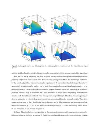
Figure 8: Surface plots of jet η and A for (top-left) R = 0.2, (top-right) R = 0.3, (lower-left) R = 0.4, and (lower-right)
R = 0.5.
with the anti-kT algorithm restricted to a region of η comparable to R, the angular reach of the algorithm.
First, we can see by inspecting the plots in figure 8 that distributions in η deviate from expectations
primarily for jets with areas close to zero. This is a direct consequence of how the clustering is performed
by the anti-kT algorithm. Upon reviewing the equations in 5, we see that the clustering will evolve by
sequentially grouping nearby high-pT tracks until their associated proto-jet has a large enough pT to be
designated as a jet. Near the end of the clustering process, however, there will inevitably be small-area
proto-jets scattered in (η, ϕ) that either don’t meet the criteria to merge with a neighboring proto-jet or are
situated such that all tracks within R have already been assigned to a jet. Therefore, it is unsurprising to
observe uniformity in η for the large-area jets and less conventional behavior for small-are jets. There does
appear to be a trend in the η distribution for the low-area jets as R increases that is a consequence of the
boundary condition |ηtrk| < 0.9. If our acceptance was larger, say |η| < 2.0, such boundary effects would
be less noticeable, as can be seen in figure 9.
In figure 11a, distributions corresponding to the number of reconstructed jets per event are shown for
different values of the input jet radius, R. Again, the number of jets depends on the clustering process
10
Jet Area
0 0.02 0.04 0.06 0.08 0.1 0.12 0.14 0.16 0.18
η
2−
1.5−
1−
0.5−
0
0.5
1
1.5
2
0
20
40
60
80
100
120
Jet Area
0 0.05 0.1 0.15 0.2
0.25 0.3 0.35 0.4
η
2−
1.5−
1−
0.5−
0
0.5
1
1.5
2
0
10
20
30
40
50
60
70
Jet Area
0
0.1
0.2
0.3
0.4
0.5
0.6
0.7
η
1.5−
1−
0.5−
0
0.5
1
1.5
0
5
10
15
20
25
30
35
40
45
Jet Area
0
0.2
0.4
0.6
0.8
1
η
1.5−
1−
0.5−
0
0.5
1
1.5
0
5
10
15
20
25
30
35
Figure 9: Jet area and η distributions with an increased acceptance of |η| < 2.0. All plots correspond to model
simulations of 200 events with (top-left) R = 0.2, (top-right) R = 0.3, (lower-left) R = 0.4, and (lower-right) R = 0.5.
performed by the anti-kT algorithm. The distributions take the form of univariate Gaussians, as opposed to
delta functions, due to the usual variability exhibited in Monte-Carlo sampling methods.
As the value of R increases, the number of measured jets per event decreases. This is nothing more than
a consequence of geometry, since R determines the angular reach of the anti-kT algorithm in η − ϕ space.
Therefore, since no two reconstructed jets can overlap in η − ϕ, we have that large R corresponds to less
reconstructed jets per event. These geometrical/boundary-condition effects will be evident in many of the
plots that follow, such as in figure 11b.
Henceforth, a cut is applied required A > a(R), where the value of the minimum threshold, a(R),
depends on the value of R. They are determined, for a given value of R, by visually inspecting the jet
area distribution for the local minimum between the two outer peaks. This cut serves to further reduce
background, as can be seen in the right-hand side plot of figure 12. It is clear that rejecting the jets with low
area results in a lower proportion of jet candidates with pT = ρA. This can be understood when considering
that lower-area jets are reconstructed near the end of the clustering algorithm, when the highest-pT tracks
have already been clustered and the number of tracks within the algorithm’s angular reach has decreased.
Since we are seeking real jets resulting from hard processes, we reject the low-area jets due to their high
probability of consisting of background particles. The resulting background-subtracted pT distributions for
11
T
p
0 20 40 60 80 100 120 140
T
dp
dN
evtN
1
3−
10
2−
10
1−
10
1
R = 0.2; A > 0.13
R = 0.3; A > 0.28
R = 0.4; A > 0.50
R = 0.5; A > 0.79
nEvents: 2000
| < 0.9track
η|
η
0.8− 0.6− 0.4− 0.2− 0 0.2 0.4 0.6 0.8
ηd
dN
evtN
1
0
10
20
30
40
50
R = 0.2; A > 0.13
R = 0.3; A > 0.28
R = 0.4; A > 0.50
R = 0.5; A > 0.79
Num Events: 2000
ϕ
0 1 2 3 4 5 6
ϕd
dN
evtN
1
0
2
4
6
8
10
R = 0.2; A > 0.13
R = 0.3; A > 0.28
R = 0.4; A > 0.50
R = 0.5; A > 0.79
Num Events: 2000
(a) (Left to right) Distributions for jet pT, η, and ϕ.
T
p
0 10 20 30 40 50 60 70 80
T
dp
dN
evtN
1
2−
10
1−
10
1
10
R = 0.2; A > 0.13
R = 0.3; A > 0.28
R = 0.4; A > 0.50
R = 0.5; A > 0.79
nEvents: 200
| < 2.0track
η|
η
2− 1.5− 1− 0.5− 0 0.5 1 1.5 2
ηd
dN
evtN
1
0
5
10
15
20
25
30
35
40
45
R = 0.2; A > 0.13
R = 0.3; A > 0.28
R = 0.4; A > 0.50
R = 0.5; A > 0.79
Num Events: 200
ϕ
0 1 2 3 4 5 6
ϕd
dN
evtN
1
0
5
10
15
20
25
30
R = 0.2; A > 0.13
R = 0.3; A > 0.28
R = 0.4; A > 0.50
R = 0.5; A > 0.79
Num Events: 200
(b) (Left to right) Distributions for jet pT, η, and ϕ.
Figure 10: 10a shows distributions, each for various values of R, using the same parameters |η| < 0.9 and Nevt = 2000.
10b shows the result of increasing to |η| < 2.0.
different values of R are shown in figure 13.
As R increases, the width of distribution increases, meaning an increased proportion of jets with pT
significantly different than the estimated background. Notice that as R approaches zero, the distributions
should tend toward those of the single-particle tracks.
12
Num Jets per Event
20 40 60 80 100 120
Counts
0
100
200
300
400
500
600
R = 0.2; A > 0.13
R = 0.3; A > 0.28
R = 0.4; A > 0.50
R = 0.5; A > 0.79
nEvents: 2000
| < 0.9track
η|
(a) The number of jets per event reconstructed by FastJet,
shown for different input values of R.
Jet Area
0 0.2 0.4 0.6 0.8 1
dA
dN
evtN
1
1−
10
1
10
2
10
3
10
2
(0.2)π
2
(0.3)π
2
(0.4)π
2
(0.5)π
R = 0.2; A > 0.13
R = 0.3; A > 0.28
R = 0.4; A > 0.50
R = 0.5; A > 0.79
nEvents: 2000
| < 0.9track
η|
(b) The event-normalized distributions of reconstructed
jet areas for different values of R. The dashed vertical
lines indicate where Jet Area = πR2 for each value of R.
Figure 11: Illustration of how jet quantities can vary with R. (a) Number of reconstructed jets per event. (b) Distribution
of reconstructed jet areas.
Area
0 0.05 0.1 0.15 0.2 0.25 0.3 0.35 0.4 0.45 0.5
Counts
0
200
400
600
800
1000
1200
1400
1600
1800
2000
2200
2400 R = 0.3, anti-kT
A > 0.15
= 0.5
T
p
No. Events: 1000
Below Acceptance
Within Acceptance
Aρ-jet,reco
T
p
20− 0 20 40 60 80
Counts
1
10
2
10
3
10
4
10 R = 0.3, anti-kT
A > 0.15
= 0.5
T
p
No. Events: 1000
Without Area Cut
With Area Cut
Figure 12: Illustration of how the jet area cut can affect pT distribution for R = 0.3. Left: An area cut requiring A >
0.15 is applied. Blue represents the region that is kept, while green represents the region rejected. Right: background-
subtracted jet pT distribution shown for jets that passed that area cut (blue), as well as all jets where no area cut was
applied (green).
V. Incorporating Data
We use raw ALICE AOD data from (insert year here) that needs to be corrected for non-perfect detector
efficiency ε. The specific efficiency we are concerned with here is ε = Nreco
Ngen
, which is the fraction of particles
13
Aρ-
T
p
30− 20− 10− 0 10 20 30 40
T
dp
dN
evtN
1
3−
10
2−
10
1−
10
1
10
R = 0.2; A > 0.13
R = 0.3; A > 0.28
R = 0.4; A > 0.50
R = 0.5; A > 0.79
nEvents: 2000
| < 0.9track
η|
Figure 13: Illustration of how the jet area cut can affect pT distribution for R = 0.3. Left: An area cut requiring A >
0.15 is applied. Blue represents the region that is kept, while green represents the region rejected. Right: background-
subtracted jet pT distribution shown for jets that passed that area cut (blue), as well as all jets where no area cut was
applied (green).
that were reconstructed (i.e. found in the data) out of the number actually generated in the collision. This
is required because not all particles created during the collision are perfectly reconstructed/detected at
all. Since we are aware of this shortcoming, we apply 1/ε to the data so as to obtain the true distribu-
tions/numbers of particles corresponding to physical reality. Luckily, this process is so common that results
from Monte Carlo simulations for specific datasets are readily available that provide the user with efficiency
values as a function of particle variables. In particular, we apply this 1ε weight to each track, given the
value of the track’s pt and η as well as the event centrality and the primary collision z-vertex. Another
approach, as seen in figure 14 is leaving the AOD data the same (after applying normalization factors)
and instead applying ε to the model. What this means conceptually is comparing the data, which contains
missing tracks lost due to the detector efficiency, with a version of the model wherein generated particles
have some probability ε of not being recorded. Note that ε here is still a function of the particle properties
in phase space, so this probability changes as the model considers new particles. The main takeaway from
figure 14 is the excellent agreement between the published ALICE data and the reconstructed AOD data.
The model (blue) sits above the rest due to normalization issues. Specifically, the model could only sample
particle multiplicities starting at 2.5% centrality, since that was the lowest data point available.
Since this discrepancy was a valid physical result, new methods were needed to align the model properly
with observed data. One approach was only comparing with data points above pT = 0.5 and modifying
14
the model to generate events with charged-particle multiplicities given by
(1.8)(2.0 ∗ π)
Nevt
20.
0.5
1
2.πpT
d2N
dηdpT
dpT (9)
However, one sees that there is a factor of 1
pT
“embedded” within the data we sample from, and it doesn’t
appear that there is any clean way of removing this pT dependent factor. The reason it is important to get
the charged multiplicity value correct, on average, over events is because it directly impacts both (1) the
histogram magnitudes after normalizations and (more importantly) (2) it effects the simulated efficiencies
given by ε. Although it was rather trivial to apply 1/ε to the AOD data, the reverse method of applying ε
(GeV/c)T
p
0 2 4 6 8 10 12 14 16 18 20
-2
(GeV/c)
ηdT
dp
ch
N2
d
T
pπ2
1
evtN
1
5−
10
4−
10
3−
10
2−
10
1−
10
1
10
2
10
3
10
Toy Model
ALICE (Data)
ALICE (Paper)
CMS (Paper)
(GeV/c)
T
p
2 4 6 8 10 12 14 16 18 20
RatioT
p
0
0.2
0.4
0.6
0.8
1
1.2
ALICE (Data) / ALICE (Paper)
Figure 14: Comparisons between model and various forms of data. Now, we apply the inefficiency to the model instead
of 1/ε to the raw AOD data.
15
to the model remains a problem.
VI. What’s Next
There are three major steps needed to complete this stage of the project.
1. Successfully simulate events with multiplicities given by Ngen · ε where Ngen represents the multiplicity
sampled as a function of centrality for fully corrected/published data. If the model can reproduce the
same distributions as data, including this new addition of accounting for detector inefficiencies, it can
be used to generalize for other detectors (given their efficiencies).
2. Implement h+Jet events in Pythia and merge them into the current model of the soft combinatorial
background. The fastjet implementation is already in place and ready; all that is needed is a more
complicated technique for introducing the jets themselves.
3. Subtracting out the background in the pT distributions by an amount δpT = p
jet,reco
T − pembed
T − ρA,
where ρ is the background momentum density in η − φ space and A is the area of a jet cone given by
the inputs to fastjet.
VII. Conclusion
Although the project is far from over, this draft has explored some of our approaches for building a reliable
toy model that is capable of generalizing well to new sets of data. Decisions are still being made with
regards to the details of implementation, but the vast majority of the code base is in place and easy to modify.
At present, the model consists of an EventGenerator to determine what high-level physical processes will
occur (e.g. triggering and v2 switches), a JetFinder designed to interface well with the EventGenerator and
cluster on likely regions with jets, and many helpers that serve to make the jobs of EventGenerator and
JetFinder as simple/abstracted as possible (e.g. an EventFunctions helper that takes care of the details of
sampling/fitting/etc so the EventGenerator can focus solely on high-level event decisions). The next steps,
as outlined in the previous section, are clear and in the process of being completed. Overall, the experience
of building a model of ultrarelativistic collisions from scratch to where it is now has been rewarding and
educational. I am incredibly grateful to Leonardo Milano, Peter Jacobs, and many other members of the
ALICE collaboration for guiding me throughout this process and teaching me the seemingly countless
subtleties involved in an experimental analysis.
16
References
[1] ALICE Collaboration. Suppression of Charged Particle Production at Large Transverse Momentum in
Central Pb-Pb Collisions at
√
sNN = 2.76 TeV. arXiv:1012.1004v1 (nucl-ex), 2010.
[2] Alexander Schmah. Jet Production in Au+Au Collisions at STAR. Presentation.
[3] J. M. Campbell, J. W. Huston and W. J. Stirling, Rept. Prog. Phys. 70, 89 (2007). [arXiv:hep-ph/0611148]
[4] S. Ellis, et al. Jets in Hadron-Hadron Collisions. (2007). arXiv:0712.2447.
[5] Ullrich Heinz. Concepts in Heavy-Ion Physics. Department of Physics, The Ohio State University, Colum-
bus, OH 43210, USA.
[6] C. Wong and G. Wilk. Tsallis Fits to pT Spectra and Multiple Hard Scattering in pp Collisions at LHC.
arXiv:1305.2627
[7] M. Cacciari et al., “Fastjet user manual”
17
VIII. Appendix
A. Emphasizing Quality Code
Overall, simplicity and ease of use was a primary goal in developing the codebase for this model. The
model obeys the object-oriented paradigm and strives to use classes and methods with intuitive names and
behavior. For example, by using the libraries that I’ve written, the following code is all that is needed to
generate a single event and run the jet finder on the produced particles. Managing complexity and writing
modular code is especially crucial when designing a model that may require new components to be built in
some unknown order in the future.
Figure 15: Screenshot taken of the innermost loop of the toy model interface. The user can both control event selection
and query the objects for desired event information. A static Printer class, tailored to accept various outputs of the
model classes, is available for quickly examining outputs and debugging.
B. More Figures
18
(GeV/c)
T
p
0 20 40 60 80 100 120 140 160
T
dp
dN
T
pπ2
1
7−
10
6−
10
5−
10
4−
10
3−
10
2−
10
1−
10
1
10
2
10
η
1− 0.8− 0.6− 0.4− 0.2− 0 0.2 0.4 0.6 0.8 1
ηd
dN
0
200
400
600
800
1000
1200
1400
1600
1800
2000
3
10×
φ
0 1 2 3 4 5 6
φd
dN
1340
1350
1360
1370
1380
1390
3
10×
(GeV/c)
T
p
0 20 40 60 80 100 120 140 160
T
dp
dN
T
pπ2
1
ε
1
7−
10
6−
10
5−
10
4−
10
3−
10
2−
10
1−
10
1
10
2
10
η
1− 0.8− 0.6− 0.4− 0.2− 0 0.2 0.4 0.6 0.8 1
ηd
dN
ε
1
0
200
400
600
800
1000
1200
1400
1600
1800
2000
2200
3
10×
φ
0 1 2 3 4 5 6
φd
dN
ε
1
1530
1540
1550
1560
1570
1580
1590
3
10×
(GeV/c)
T
p
0 2 4 6 8 10 12 14 16 18 20
T
dp
dN
T
pπ2
1
7−
10
6−
10
5−
10
4−
10
3−
10
2−
10
1−
10
η
1− 0.8− 0.6− 0.4− 0.2− 0 0.2 0.4 0.6 0.8 1
ηdN/d
4000
5000
6000
7000
8000
9000
10000
11000
φ
0 1 2 3 4 5 6
φdN/d
4000
5000
6000
7000
8000
9000
10000
Figure 16: Comparison of pT distributions from reconstructed ALICE data, published ALICE data, published CMS
data, and the toy model (which samples from the published ALICE data). Discrepancies are due to how multiplicity
was obtained at this stage (almost fixed now) since only had access to 2.5% centrality and above. Also, min pT cutoff
may play a role.
19
η
1− 0.8− 0.6− 0.4− 0.2− 0 0.2 0.4 0.6 0.8 1
ε1/
0
200
400
600
800
1000
1200
1400
(GeV/c)
T
p
2 4 6 8 10 12 14
ε1/
1020
1030
1040
1050
1060
1070
1080
1090
centrality
0 20 40 60 80 100
ε1/
5200
5220
5240
5260
5280
5300
5320
5340
5360
5380
z-vtx (cm)
10− 8− 6− 4− 2− 0 2 4 6 8 10
ε1/
2640
2645
2650
2655
2660
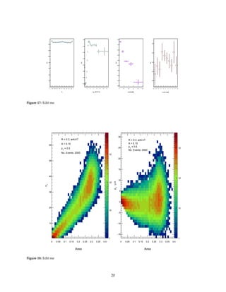
Figure 17: Edit me.
Area
0 0.05 0.1 0.15 0.2 0.25 0.3 0.35 0.4
T
p
10
20
30
40
50
60
1
10
2
10
3
10
R = 0.3, anti-kT
A > 0.15
= 0.5
T
p
No. Events: 2000
Area
0 0.05 0.1 0.15 0.2 0.25 0.3 0.35 0.4
Aρ-
T
p
15−
10−
5−
0
5
10
15
20
25
30
1
10
2
10
3
10
R = 0.3, anti-kT
A > 0.15
= 0.5
T
p
No. Events: 2000
Figure 18: Edit me
20
ρ
106 108 110 112 114 116 118 120 122 124 126 128
Counts
0
0.02
0.04
0.06
0.08
0.1
0.12
0.14
0.16
0.18
R = 0.2; A > 0.13
R = 0.3; A > 0.28
R = 0.4; A > 0.50
R = 0.5; A > 0.79
nEvents: 2000
| < 0.9track
η|
η
0.8− 0.6− 0.4− 0.2− 0 0.2 0.4 0.6 0.8
ηd
dN
evtN
1
0
10
20
30
40
50
60
70
80
90
R = 0.2
R = 0.3
R = 0.4
R = 0.5
Num Events: 2000
Jet Area > 0.15
η
0.8− 0.6− 0.4− 0.2− 0 0.2 0.4 0.6 0.8
ηd
dN
evtN
1
0
10
20
30
40
50
60
70
80
90
R = 0.2
R = 0.3
R = 0.4
R = 0.5
Num Events: 2000
Jet Area > 0.15
21
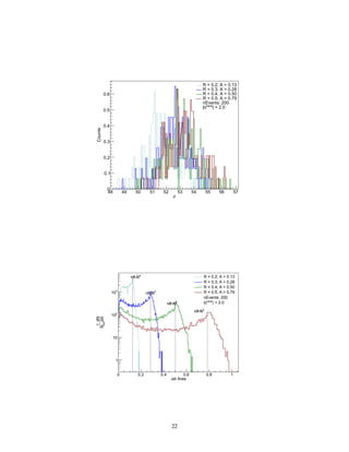
ρ
48 49 50 51 52 53 54 55 56 57
Counts
0
0.1
0.2
0.3
0.4
0.5
0.6
R = 0.2; A > 0.13
R = 0.3; A > 0.28
R = 0.4; A > 0.50
R = 0.5; A > 0.79
nEvents: 200
| < 2.0track
η|
Jet Area
0 0.2 0.4 0.6 0.8 1
dA
dN
evtN
1
1
10
2
10
3
10
2
(0.2)π
2
(0.3)π
2
(0.4)π
2
(0.5)π
R = 0.2; A > 0.13
R = 0.3; A > 0.28
R = 0.4; A > 0.50
R = 0.5; A > 0.79
nEvents: 200
| < 2.0track
η|
22
Num Jets per Event
50 100 150 200 250
Counts
0
10
20
30
40
50
R = 0.2; A > 0.13
R = 0.3; A > 0.28
R = 0.4; A > 0.50
R = 0.5; A > 0.79
nEvents: 200
| < 2.0track
η|
Aρ-
T
p
20− 10− 0 10 20 30
T
dp
dN
evt
N
1
2−
10
1−
10
1
10
R = 0.2; A > 0.13
R = 0.3; A > 0.28
R = 0.4; A > 0.50
R = 0.5; A > 0.79
nEvents: 200
| < 2.0track
η|
23

More Related Content

What's hot

Dft presentation
Dft presentationDft presentation
Dft presentation
Saibalendu Sarkar
 
BNL_Research_Poster
BNL_Research_PosterBNL_Research_Poster
BNL_Research_Poster
Brandon McKinzie
 
UNF Undergrad Physics
UNF Undergrad PhysicsUNF Undergrad Physics
UNF Undergrad Physics
Nick Kypreos
 
Ab initio md
Ab initio mdAb initio md
Ab initio md
yudhaarman
 
Lab4 slides
Lab4 slidesLab4 slides
Lab4 slides
Heather Kulik
 
Electron wave function of first 3 states
Electron wave function of first 3 statesElectron wave function of first 3 states
Electron wave function of first 3 states
vijayakumar sivaji
 
NANO266 - Lecture 6 - Molecule Properties from Quantum Mechanical Modeling
NANO266 - Lecture 6 - Molecule Properties from Quantum Mechanical ModelingNANO266 - Lecture 6 - Molecule Properties from Quantum Mechanical Modeling
NANO266 - Lecture 6 - Molecule Properties from Quantum Mechanical Modeling
University of California, San Diego
 
Part VIII - The Standard Model
Part VIII - The Standard ModelPart VIII - The Standard Model
Part VIII - The Standard Model
Maurice R. TREMBLAY
 
Introduction to Electron Correlation
Introduction to Electron CorrelationIntroduction to Electron Correlation
Introduction to Electron Correlation
Albert DeFusco
 
A new approach to the higgs field
A new approach to the higgs fieldA new approach to the higgs field
A new approach to the higgs field
Eran Sinbar
 
DOI: 10.1007/s10773-009-0027-9
DOI: 10.1007/s10773-009-0027-9DOI: 10.1007/s10773-009-0027-9
DOI: 10.1007/s10773-009-0027-9
1neviv0
 
Basics of DFT+U
Basics of DFT+U Basics of DFT+U
Basics of DFT+U
Burak Himmetoglu
 
NANO266 - Lecture 3 - Beyond the Hartree-Fock Approximation
NANO266 - Lecture 3 - Beyond the Hartree-Fock ApproximationNANO266 - Lecture 3 - Beyond the Hartree-Fock Approximation
NANO266 - Lecture 3 - Beyond the Hartree-Fock Approximation
University of California, San Diego
 
Hadronic1z 1
Hadronic1z  1 Hadronic1z  1
Bp219 04-13-2011
Bp219 04-13-2011Bp219 04-13-2011
Bp219 04-13-2011
waddling
 
Molecular Dynamics - review
Molecular Dynamics - review Molecular Dynamics - review
Molecular Dynamics - review
Hamed Hoorijani
 
Black hole entropy leads to the non-local grid dimensions theory
Black hole entropy leads to the non-local grid dimensions theory Black hole entropy leads to the non-local grid dimensions theory
Black hole entropy leads to the non-local grid dimensions theory
Eran Sinbar
 
Webinar about ATK
Webinar about ATKWebinar about ATK
Webinar about ATK
Anders Blom
 
NANO266 - Lecture 7 - QM Modeling of Periodic Structures
NANO266 - Lecture 7 - QM Modeling of Periodic StructuresNANO266 - Lecture 7 - QM Modeling of Periodic Structures
NANO266 - Lecture 7 - QM Modeling of Periodic Structures
University of California, San Diego
 
Uncertainty quantification
Uncertainty quantificationUncertainty quantification
Uncertainty quantification
Anshul Goyal, EIT
 

What's hot (20)

Dft presentation
Dft presentationDft presentation
Dft presentation
 
BNL_Research_Poster
BNL_Research_PosterBNL_Research_Poster
BNL_Research_Poster
 
UNF Undergrad Physics
UNF Undergrad PhysicsUNF Undergrad Physics
UNF Undergrad Physics
 
Ab initio md
Ab initio mdAb initio md
Ab initio md
 
Lab4 slides
Lab4 slidesLab4 slides
Lab4 slides
 
Electron wave function of first 3 states
Electron wave function of first 3 statesElectron wave function of first 3 states
Electron wave function of first 3 states
 
NANO266 - Lecture 6 - Molecule Properties from Quantum Mechanical Modeling
NANO266 - Lecture 6 - Molecule Properties from Quantum Mechanical ModelingNANO266 - Lecture 6 - Molecule Properties from Quantum Mechanical Modeling
NANO266 - Lecture 6 - Molecule Properties from Quantum Mechanical Modeling
 
Part VIII - The Standard Model
Part VIII - The Standard ModelPart VIII - The Standard Model
Part VIII - The Standard Model
 
Introduction to Electron Correlation
Introduction to Electron CorrelationIntroduction to Electron Correlation
Introduction to Electron Correlation
 
A new approach to the higgs field
A new approach to the higgs fieldA new approach to the higgs field
A new approach to the higgs field
 
DOI: 10.1007/s10773-009-0027-9
DOI: 10.1007/s10773-009-0027-9DOI: 10.1007/s10773-009-0027-9
DOI: 10.1007/s10773-009-0027-9
 
Basics of DFT+U
Basics of DFT+U Basics of DFT+U
Basics of DFT+U
 
NANO266 - Lecture 3 - Beyond the Hartree-Fock Approximation
NANO266 - Lecture 3 - Beyond the Hartree-Fock ApproximationNANO266 - Lecture 3 - Beyond the Hartree-Fock Approximation
NANO266 - Lecture 3 - Beyond the Hartree-Fock Approximation
 
Hadronic1z 1
Hadronic1z  1 Hadronic1z  1
Hadronic1z 1
 
Bp219 04-13-2011
Bp219 04-13-2011Bp219 04-13-2011
Bp219 04-13-2011
 
Molecular Dynamics - review
Molecular Dynamics - review Molecular Dynamics - review
Molecular Dynamics - review
 
Black hole entropy leads to the non-local grid dimensions theory
Black hole entropy leads to the non-local grid dimensions theory Black hole entropy leads to the non-local grid dimensions theory
Black hole entropy leads to the non-local grid dimensions theory
 
Webinar about ATK
Webinar about ATKWebinar about ATK
Webinar about ATK
 
NANO266 - Lecture 7 - QM Modeling of Periodic Structures
NANO266 - Lecture 7 - QM Modeling of Periodic StructuresNANO266 - Lecture 7 - QM Modeling of Periodic Structures
NANO266 - Lecture 7 - QM Modeling of Periodic Structures
 
Uncertainty quantification
Uncertainty quantificationUncertainty quantification
Uncertainty quantification
 

Viewers also liked

Toy Model Overview
Toy Model OverviewToy Model Overview
Toy Model Overview
Brandon McKinzie
 
FinalPoster_MSRP_BrandonMcKinzie
FinalPoster_MSRP_BrandonMcKinzieFinalPoster_MSRP_BrandonMcKinzie
FinalPoster_MSRP_BrandonMcKinzie
Brandon McKinzie
 
SPHENIX Clusterizer Overview
SPHENIX Clusterizer OverviewSPHENIX Clusterizer Overview
SPHENIX Clusterizer Overview
Brandon McKinzie
 
Davis_Research_Report
Davis_Research_ReportDavis_Research_Report
Davis_Research_Report
Brandon McKinzie
 
BNL_Research_Report
BNL_Research_ReportBNL_Research_Report
BNL_Research_Report
Brandon McKinzie
 
EPD_R&D_Proposal
EPD_R&D_ProposalEPD_R&D_Proposal
EPD_R&D_Proposal
Brandon McKinzie
 

Viewers also liked (6)

Toy Model Overview
Toy Model OverviewToy Model Overview
Toy Model Overview
 
FinalPoster_MSRP_BrandonMcKinzie
FinalPoster_MSRP_BrandonMcKinzieFinalPoster_MSRP_BrandonMcKinzie
FinalPoster_MSRP_BrandonMcKinzie
 
SPHENIX Clusterizer Overview
SPHENIX Clusterizer OverviewSPHENIX Clusterizer Overview
SPHENIX Clusterizer Overview
 
Davis_Research_Report
Davis_Research_ReportDavis_Research_Report
Davis_Research_Report
 
BNL_Research_Report
BNL_Research_ReportBNL_Research_Report
BNL_Research_Report
 
EPD_R&D_Proposal
EPD_R&D_ProposalEPD_R&D_Proposal
EPD_R&D_Proposal
 

Similar to Report

Search for microscopic black hole signatures at the large hadron collider
Search for microscopic black hole signatures at the large hadron colliderSearch for microscopic black hole signatures at the large hadron collider
Search for microscopic black hole signatures at the large hadron collider
Sérgio Sacani
 
Bp219 2011
Bp219 2011Bp219 2011
Bp219 2011
waddling
 
Bp219 2011-4.13
Bp219 2011-4.13Bp219 2011-4.13
Bp219 2011-4.13
robertstroud
 
Neutron Skin Measurements at Mainz
Neutron Skin Measurements at MainzNeutron Skin Measurements at Mainz
Neutron Skin Measurements at Mainz
Concettina Sfienti
 
NNBAR SESAPS PRESENTATION FINAL
NNBAR SESAPS PRESENTATION FINALNNBAR SESAPS PRESENTATION FINAL
NNBAR SESAPS PRESENTATION FINAL
Joshua Barrow
 
BP219 class 4 04 2011
BP219 class 4 04 2011BP219 class 4 04 2011
BP219 class 4 04 2011
waddling
 
Ultracold atoms in superlattices as quantum simulators for a spin ordering mo...
Ultracold atoms in superlattices as quantum simulators for a spin ordering mo...Ultracold atoms in superlattices as quantum simulators for a spin ordering mo...
Ultracold atoms in superlattices as quantum simulators for a spin ordering mo...
Alexander Decker
 
Laser Pulsing in Linear Compton Scattering
Laser Pulsing in Linear Compton ScatteringLaser Pulsing in Linear Compton Scattering
Laser Pulsing in Linear Compton Scattering
Todd Hodges
 
Structural, electronic, elastic, optical and thermodynamical properties of zi...
Structural, electronic, elastic, optical and thermodynamical properties of zi...Structural, electronic, elastic, optical and thermodynamical properties of zi...
Structural, electronic, elastic, optical and thermodynamical properties of zi...
Alexander Decker
 
Topology of charge density from pseudopotential density functional theory cal...
Topology of charge density from pseudopotential density functional theory cal...Topology of charge density from pseudopotential density functional theory cal...
Topology of charge density from pseudopotential density functional theory cal...
Alexander Decker
 
Investigation of Steady-State Carrier Distribution in CNT Porins in Neuronal ...
Investigation of Steady-State Carrier Distribution in CNT Porins in Neuronal ...Investigation of Steady-State Carrier Distribution in CNT Porins in Neuronal ...
Investigation of Steady-State Carrier Distribution in CNT Porins in Neuronal ...
Kyle Poe
 
The distribution and_annihilation_of_dark_matter_around_black_holes
The distribution and_annihilation_of_dark_matter_around_black_holesThe distribution and_annihilation_of_dark_matter_around_black_holes
The distribution and_annihilation_of_dark_matter_around_black_holes
Sérgio Sacani
 
SEPnet_Poster-FINAL
SEPnet_Poster-FINALSEPnet_Poster-FINAL
SEPnet_Poster-FINAL
James Blandford
 
MAR_Comprehensive exam on density functional theorypptx
MAR_Comprehensive exam on density functional theorypptxMAR_Comprehensive exam on density functional theorypptx
MAR_Comprehensive exam on density functional theorypptx
MdAbuRayhan16
 
Bands-k-space.pdf
Bands-k-space.pdfBands-k-space.pdf
Bands-k-space.pdf
JoaoVictor699728
 
Elastic scattering reaction of on partial wave scattering matrix, differentia...
Elastic scattering reaction of on partial wave scattering matrix, differentia...Elastic scattering reaction of on partial wave scattering matrix, differentia...
Elastic scattering reaction of on partial wave scattering matrix, differentia...
Alexander Decker
 
On Decreasing of Dimensions of Field-Effect Transistors with Several Sources
On Decreasing of Dimensions of Field-Effect Transistors with Several SourcesOn Decreasing of Dimensions of Field-Effect Transistors with Several Sources
On Decreasing of Dimensions of Field-Effect Transistors with Several Sources
msejjournal
 
punnu-nd-comPresentation2.pptx
punnu-nd-comPresentation2.pptxpunnu-nd-comPresentation2.pptx
punnu-nd-comPresentation2.pptx
SharmilaJayanthi1
 
E27
E27E27
Electron claustrophobia and stability of atoms
Electron claustrophobia and stability of atomsElectron claustrophobia and stability of atoms
Electron claustrophobia and stability of atoms
Maurice Maeck
 

Similar to Report (20)

Search for microscopic black hole signatures at the large hadron collider
Search for microscopic black hole signatures at the large hadron colliderSearch for microscopic black hole signatures at the large hadron collider
Search for microscopic black hole signatures at the large hadron collider
 
Bp219 2011
Bp219 2011Bp219 2011
Bp219 2011
 
Bp219 2011-4.13
Bp219 2011-4.13Bp219 2011-4.13
Bp219 2011-4.13
 
Neutron Skin Measurements at Mainz
Neutron Skin Measurements at MainzNeutron Skin Measurements at Mainz
Neutron Skin Measurements at Mainz
 
NNBAR SESAPS PRESENTATION FINAL
NNBAR SESAPS PRESENTATION FINALNNBAR SESAPS PRESENTATION FINAL
NNBAR SESAPS PRESENTATION FINAL
 
BP219 class 4 04 2011
BP219 class 4 04 2011BP219 class 4 04 2011
BP219 class 4 04 2011
 
Ultracold atoms in superlattices as quantum simulators for a spin ordering mo...
Ultracold atoms in superlattices as quantum simulators for a spin ordering mo...Ultracold atoms in superlattices as quantum simulators for a spin ordering mo...
Ultracold atoms in superlattices as quantum simulators for a spin ordering mo...
 
Laser Pulsing in Linear Compton Scattering
Laser Pulsing in Linear Compton ScatteringLaser Pulsing in Linear Compton Scattering
Laser Pulsing in Linear Compton Scattering
 
Structural, electronic, elastic, optical and thermodynamical properties of zi...
Structural, electronic, elastic, optical and thermodynamical properties of zi...Structural, electronic, elastic, optical and thermodynamical properties of zi...
Structural, electronic, elastic, optical and thermodynamical properties of zi...
 
Topology of charge density from pseudopotential density functional theory cal...
Topology of charge density from pseudopotential density functional theory cal...Topology of charge density from pseudopotential density functional theory cal...
Topology of charge density from pseudopotential density functional theory cal...
 
Investigation of Steady-State Carrier Distribution in CNT Porins in Neuronal ...
Investigation of Steady-State Carrier Distribution in CNT Porins in Neuronal ...Investigation of Steady-State Carrier Distribution in CNT Porins in Neuronal ...
Investigation of Steady-State Carrier Distribution in CNT Porins in Neuronal ...
 
The distribution and_annihilation_of_dark_matter_around_black_holes
The distribution and_annihilation_of_dark_matter_around_black_holesThe distribution and_annihilation_of_dark_matter_around_black_holes
The distribution and_annihilation_of_dark_matter_around_black_holes
 
SEPnet_Poster-FINAL
SEPnet_Poster-FINALSEPnet_Poster-FINAL
SEPnet_Poster-FINAL
 
MAR_Comprehensive exam on density functional theorypptx
MAR_Comprehensive exam on density functional theorypptxMAR_Comprehensive exam on density functional theorypptx
MAR_Comprehensive exam on density functional theorypptx
 
Bands-k-space.pdf
Bands-k-space.pdfBands-k-space.pdf
Bands-k-space.pdf
 
Elastic scattering reaction of on partial wave scattering matrix, differentia...
Elastic scattering reaction of on partial wave scattering matrix, differentia...Elastic scattering reaction of on partial wave scattering matrix, differentia...
Elastic scattering reaction of on partial wave scattering matrix, differentia...
 
On Decreasing of Dimensions of Field-Effect Transistors with Several Sources
On Decreasing of Dimensions of Field-Effect Transistors with Several SourcesOn Decreasing of Dimensions of Field-Effect Transistors with Several Sources
On Decreasing of Dimensions of Field-Effect Transistors with Several Sources
 
punnu-nd-comPresentation2.pptx
punnu-nd-comPresentation2.pptxpunnu-nd-comPresentation2.pptx
punnu-nd-comPresentation2.pptx
 
E27
E27E27
E27
 
Electron claustrophobia and stability of atoms
Electron claustrophobia and stability of atomsElectron claustrophobia and stability of atoms
Electron claustrophobia and stability of atoms
 

Report

  • 1. Research Summary • Brandon McKinzie • Spring 2016 Toy Model Research Summary Brandon McKinzie Advisors: Peter Jacobs, Leonardo Milano I. Introduction At the Large Hadron Collider (LHC), particles are accelerated in opposing directions at nearly the speed of light and collide into one another. Due to the enormous amounts of energy involved in such collisions, thousands of particles are able to be produced. Their properties are detected and analyzed in order to obtain knowledge about the underlying physics. For example, collisions of heavy nuclei are thought to produce a state of matter called the quark-gluon plasma (QGP) that existed just microseconds after the Big Bang. Since the plasma cannot be analyzed directly, we must study the properties of particles that came from this medium to infer about its properties. Another interesting byproduct of these collisions are very high-energy groups of particles, collectively called “jets,” that are a consequence of the asymptotic freedom of QCD; quarks are not allowed to exist unbound (under normal conditions), and so when one is created in a high-energy collision, many more pairs of quarks are created. This process of fragmentation of the initial high-energy quark into a cluster of quark/anti-quark pairs and/or triplets results in a jet. Studying the properties of jets can provide clues about the nature of the QGP, and vice-versa. This relationship is the source of inspiration for my project. I will begin by writing a “toy model” of particle collisions that includes the physics of interest and that results in the production of jets. This will be done exclusively in the C++ programming language with the aid of the ROOT data analysis framework created at CERN. This part of the analysis is based on the notion of 2-particle correlations, which says that for certain pairs of particles, their individual properties have a mutual relationship or connection. Here, this corresponds to selecting a high-energy particle (the “trigger” hadron) and scanning for the existence of a jet traveling in the opposite direction. By studying the properties of the resulting jet, depending on what I assign as input parameters, we can gain an understanding of the interactions involved throughout the collision process. There are, of course, a few assumptions that underlie this analysis, namely that (1) jets tend to be produced approximately back-to-back, and that (2) abnormally high energy particles are a good indicator of a jet. The challenge is reducing the overall signal/noise ratio, where a signal corresponds to correctly identifying a jet, and the 1
  • 2. noise corresponds to clusters of particles that we erroneously call a jet. The novelty of this project is in building a model from scratch that relies almost exclusively on sampling probability distributions from recorded data while also being capable of switching on/off physical process of interest, such as correlated hadron-jet pairs and the effects of elliptic flow. As of May 13, when this draft was written, there is still plenty of work to be done, and the project is far from over. This document thus serves as a summary of what has been done in the past few months with a brief discussion of the next steps to be taken. II. Theory The model relies on a set of commonly used functional forms to describe distributions. Collision events are simulated via Monte Carlo sampling of measured and/or known probability distributions. The main particle properties we will be studying are transverse momentum pT, η, and φ. The pseudorapidity, denoted η, is roughly equivalent to rapidity when pT >> m. It is convenient in that particle production is approximately uniform over the possible values of η, which are constrained by detector geometry, since η ≡ −ln tan θ 2 (1) which shows the functional dependence of η on the polar angle θ. The ALICE detector provides good detection in |η| < 1, and we will restrict our analysis to charged particles at mid-rapidity, |η| < 0.8 to account for any undesirable fringe effects. The most naïve approach would assume uniformity in both η and ϕ. However, when two nuclei collide with a non-zero impact parameter, the spatial overlap in the transverse plane no longer looks spherical, but can take on an almond shape of the form seen in figure 1 below. This results in a non-uniform density Figure 1: Schematic picture of elliptic flow in the transverse plane. Source: ref. [5]. 2
  • 3. distribution of particles, also called a spatial anisotropy. Soon thereafter, as the spatial anisotropy lessens, it is “converted” into a momentum anisotropy among the particles, which allows one to measure the degree of elliptic flow in each event. Specifically, the predicted number of particles produced at a given value of ϕ is proportional to a quantity denoted as v2, where dN dϕ ∝ 1 + 2v2cos[2(ϕ − ψEP)] (2) and ψEP represents the angle of the event-plane in ϕ. Somewhat similarly, the analysis of two-particle correlations is done using distributions of the differences between two particles’ properties. For example rather than plotting dN/dϕ of particles, we would plot dN/d∆ϕ where ∆ϕ is between a specific trigger particle and all others. If any correlations exist, we would expect to observe a particular structure in such plots for certain regions of the phase space. There is an observed suppression of hadron production in heavy-ion collisions as compared to indepen- dent superpositions of nucleon-nucleon collisions. This is expected to be due to energy loss of the partons as they propagate through the hot and dense QCD medium [1]. To quantify nuclear medium effects at high pT, the so called nuclear modification factor RAA is used. Defined as ratio of charged particle yield in Pb-Pb to pp, scaled by number of binary nucleon-nucleon collisions: RAA(pT) = (1/NAA evt )d2NAA ch /dηdpT Ncoll (1/N pp evt)d2N pp ch /dηdpT (3) where we use the measured value of Ncoll = 1690 ± 131 for 0 - 5% centrality. Jet Reconstruction The two essential stages for any jet algorithm involve (1) identifying the objects belonging to a cluster, and (2) calculating the kinematic variables that define the jet from the objects defining the cluster [3]. The clustering algorithm used here, the anti-kT algorithm, relies on the association of measured particles based on their transverse momentum1 Before defining what is meant by the “anti” in anti-kT, let’s consider the (longitudinally-invariant) kt algorithm for hadron collider. The algorithm is initialized with a vector of partons from the event, and each is considered as a proto(or pseudo)-jet. Then, the following distance measures are computed for each parton/parton pair: (1) dij between all pairs of particles i and j, and (2) diB = p2 ti between every particle i 1This is contrast with clustering done by cone algorithms, which associate particles based on angles relative to a jet axis. 3
  • 4. and the beam, where dij = min(p2 ti, p2 tj) ∆R2 ij R2 (4) and ∆R2 ij = (yi − yj)2 + (ϕi − ϕj)2 is the distance in (y, ϕ) space between i and j. The parameter R, informally referred to as the “jet radius,” determines the angular reach of the algorithm [7]. If the minimum value of these quantities is a diB, then i is designated as a jet; if it is a dij, then i and j are combined into a single proto-jet by summing their four-vector components. If two particles/objects are merged, they are replaced in the list by the object resulting from summing their four-vectors [4]. This is repeated until all proto-jets have become jets. Mathematically, the algorithm terminates when the following evaluates as true: (!∃i, j)(k2 T,(i,j) < k2 T,i). The anti-kt jet algorithm uses the distance measures dij = min(1/p2 ti, 1/p2 tj) ∆R2 ij R2 (5a) diB = 1/p2 ti (5b) , it behaves in some sense like a “perfect” cone algorithm , in that its ard jets are exactly circular on the y − φ cylinder. We can see that the consequence of inverting all the values (e.g. 1/pT) is that the highest-pT objects are clustered first. One way of correcting for background contamination of hard jets involves the use of jet “areas,” which provide a measure of a given jet’s susceptibility to soft contamination. Jet areas can be determined by examining the clustering of a large number of additional infinitesimally soft “ghost” particles. Inclusive jets correspond to all objects that have undergone a “beam” clustering (diB recombination). III. Particle Generation Various implementations responsible for generating the particles were explored throughout the course of the semester. First, an overview will be given of our initial approach, and then a more detailed account will be given on the current methods employed for particle generation. The first steps were to sample some (as of yet undetermined) number of particles uniformly within |η| < 1 and 0 < ϕ < 2π. Initially, the model used the following pT sampling distribution, courtesy of Redmer Alexander Bertens. P(x) ∝ A(B2 xe−Bx ) + (x > 1)C 0.12 D2 + x2 1 + 1 (0.82)(E) D2 + x2 −E 1 1 + e− x−F G (6) 4
  • 5. background phi 0 1 2 3 4 5 6 counts 0 2000 4000 6000 8000 10000 background eta 1− 0.5− 0 0.5 1 counts 0 2000 4000 6000 8000 10000 12000 background pt 0 1 2 3 4 5 counts 0 50 100 150 200 250 300 350 400 3 10× background phi 1− 0.5− 0 0.5 1 backgroundeta 0 1 2 3 4 5 6 Figure 2: Basic distributions for single particles sampled in phi, η, pt, and phi vs. eta. with the fitting parameters, denoted by capital letters, initialized with the values in table 1. With the help of the ROOT libraries, this simple implementation alone was able to plot basic particle spectra as seen in figure ??. At this stage, such particles were referred to as “background” particles, as they were sampled randomly from a (generally) soft distribution. Since we are interested in two-particle correlations associated with jet production, we also designate a single high-pT particle per event as a “trigger” particle, with a corresponding “associated” particle opposite to it in η and φ. The associated particle’s phi is also Gaussian smeared, centered at π radians from the trigger with some standard deviation σ ≈ 0.2. The trigger- associated particle pairs will later serve as what is known as an h+Jet pair. These assumptions are made from the perspective of two-particle correlations, which stem from the notion that, in the early stages of the collision, particles can be produced back-to-back with very high momenta. Next, we incorporate a non-zero v2 parameter, which varies as a function of the given particle’s pT, that provides information regarding elliptic flow. Specifically, it is known that, in the presence of flow, particles are not generated uniformly in φ, but rather they exhibit a dependence on v2 in the form, dN dφ ∝ 1 + 2v2cos[2(φ − ψEP)] (7) where ψEP represents the angle of the event-plane in φ. For now, we simplify this by setting ψEP = 0. A B C D E F G 2.43 ×10⁹ 2.99 1.01 ×10⁷ 0.14 5.6 2.8 0.2 Table 1: Initial values of fit parameters for the first sampling pT distribution used by the model. 5
  • 6. background phi 0 1 2 3 4 5 6 counts 0 2000 4000 6000 8000 10000 12000 background eta 1− 0.5− 0 0.5 1 counts 0 2000 4000 6000 8000 10000 12000 background pt 0 5 10 15 20 25 30 35 counts 0 50 100 150 200 250 300 350 400 3 10× background phi 0 1 2 3 4 5 6 backgroundeta 1− 0.5− 0 0.5 1 Figure 3: Trigger particle distributions for φ, η, pT, and η vs. φ. The resulting change in the background distribution over phi can be seen in figure ??. To be safe, we assume that v2 can takes on a different value for trigger, associated, and background particles. Having the ability to alter the v2 parameter for each category also provides us the opportunity to explore how the event outcomes depend on such a difference. In effect, we have introduced a new independent variable that we can tune as we please to observe how it affects the physics and/or distributions. A general goal of the model is to eventually have as many tunable parameters than be switched on/off as the user pleases. Now that we have the basic phase space information regarding each particle category, we can begin plotting combinations of these variables. Of particular interest is the difference in phi of the trigger and associated particle. We expect this distribution to be centered and peaked at ∆φ = π with a roughly Gaussian spread, since we have essentially defined it as such. For similar reasons, introduction of elliptic φ∆ 0 1 2 3 4 5 6 φ∆dN/d 10000 11000 12000 13000 14000 15000 16000 17000 assoc+bkg φ- trig φ bkg φ- trig φ η∆ 2− 1.5− 1− 0.5− 0 0.5 1 1.5 2 η∆dN/d 5000 10000 15000 20000 25000 assoc+bkg η- trig η bkg η- trig η φ∆ 0 1 2 3 4 5 6 η∆ 2− 1.5− 1− 0.5− 0 0.5 1 1.5 2 0 50 100 150 200 250 300 350 Figure 4: Plots of ∆φ and ∆η between the trigger particle and all others. The results for background particles are plotted in red, and the differences for associated particles are plotted in blue. Note that these distributions, collected in the earliest stages of the project, correspond to events where similar amounts of trigger particles as background particles were generated, so as to easily examine their different properties. 6
  • 7. Figure 5: [Source: Figure 2 of ref. [1]]The pT distributions of primary charged particles at mid-rapidity (|h| < 0.8) in central (0–5%) and peripheral (70–80%) Pb-Pb collisions at √ sNN = 2.76 TeV. Error bars are statistical only. The systematic data errors are smaller than the symbols. The scaled pp references are shown as the two curves, the upper for 0–5% centrality and the lower for 70–80%. The systematic uncertainties of the pp reference spectra are contained within the thickness of the line. flow should not greatly alter this shape. However, if we also include differences between the trigger and background in this distribution, we expect the modulation introduced from a non-zero v2 to show up as a modulation in the overall ∆φ distribution. We show how v2 affects both (1) the differences between trigger and all particles and (2) the differences between just trigger and associated particles in figure 4. Since the trigger itself is more likely to be found in regions along the event-plane, one would expect it to be more probable that any given be particle be found at nearly the same ϕ or directly opposite from it. The triangular shape of the δη distribution is what one would expect for differences taken between pairs of variables all sampled uniformly over [-1, 1] (i.e. it is due to the geometry of our acceptance) The current implementation relies almost exclusively on sampling from published data to generate particles and their properties. The pT distribution for the soft background, shown in figure ??, is from the same ALICE 2010 data we will soon be comparing with [1]. This also provides us a way to check that our sampling behaves as expected, as we will be able to plot our model’s pT distribution against the raw data after we apply the appropriate corrections and normalization factors. We now fit the published pT distribution with a simpler functional form proposed by Hagedorn to describe experimental hadron 7
  • 8. Figure 6: A CMS event containing a leading and subleading jet, indicated in red. Credit: Alexander Schmah. production data as a function of pT over a wide range [6]. E d3σ d3 p = C 1 + pT p0 −n (8) Although simple in appearance, this function proved to fit the distributions quite well.2 IV. Jet Finder Now that we can properly generate basic events with high-multiplicity and particles exhibiting elliptic flow, we can begin searching for the existence of jets. The easiest way to begin this task is to artificially embed a jet in a known location in the eta-phi phase space and tell our jet finder to search for it; if it reports finding our embedded jet, and our embedded jet only, we have succeeded in writing an elementary jet finder. From there, we will improve it so that it can handle more realistic (and much more challenging) events. After embedding a jet in our simulation over the background, we should expect to see something like Figure 6 upon plotting eta vs. phi. Any competent jet finder ought to be able to select the particles displayed in red, which can be distinguished by their abnormally high transverse energy. Although finding such outliers may seem like a straightforward task, we are seldom presented with the clean-cut distinctions seen in figure 6. More often, we will be tasked with determining which clusters of particles in a sea of possibly thousands of background tracks were produced by a hard scattering process. 2One unintended but amusing result was discovered upon plotting the ratio of our model over the reconstructed AOD data that deviated significantly from unity. It turned out that our model was sampling from the scaled pp reference in figure ?? and thus our ratio was actually RAA(pT); we had verified the published dependence of RAA with pT on accident. 8
  • 9. jet T p 0 10 20 30 40 50 60 T dp dN evtN 1 3− 10 2− 10 1− 10 1 = 2000evtN R = 0.3, anti-kT jet η 0.6− 0.4− 0.2− 0 0.2 0.4 0.6 ηd dN evtN 1 0 5 10 15 20 25 30 35 40 = 2000evtN R = 0.3, anti-kT jet ϕ 0 1 2 3 4 5 6 ϕd dN evtN 1 0 1 2 3 4 5 6 7 = 2000evtN R = 0.3, anti-kT Figure 7: Basic jet quantities corresponding to the simplest simulation settings. Specifically, these correspond to 2000 generated events, each with (fixed) track multiplicity of 16673. Tracks have sampled distributions like those seen in figure 2. Track acceptance is restricted to |η| < 0.9. No minimum value of jet pT, typically denoted as pT,min, is passed to FastJet. The toy model both generates the events as well as analyzing them with the help of the FastJet framework. The particles are clustered using the anti-kT algorithm with a default value of R = 0.3 unless stated otherwise (we will soon explore how varying R can alter results). The clustering returns a vector of PseudoJet objects, which represent the proto-jets discussed earlier in the Theory section. To begin we explore various scenarios/checks on the jet finder to ensure quality performance. For now, we analyze the case of model particle generation with (a) v2 set to 0, (b) track multiplicity constant for all events, and (c) a 100% tracking efficiency (i.e. all simulated particles are successfully “detected”). This is important for developing a baseline reference before incorporating the more complex model parameters. The simplest results are shown in figure 7 with all relevant details regarding how the events were generated addressed in the caption. It is important to note that, since no transverse momentum cut is applied to the accepted jets, the number of jets found in the events are not infrared safe quantities [7]. For now, this cut (which is typically included) is omitted because it will be useful for estimating the soft background/underlying event. Although the pT and ϕ distributions match expectations4, η will prove to exhibit unanticipated behavior throughout the remainder of this report. For this reason, we will scrutinize it in greater detail as an attempt to discover the root cause of its shape. In theory, we would expect the jet η distribution to be flat, as is the case for the single-particle tracks; there is no reason a priori that jets should be detected preferentially in certain regions of η but not others. The most likely explanation, and the explanation that I will make a case for throughout the report, is that the strange shape is ultimately a geometrical consequence of clustering 3This value is the measured charged particle multiplicity for collision centralities of 2.5% from ALICE data in reference [1]. 4Given that no cuts have been applied at this stage. 9
  • 10. Jet Aea 0 0.020.040.060.08 0.10.120.140.160.18 0.2 η 0.8− 0.6− 0.4− 0.2− 0 0.2 0.4 0.6 0.8 0 100 200 300 400 500 Jet Aea 0 0.05 0.1 0.15 0.2 0.25 0.3 0.35 0.4 η 0.6− 0.4− 0.2− 0 0.2 0.4 0.6 0 50 100 150 200 250 300 350 Jet Aea 0 0.1 0.2 0.3 0.4 0.5 0.6η 0.4− 0.2− 0 0.2 0.4 0 20 40 60 80 100 120 140 160 180 200 Jet Aea 0 0.2 0.4 0.6 0.8 1 η 0.4− 0.3− 0.2− 0.1− 0 0.1 0.2 0.3 0.4 0 20 40 60 80 100 120 140 160 180 200 220 240 Figure 8: Surface plots of jet η and A for (top-left) R = 0.2, (top-right) R = 0.3, (lower-left) R = 0.4, and (lower-right) R = 0.5. with the anti-kT algorithm restricted to a region of η comparable to R, the angular reach of the algorithm. First, we can see by inspecting the plots in figure 8 that distributions in η deviate from expectations primarily for jets with areas close to zero. This is a direct consequence of how the clustering is performed by the anti-kT algorithm. Upon reviewing the equations in 5, we see that the clustering will evolve by sequentially grouping nearby high-pT tracks until their associated proto-jet has a large enough pT to be designated as a jet. Near the end of the clustering process, however, there will inevitably be small-area proto-jets scattered in (η, ϕ) that either don’t meet the criteria to merge with a neighboring proto-jet or are situated such that all tracks within R have already been assigned to a jet. Therefore, it is unsurprising to observe uniformity in η for the large-area jets and less conventional behavior for small-are jets. There does appear to be a trend in the η distribution for the low-area jets as R increases that is a consequence of the boundary condition |ηtrk| < 0.9. If our acceptance was larger, say |η| < 2.0, such boundary effects would be less noticeable, as can be seen in figure 9. In figure 11a, distributions corresponding to the number of reconstructed jets per event are shown for different values of the input jet radius, R. Again, the number of jets depends on the clustering process 10
  • 11. Jet Area 0 0.02 0.04 0.06 0.08 0.1 0.12 0.14 0.16 0.18 η 2− 1.5− 1− 0.5− 0 0.5 1 1.5 2 0 20 40 60 80 100 120 Jet Area 0 0.05 0.1 0.15 0.2 0.25 0.3 0.35 0.4 η 2− 1.5− 1− 0.5− 0 0.5 1 1.5 2 0 10 20 30 40 50 60 70 Jet Area 0 0.1 0.2 0.3 0.4 0.5 0.6 0.7 η 1.5− 1− 0.5− 0 0.5 1 1.5 0 5 10 15 20 25 30 35 40 45 Jet Area 0 0.2 0.4 0.6 0.8 1 η 1.5− 1− 0.5− 0 0.5 1 1.5 0 5 10 15 20 25 30 35 Figure 9: Jet area and η distributions with an increased acceptance of |η| < 2.0. All plots correspond to model simulations of 200 events with (top-left) R = 0.2, (top-right) R = 0.3, (lower-left) R = 0.4, and (lower-right) R = 0.5. performed by the anti-kT algorithm. The distributions take the form of univariate Gaussians, as opposed to delta functions, due to the usual variability exhibited in Monte-Carlo sampling methods. As the value of R increases, the number of measured jets per event decreases. This is nothing more than a consequence of geometry, since R determines the angular reach of the anti-kT algorithm in η − ϕ space. Therefore, since no two reconstructed jets can overlap in η − ϕ, we have that large R corresponds to less reconstructed jets per event. These geometrical/boundary-condition effects will be evident in many of the plots that follow, such as in figure 11b. Henceforth, a cut is applied required A > a(R), where the value of the minimum threshold, a(R), depends on the value of R. They are determined, for a given value of R, by visually inspecting the jet area distribution for the local minimum between the two outer peaks. This cut serves to further reduce background, as can be seen in the right-hand side plot of figure 12. It is clear that rejecting the jets with low area results in a lower proportion of jet candidates with pT = ρA. This can be understood when considering that lower-area jets are reconstructed near the end of the clustering algorithm, when the highest-pT tracks have already been clustered and the number of tracks within the algorithm’s angular reach has decreased. Since we are seeking real jets resulting from hard processes, we reject the low-area jets due to their high probability of consisting of background particles. The resulting background-subtracted pT distributions for 11
  • 12. T p 0 20 40 60 80 100 120 140 T dp dN evtN 1 3− 10 2− 10 1− 10 1 R = 0.2; A > 0.13 R = 0.3; A > 0.28 R = 0.4; A > 0.50 R = 0.5; A > 0.79 nEvents: 2000 | < 0.9track η| η 0.8− 0.6− 0.4− 0.2− 0 0.2 0.4 0.6 0.8 ηd dN evtN 1 0 10 20 30 40 50 R = 0.2; A > 0.13 R = 0.3; A > 0.28 R = 0.4; A > 0.50 R = 0.5; A > 0.79 Num Events: 2000 ϕ 0 1 2 3 4 5 6 ϕd dN evtN 1 0 2 4 6 8 10 R = 0.2; A > 0.13 R = 0.3; A > 0.28 R = 0.4; A > 0.50 R = 0.5; A > 0.79 Num Events: 2000 (a) (Left to right) Distributions for jet pT, η, and ϕ. T p 0 10 20 30 40 50 60 70 80 T dp dN evtN 1 2− 10 1− 10 1 10 R = 0.2; A > 0.13 R = 0.3; A > 0.28 R = 0.4; A > 0.50 R = 0.5; A > 0.79 nEvents: 200 | < 2.0track η| η 2− 1.5− 1− 0.5− 0 0.5 1 1.5 2 ηd dN evtN 1 0 5 10 15 20 25 30 35 40 45 R = 0.2; A > 0.13 R = 0.3; A > 0.28 R = 0.4; A > 0.50 R = 0.5; A > 0.79 Num Events: 200 ϕ 0 1 2 3 4 5 6 ϕd dN evtN 1 0 5 10 15 20 25 30 R = 0.2; A > 0.13 R = 0.3; A > 0.28 R = 0.4; A > 0.50 R = 0.5; A > 0.79 Num Events: 200 (b) (Left to right) Distributions for jet pT, η, and ϕ. Figure 10: 10a shows distributions, each for various values of R, using the same parameters |η| < 0.9 and Nevt = 2000. 10b shows the result of increasing to |η| < 2.0. different values of R are shown in figure 13. As R increases, the width of distribution increases, meaning an increased proportion of jets with pT significantly different than the estimated background. Notice that as R approaches zero, the distributions should tend toward those of the single-particle tracks. 12
  • 13. Num Jets per Event 20 40 60 80 100 120 Counts 0 100 200 300 400 500 600 R = 0.2; A > 0.13 R = 0.3; A > 0.28 R = 0.4; A > 0.50 R = 0.5; A > 0.79 nEvents: 2000 | < 0.9track η| (a) The number of jets per event reconstructed by FastJet, shown for different input values of R. Jet Area 0 0.2 0.4 0.6 0.8 1 dA dN evtN 1 1− 10 1 10 2 10 3 10 2 (0.2)π 2 (0.3)π 2 (0.4)π 2 (0.5)π R = 0.2; A > 0.13 R = 0.3; A > 0.28 R = 0.4; A > 0.50 R = 0.5; A > 0.79 nEvents: 2000 | < 0.9track η| (b) The event-normalized distributions of reconstructed jet areas for different values of R. The dashed vertical lines indicate where Jet Area = πR2 for each value of R. Figure 11: Illustration of how jet quantities can vary with R. (a) Number of reconstructed jets per event. (b) Distribution of reconstructed jet areas. Area 0 0.05 0.1 0.15 0.2 0.25 0.3 0.35 0.4 0.45 0.5 Counts 0 200 400 600 800 1000 1200 1400 1600 1800 2000 2200 2400 R = 0.3, anti-kT A > 0.15 = 0.5 T p No. Events: 1000 Below Acceptance Within Acceptance Aρ-jet,reco T p 20− 0 20 40 60 80 Counts 1 10 2 10 3 10 4 10 R = 0.3, anti-kT A > 0.15 = 0.5 T p No. Events: 1000 Without Area Cut With Area Cut Figure 12: Illustration of how the jet area cut can affect pT distribution for R = 0.3. Left: An area cut requiring A > 0.15 is applied. Blue represents the region that is kept, while green represents the region rejected. Right: background- subtracted jet pT distribution shown for jets that passed that area cut (blue), as well as all jets where no area cut was applied (green). V. Incorporating Data We use raw ALICE AOD data from (insert year here) that needs to be corrected for non-perfect detector efficiency ε. The specific efficiency we are concerned with here is ε = Nreco Ngen , which is the fraction of particles 13
  • 14. Aρ- T p 30− 20− 10− 0 10 20 30 40 T dp dN evtN 1 3− 10 2− 10 1− 10 1 10 R = 0.2; A > 0.13 R = 0.3; A > 0.28 R = 0.4; A > 0.50 R = 0.5; A > 0.79 nEvents: 2000 | < 0.9track η| Figure 13: Illustration of how the jet area cut can affect pT distribution for R = 0.3. Left: An area cut requiring A > 0.15 is applied. Blue represents the region that is kept, while green represents the region rejected. Right: background- subtracted jet pT distribution shown for jets that passed that area cut (blue), as well as all jets where no area cut was applied (green). that were reconstructed (i.e. found in the data) out of the number actually generated in the collision. This is required because not all particles created during the collision are perfectly reconstructed/detected at all. Since we are aware of this shortcoming, we apply 1/ε to the data so as to obtain the true distribu- tions/numbers of particles corresponding to physical reality. Luckily, this process is so common that results from Monte Carlo simulations for specific datasets are readily available that provide the user with efficiency values as a function of particle variables. In particular, we apply this 1ε weight to each track, given the value of the track’s pt and η as well as the event centrality and the primary collision z-vertex. Another approach, as seen in figure 14 is leaving the AOD data the same (after applying normalization factors) and instead applying ε to the model. What this means conceptually is comparing the data, which contains missing tracks lost due to the detector efficiency, with a version of the model wherein generated particles have some probability ε of not being recorded. Note that ε here is still a function of the particle properties in phase space, so this probability changes as the model considers new particles. The main takeaway from figure 14 is the excellent agreement between the published ALICE data and the reconstructed AOD data. The model (blue) sits above the rest due to normalization issues. Specifically, the model could only sample particle multiplicities starting at 2.5% centrality, since that was the lowest data point available. Since this discrepancy was a valid physical result, new methods were needed to align the model properly with observed data. One approach was only comparing with data points above pT = 0.5 and modifying 14
  • 15. the model to generate events with charged-particle multiplicities given by (1.8)(2.0 ∗ π) Nevt 20. 0.5 1 2.πpT d2N dηdpT dpT (9) However, one sees that there is a factor of 1 pT “embedded” within the data we sample from, and it doesn’t appear that there is any clean way of removing this pT dependent factor. The reason it is important to get the charged multiplicity value correct, on average, over events is because it directly impacts both (1) the histogram magnitudes after normalizations and (more importantly) (2) it effects the simulated efficiencies given by ε. Although it was rather trivial to apply 1/ε to the AOD data, the reverse method of applying ε (GeV/c)T p 0 2 4 6 8 10 12 14 16 18 20 -2 (GeV/c) ηdT dp ch N2 d T pπ2 1 evtN 1 5− 10 4− 10 3− 10 2− 10 1− 10 1 10 2 10 3 10 Toy Model ALICE (Data) ALICE (Paper) CMS (Paper) (GeV/c) T p 2 4 6 8 10 12 14 16 18 20 RatioT p 0 0.2 0.4 0.6 0.8 1 1.2 ALICE (Data) / ALICE (Paper) Figure 14: Comparisons between model and various forms of data. Now, we apply the inefficiency to the model instead of 1/ε to the raw AOD data. 15
  • 16. to the model remains a problem. VI. What’s Next There are three major steps needed to complete this stage of the project. 1. Successfully simulate events with multiplicities given by Ngen · ε where Ngen represents the multiplicity sampled as a function of centrality for fully corrected/published data. If the model can reproduce the same distributions as data, including this new addition of accounting for detector inefficiencies, it can be used to generalize for other detectors (given their efficiencies). 2. Implement h+Jet events in Pythia and merge them into the current model of the soft combinatorial background. The fastjet implementation is already in place and ready; all that is needed is a more complicated technique for introducing the jets themselves. 3. Subtracting out the background in the pT distributions by an amount δpT = p jet,reco T − pembed T − ρA, where ρ is the background momentum density in η − φ space and A is the area of a jet cone given by the inputs to fastjet. VII. Conclusion Although the project is far from over, this draft has explored some of our approaches for building a reliable toy model that is capable of generalizing well to new sets of data. Decisions are still being made with regards to the details of implementation, but the vast majority of the code base is in place and easy to modify. At present, the model consists of an EventGenerator to determine what high-level physical processes will occur (e.g. triggering and v2 switches), a JetFinder designed to interface well with the EventGenerator and cluster on likely regions with jets, and many helpers that serve to make the jobs of EventGenerator and JetFinder as simple/abstracted as possible (e.g. an EventFunctions helper that takes care of the details of sampling/fitting/etc so the EventGenerator can focus solely on high-level event decisions). The next steps, as outlined in the previous section, are clear and in the process of being completed. Overall, the experience of building a model of ultrarelativistic collisions from scratch to where it is now has been rewarding and educational. I am incredibly grateful to Leonardo Milano, Peter Jacobs, and many other members of the ALICE collaboration for guiding me throughout this process and teaching me the seemingly countless subtleties involved in an experimental analysis. 16
  • 17. References [1] ALICE Collaboration. Suppression of Charged Particle Production at Large Transverse Momentum in Central Pb-Pb Collisions at √ sNN = 2.76 TeV. arXiv:1012.1004v1 (nucl-ex), 2010. [2] Alexander Schmah. Jet Production in Au+Au Collisions at STAR. Presentation. [3] J. M. Campbell, J. W. Huston and W. J. Stirling, Rept. Prog. Phys. 70, 89 (2007). [arXiv:hep-ph/0611148] [4] S. Ellis, et al. Jets in Hadron-Hadron Collisions. (2007). arXiv:0712.2447. [5] Ullrich Heinz. Concepts in Heavy-Ion Physics. Department of Physics, The Ohio State University, Colum- bus, OH 43210, USA. [6] C. Wong and G. Wilk. Tsallis Fits to pT Spectra and Multiple Hard Scattering in pp Collisions at LHC. arXiv:1305.2627 [7] M. Cacciari et al., “Fastjet user manual” 17
  • 18. VIII. Appendix A. Emphasizing Quality Code Overall, simplicity and ease of use was a primary goal in developing the codebase for this model. The model obeys the object-oriented paradigm and strives to use classes and methods with intuitive names and behavior. For example, by using the libraries that I’ve written, the following code is all that is needed to generate a single event and run the jet finder on the produced particles. Managing complexity and writing modular code is especially crucial when designing a model that may require new components to be built in some unknown order in the future. Figure 15: Screenshot taken of the innermost loop of the toy model interface. The user can both control event selection and query the objects for desired event information. A static Printer class, tailored to accept various outputs of the model classes, is available for quickly examining outputs and debugging. B. More Figures 18
  • 19. (GeV/c) T p 0 20 40 60 80 100 120 140 160 T dp dN T pπ2 1 7− 10 6− 10 5− 10 4− 10 3− 10 2− 10 1− 10 1 10 2 10 η 1− 0.8− 0.6− 0.4− 0.2− 0 0.2 0.4 0.6 0.8 1 ηd dN 0 200 400 600 800 1000 1200 1400 1600 1800 2000 3 10× φ 0 1 2 3 4 5 6 φd dN 1340 1350 1360 1370 1380 1390 3 10× (GeV/c) T p 0 20 40 60 80 100 120 140 160 T dp dN T pπ2 1 ε 1 7− 10 6− 10 5− 10 4− 10 3− 10 2− 10 1− 10 1 10 2 10 η 1− 0.8− 0.6− 0.4− 0.2− 0 0.2 0.4 0.6 0.8 1 ηd dN ε 1 0 200 400 600 800 1000 1200 1400 1600 1800 2000 2200 3 10× φ 0 1 2 3 4 5 6 φd dN ε 1 1530 1540 1550 1560 1570 1580 1590 3 10× (GeV/c) T p 0 2 4 6 8 10 12 14 16 18 20 T dp dN T pπ2 1 7− 10 6− 10 5− 10 4− 10 3− 10 2− 10 1− 10 η 1− 0.8− 0.6− 0.4− 0.2− 0 0.2 0.4 0.6 0.8 1 ηdN/d 4000 5000 6000 7000 8000 9000 10000 11000 φ 0 1 2 3 4 5 6 φdN/d 4000 5000 6000 7000 8000 9000 10000 Figure 16: Comparison of pT distributions from reconstructed ALICE data, published ALICE data, published CMS data, and the toy model (which samples from the published ALICE data). Discrepancies are due to how multiplicity was obtained at this stage (almost fixed now) since only had access to 2.5% centrality and above. Also, min pT cutoff may play a role. 19
  • 20. η 1− 0.8− 0.6− 0.4− 0.2− 0 0.2 0.4 0.6 0.8 1 ε1/ 0 200 400 600 800 1000 1200 1400 (GeV/c) T p 2 4 6 8 10 12 14 ε1/ 1020 1030 1040 1050 1060 1070 1080 1090 centrality 0 20 40 60 80 100 ε1/ 5200 5220 5240 5260 5280 5300 5320 5340 5360 5380 z-vtx (cm) 10− 8− 6− 4− 2− 0 2 4 6 8 10 ε1/ 2640 2645 2650 2655 2660 Figure 17: Edit me. Area 0 0.05 0.1 0.15 0.2 0.25 0.3 0.35 0.4 T p 10 20 30 40 50 60 1 10 2 10 3 10 R = 0.3, anti-kT A > 0.15 = 0.5 T p No. Events: 2000 Area 0 0.05 0.1 0.15 0.2 0.25 0.3 0.35 0.4 Aρ- T p 15− 10− 5− 0 5 10 15 20 25 30 1 10 2 10 3 10 R = 0.3, anti-kT A > 0.15 = 0.5 T p No. Events: 2000 Figure 18: Edit me 20
  • 21. ρ 106 108 110 112 114 116 118 120 122 124 126 128 Counts 0 0.02 0.04 0.06 0.08 0.1 0.12 0.14 0.16 0.18 R = 0.2; A > 0.13 R = 0.3; A > 0.28 R = 0.4; A > 0.50 R = 0.5; A > 0.79 nEvents: 2000 | < 0.9track η| η 0.8− 0.6− 0.4− 0.2− 0 0.2 0.4 0.6 0.8 ηd dN evtN 1 0 10 20 30 40 50 60 70 80 90 R = 0.2 R = 0.3 R = 0.4 R = 0.5 Num Events: 2000 Jet Area > 0.15 η 0.8− 0.6− 0.4− 0.2− 0 0.2 0.4 0.6 0.8 ηd dN evtN 1 0 10 20 30 40 50 60 70 80 90 R = 0.2 R = 0.3 R = 0.4 R = 0.5 Num Events: 2000 Jet Area > 0.15 21
  • 22. ρ 48 49 50 51 52 53 54 55 56 57 Counts 0 0.1 0.2 0.3 0.4 0.5 0.6 R = 0.2; A > 0.13 R = 0.3; A > 0.28 R = 0.4; A > 0.50 R = 0.5; A > 0.79 nEvents: 200 | < 2.0track η| Jet Area 0 0.2 0.4 0.6 0.8 1 dA dN evtN 1 1 10 2 10 3 10 2 (0.2)π 2 (0.3)π 2 (0.4)π 2 (0.5)π R = 0.2; A > 0.13 R = 0.3; A > 0.28 R = 0.4; A > 0.50 R = 0.5; A > 0.79 nEvents: 200 | < 2.0track η| 22
  • 23. Num Jets per Event 50 100 150 200 250 Counts 0 10 20 30 40 50 R = 0.2; A > 0.13 R = 0.3; A > 0.28 R = 0.4; A > 0.50 R = 0.5; A > 0.79 nEvents: 200 | < 2.0track η| Aρ- T p 20− 10− 0 10 20 30 T dp dN evt N 1 2− 10 1− 10 1 10 R = 0.2; A > 0.13 R = 0.3; A > 0.28 R = 0.4; A > 0.50 R = 0.5; A > 0.79 nEvents: 200 | < 2.0track η| 23