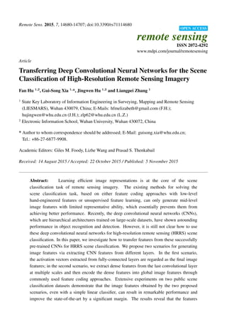
SlideShare a Scribd company logo
1 of 28
Download to read offline
Remote Sens. 2015, 7, 14680-14707; doi:10.3390/rs71114680
OPEN ACCESS
remote sensing
ISSN 2072-4292
www.mdpi.com/journal/remotesensing
Article
Transferring Deep Convolutional Neural Networks for the Scene
Classification of High-Resolution Remote Sensing Imagery
Fan Hu 1,2
, Gui-Song Xia 1,
*, Jingwen Hu 1,2
and Liangpei Zhang 1
1
State Key Laboratory of Information Engineering in Surveying, Mapping and Remote Sensing
(LIESMARS), Wuhan 430079, China; E-Mails: hfmelizabeth@gmail.com (F.H.);
hujingwen@whu.edu.cn (J.H.); zlp62@whu.edu.cn (L.Z.)
2
Electronic Information School, Wuhan University, Wuhan 430072, China
* Author to whom correspondence should be addressed; E-Mail: guisong.xia@whu.edu.cn;
Tel.: +86-27-6877-9908.
Academic Editors: Giles M. Foody, Lizhe Wang and Prasad S. Thenkabail
Received: 14 August 2015 / Accepted: 22 October 2015 / Published: 5 November 2015
Abstract: Learning efficient image representations is at the core of the scene
classification task of remote sensing imagery. The existing methods for solving the
scene classification task, based on either feature coding approaches with low-level
hand-engineered features or unsupervised feature learning, can only generate mid-level
image features with limited representative ability, which essentially prevents them from
achieving better performance. Recently, the deep convolutional neural networks (CNNs),
which are hierarchical architectures trained on large-scale datasets, have shown astounding
performance in object recognition and detection. However, it is still not clear how to use
these deep convolutional neural networks for high-resolution remote sensing (HRRS) scene
classification. In this paper, we investigate how to transfer features from these successfully
pre-trained CNNs for HRRS scene classification. We propose two scenarios for generating
image features via extracting CNN features from different layers. In the first scenario,
the activation vectors extracted from fully-connected layers are regarded as the final image
features; in the second scenario, we extract dense features from the last convolutional layer
at multiple scales and then encode the dense features into global image features through
commonly used feature coding approaches. Extensive experiments on two public scene
classification datasets demonstrate that the image features obtained by the two proposed
scenarios, even with a simple linear classifier, can result in remarkable performance and
improve the state-of-the-art by a significant margin. The results reveal that the features
Remote Sens. 2015, 7 14681
from pre-trained CNNs generalize well to HRRS datasets and are more expressive than
the low- and mid-level features. Moreover, we tentatively combine features extracted from
different CNN models for better performance.
Keywords: CNN; scene classification; feature representation; feature coding; convolutional
layer; fully-connected layer
1. Introduction
With1 the rapid increase of remote sensing imaging techniques over the past decade, a considerable
amount of high-resolution remote sensing (HRRS) images are now available, thereby enabling us to
study the ground surface in greater detail. Scene classification of HRRS imagery, which aims to
classify extracted subregions of HRRS images covering multiple land-cover types or ground objects
into different semantic categories, is a fundamental task and very important for many practical remote
sensing applications, such as land resource management, urban planing, and computer cartography,
among others [1–8]. Generally, some identical land-cover types or object classes are frequently shared
among different scene categories. For example, commercial area and residential area, which are two
typical scene categories, may both contain roads, trees and buildings at the same time but differ in the
density and spatial distribution of these three thematic classes. Hence, such complexity of spatial and
structural patterns in HRRS scenes makes scene classification a fairly challenging problem.
Constructing a holistic scene representation is an intuitively feasible approach for scene classification.
The bag-of-visual-words (BOW) model [9] is one of the most popular approaches for solving the scene
classification problem in the remote sensing community. It is originally developed for text analysis,
which models a document by its word frequency. The BOW model is further adapted to represent images
by the frequency of “visual words” that are constructed by quantizing local features with a clustering
method (e.g., K-means) [9,10]. Considering that the BOW representation disregards spatial information,
many variant methods [5,10–14] based on the BOW model have been developed for improving
the ability to depict the spatial relationships of local features. However, the performance of these
BOW-based methods strongly relies on the extraction of handcrafted local features, e.g., local structural
points [15,16], color histogram, and texture features [17–19]. Thus, some researchers introduced the
unsupervised feature learning (UFL) procedures [20], which can automatically learn suitable internal
features from a large amount of unlabeled data via specific unsupervised learning algorithms rather than
engineered features, for HRRS scene classification and achieved promising results.
Nevertheless, it appears that the performance of HRRS scene classification has only gained small
improvements in recent years, with proposing minor variants of successful baseline models, which
is mainly because the existing approaches are incapable of generating sufficiently powerful feature
representations for HRRS scenes. In fact, the BOW and UFL methods generate feature representations
in the mid-level form to some extent. Therefore, the more representative and higher-level features,
which are abstractions of the lower-level features and can exhibit substantially more discrimination,
are desirable and will certainly play a dominant role in scene classification task.
Remote Sens. 2015, 7 14682
Recently, the deep learning methods [21–23] have achieved great success not only in classic problems,
such as speech recognition, object recognition and detection, and natural language processing, but also
in many other practical applications. These methods have achieved dramatic improvements beyond the
state-of-the-art records in such broad domains, and they have attracted considerably interest in both
the academic and industrial communities [22]. In general, deep learning algorithms attempt to learn
hierarchical features, corresponding to different levels of abstraction. The deep convolutional neural
networks (CNNs) [24], which are acknowledged as the most successful and widely used deep learning
approach, are now the dominant methods in the majority of recognition and detection tasks due to the
remarkable results on a number of benchmarks [25–28]. CNN is a biologically inspired multi-stage
architecture composed of convolutional, pooling and fully-connected layers, and it can be efficiently
trained in a completely supervised manner. However, it is difficult to train a high-powered deep CNN
with small datasets in practice. At present, many recent works [29–34] have demonstrated that the
intermediate activations learned with deep CNNs pre-trained on large datasets such as ImageNet [35]
can be transferable to many other recognition tasks with limited training data. We can easily arrive
at the following question: can we transfer the successfully pre-trained CNNs to address HRRS scene
classification, which is also a typical recognition task with limited amount of training data? To our
knowledge, this question still remains unclear, except for the concurrent works [36,37] with ours.
In this paper, we investigate transferring off-the-shelf pre-trained CNNs for HRRS scene classification
and attempt to form better representations for image scenes from CNN activations. By removing the last
few layers of a CNN, we treat the remainder of the CNN as a fixed feature extractor. Considering that
these pre-trained CNNs are large multi-layer architectures, we propose two scenarios of extracting CNN
features with respect to different layers:
- we simply compute the CNN activations over the entire image scene and regard the activation
vectors of the fully-connected layer as the global feature representations for scenes;
- we first generate dense CNN activations from the last convolutional layer with multiple scales
of the original input image scenes, and then we aggregate the dense convolutional features into
a global representation via the conventional feature coding scheme, e.g., the BOW and Fisher
encoding. These dense CNN activations describe multi-scale spatial information.
After the feature extraction stage via the CNNs, the global features of the image scenes are fed into
a simple classifier for the scene classification task. Extensive experiments show that we can generate
powerful features for HRRS scenes through transferring the pre-trained CNN models and achieve
state-of-the-art performance on two public scene datasets with the proposed scenarios.
The main contributions of this paper are summarized as follows:
- We thoroughly investigate how to effectively use CNN activations from not only the
fully-connected layers but also the convolutional layers as the image scene features.
- We conduct a comparative evaluation of various pre-trained CNN models utilized for computing
generic image features
- A novel multi-scale feature extraction approach with the pre-trained CNN is presented, where
we encode the dense CNN activations from the convolutional layer to generate image scene
Remote Sens. 2015, 7 14683
representations via feature coding methods. Moreover, four commonly used feature coding
methods are evaluated based on the proposed approach.
- The two proposed scenarios achieve a significant performance enhancement compared to existing
methods on two public HRRS scene classification benchmarks and provide a referable baseline for
HRRS scene classification with deep learning methods.
The remainder of this paper is organized as follows. In Section 2, we briefly review some related
works corresponding to some state-of-the-art scene classification methods, CNN and transferring CNN
activations to visual recognition tasks. In Section 3, we introduce the classic architecture of CNNs and
some recently reported large CNNs used in our work. In Section 4, we present two scenarios of extracting
image representations using the pre-trained CNN model. Details of our experiments and the results are
presented in Section 5. Finally, we draw conclusions for this paper with some remarks. In addition,
we list the important items and their corresponding abbreviations in this paper, shown in Table 1, for a
quick and concise reference.
Table 1. List of Some Important Items and Corresponding Abbreviations.
HRRS High-Resolution Remote Sensing
CNN convolutional neural network
UFL unsupervised feature learning
SIFT scale invariant feature transformation
FC layer fully-connected layer
ReLU rectified linear units
ILSVRC ImageNet Large Scale Visual Recognition Challenge
AlexNet a CNN architecture developed by Alex Krizhevsky [25]
Caffe Convolutional Architecture for Fast Feature Embedding [28]
CaffeNet a CNN architecture provided by Caffe [28]
VGG-F a fast CNN architecture developed by Chatfield [33]
VGG-M a medium CNN architecture developed by Chatfield [33]
VGG-S a slow CNN architecture developed by Chatfield [33]
VGG-VD16 a very deep CNN architecture (16 layers) developed by Simonyan [27]
VGG-VD19 a very deep CNN architecture (19 layers) developed by Simonyan [27]
BOW bag of visual words
IFK improved Fisher kernel
LLC locality-constrained linear coding
VLAD vector of locally aggregated descriptors
SVM support vector machine
Remote Sens. 2015, 7 14684
2. Related Work
The bag-of-visual-words (BOW) model is a very popular approach in HRRS scene classification. In a
general pipeline of BOW, the local features of an image, such as SIFT features, are extracted first and then
each feature is encoded to its nearest visual word; the final image representation is a histogram where
each bin counts the occurrence frequency of local features on a visual word. Many researchers have
proposed improved variants of BOW based on the specific characteristics of HRRS scenes: Yang et al. [5]
proposed the spatial co-occurrence kernel (SCK) that describes the spatial distribution of visual words;
Chen et al. [13] proposed a translation and rotation-invariant pyramid-of-spatial-relations (PSR) model
to describe both relative and absolute spatial relationships of local features; Zhao et al. [11] proposed
a concentric circle-structured multi-scale BOW (CCM-BOW) model to achieve rotation-invariance;
and Cheng et al. [38] developed a rotation-invariant framework based on a collection of part detectors
(COPD) that can capture discriminative visual parts of images. Although these methods have achieved
good performance, they are essentially extensions of the classic BOW model, and it is difficult to achieve
considerable enhancements in performance due to the limited representative ability of these low- and
mid-level features.
Unsupervised feature learning (UFL) [20] has recently become a hot research topic in the machine
learning community. The UFL approaches automatically learn features from a large number of unlabeled
samples via unsupervised learning algorithms, which can discover more useful or discriminative
information hidden in the data itself. Several works that utilize UFL methods for HRRS scene
classification have been published. Cheriyadat [4] used the sparse coding algorithm to learn sparse local
features for image scenes and pool local features to generate image representations. Zhang et al. [39]
used a classic neural network, called sparse autoencoder, which is trained on a group of selective image
patches sampled by their saliency degree, to extract local features. Hu et al. [40] improved the classic
UFL pipeline by learning features on a low-dimensional image patch manifold. Although the UFL
methods are free of hand-engineered features, they still result in limited performance improvement
(and even worse than the BOW model) due to their shallow learning architectures.
Although we have recently witnessed the overwhelming popularity of CNNs, the original concept
of CNN dates back to Fukushima’s biologically inspired “neocognitron” [41], a hierarchical network
with invariance to image translations. LeCun et al. [24] were the first to successfully train the CNN
architecture based on the backpropagation algorithm, and they achieved leading results in character
recognition. CNNs were once largely forsaken by the academic community with the rise of support
vector machine (SVM). Dramatic breakthroughs on many challenging visual recognition benchmarks
have been achieved by the deep CNNs over the past few years, which has resulted in CNNs regaining
considerable popularity in the computer vision community [25,27,28,32,33,42]. However, it is very
difficult to train a deep CNN, which typically contains millions of parameters for some specific tasks,
with a small number of training samples. Increasingly more works have recently shown that intermediate
features extracted from deep CNNs that are trained on sufficiently large-scale datasets, such as ImageNet,
can be successfully applied to a wide range of visual recognition tasks, e.g., scene classification [29,43],
object detection [34,44] and image retrieval [25,43]. Almost all of the works utilize CNN activations
from the fully-connected layers, while the features from convolutional layer have not received sufficient
Remote Sens. 2015, 7 14685
attention. Cimpoi et al. [45] very recently showed impressive performance on texture recognition
by pooling CNN features from convolutional layers with Fisher coding, which demonstrates that the
activations from convolutional layers are also powerful generic features.
In the remote sensing field, there is still a lack of investigations on using CNNs for HRRS scene
classification; hence, we attempt to present a comprehensive study on this topic. Our work is most related
to [36,37], which are concurrent works with our own. In [37], the authors employed pre-trained CNNs
and fine-tuned them on the scene datasets, showing impressive classification performance, whereas we
transfer the pre-trained CNNs for scene datasets without any training modalities (fine-tuning or training
from scratch) and simply take the pre-trained CNNs as fixed feature extractors. In [36], the authors
evaluated the generalization power of CNN features from fully-connected layers in remote sensing image
classification and showed state-of-the-art results on a public HRRS scene dataset. In contrast to [36],
we investigate CNN features not only from fully-connected layers but also from convolutional layers,
we evaluate more pre-trained CNN models, and more detailed comparative experiments are presented
under various settings. Thus, this paper provides a more systematic study on utilizing pre-trained CNN
for HRRS scene classification tasks.
3. Deep Convolutional Neural Networks (CNNs)
The typical architecture of a CNN is composed of multiple cascaded stages. The convolutional
(conv) layers and pooling layers construct the first few stages, and a typical stage is shown in Figure 1.
The convolutional layers output feature maps, each element of which is obtained by computing a dot
product between the local region (receptive field) it is connected to in the input feature maps and a set
of weights (also called filters or kernels). In general, an elementwise non-linear activation function
is applied to these feature maps. The pooling layers perform a downsampling operation along the
spatial dimensions of feature maps via computing the maximum on a local region. The fully-connected
(FC) layers finally follow several stacked convolutional and pooling layers, and the last fully-connected
layer is a Softmax layer that computes the scores for each defined class. CNNs transform the input
image from original pixel values to the final class scores through the network in a feedforward manner.
The parameters of CNNs (i.e., the weights in convolutional and FC layers) are trained with classic
stochastic gradient descent based on the backpropagation algorithm [46].
In this section, we briefly review some successful modern CNN architectures evaluated in our work.
3.1. AlexNet
AlexNet, developed by Alex Krizhevsky et al. [25], is a groundbreaking deep CNN architecture and
a winning model in the 2012 ImageNet Large Scale Visual Recognition Challenge (ILSVRC-2012) [47].
In contrast to the early CNN models, AlexNet consists of five convolutional layers, the first, second and
fifth of which are followed with pooling layers, and three fully-connected layers, as shown in Figure 2.
The success of AlexNet is attributed to some practical “tricks”, such as Rectified Linear Units (ReLU)
non-linearity, data augmentation, and dropout. The ReLU, which is simply the half-wave rectifier
function f(x) = max(x, 0), can significantly accelerate the training phase; the data augmentation is
an effective way to reduce overfitting when training a large CNN, which generates more training image
Remote Sens. 2015, 7 14686
samples by cropping small-sized patches and horizontally flipping these patches from original images;
and the dropout technique, which reduces the co-adaptations of neurons by randomly setting zeros to
the output of each hidden neuron, is used in fully-connected layers to reduce substantial overfitting.
In summary, the success of AlexNet popularizes the application of large CNNs in visual recognition
tasks, and hence, AlexNet has become a baseline architecture of modern CNNs.
Convolution Non-Linearity Pooling
Figure 1. Illustration of a typical stage of a CNN. The convolutional layer is implemented
by convolving the input with a set of filters, followed by a elementwise non-linear function
(e.g., the ReLU non-linearity), and generates a group of feature maps, each of which
corresponds to the response of convolution between the input and a filter. The pooling layer,
if max-pooling used, outputs the maximal values of spatially successive local regions on the
feature maps. Its main function is to reduce the spatial size of feature maps and hence to
reduce computation for upper layers.
COV1
C1
C2
C3 C4 C5
FC6 FC7
55
96
5
5
27
256
384 384 256
4096
FC8
4096
1000
13 13 13
3
3
3
3
5
5
C1
C2
C3 C4 C5
FC6 FC7
55
96
5
5
27
256
384 384 256
4096
FC8
4096
1000
13 13 13
3
3
3
3
3
3
55
27
13 13 13
Figure 2. The overall architecture of AlexNet. It is composed of five convolutional
layers (C1−C5) and three FC layers (FC6−FC8), which becomes the baseline model of
modern CNNs.
Remote Sens. 2015, 7 14687
3.2. CaffeNet
The Convolutional Architecture for Fast Feature Embedding, also called Caffe [28], is a
open-source deep learning framework that provides clean, modifiable and possibly the fastest available
implementations for effectively training and deploying general-purpose CNNs and other deep models.
In this paper, we will use the pre-trained CNN provided by Caffe (CaffeNet for short), which has a
very similar architecture with AlexNet except for two small modifications: (1) training without data
augmentation and (2) exchanging the order of pooling and normalization layers. CaffeNet was also
trained on the ILSVRC-2012 training set and achieved performance close to that of AlexNet.
3.3. VGGNet
To evaluate the performance of different deep CNN models and compare them on a common ground,
Chatfield et al. [33] developed three CNN architectures based on the Caffe toolkit, each of which
explores a different speed/accuracy trade-off:
(1) VGG-F: The fast CNN architecture is similar to AlexNet. The primary differences from AlexNet
are the smaller number of filters and small stride in some convolutional layers.
(2) VGG-M: The medium CNN architecture is similar to the one presented by Zeiler et al. [32]. It is
constructed with a smaller stride and pooling size in the 1st convolutional layer. A smaller number
of filters in the 4th convolutional layer is explored for balancing the computational speed.
(3) VGG-S: The slow CNN architecture is a simplified version of the accurate model in the OverFeat
framework [26], which retains the first five convolutional layers of the six layers in the original
accurate OverFeat model and has a smaller number of filters in the 5th layer. Compared to the
VGG-M, the main differences are the the small stride in the 2nd convolutional layer and the large
pooling size in the 1st and 5th convolutional layers.
3.4. VGG-VD Networks
Simonyan et al. [27] developed the very deep CNN models that won the runner-up in ILSVRC-2014.
The impressive results of the two very deep CNNs, known as VGG-VD16 (containing 13 convolutional
layers and 3 fully-connected layers) and VGG-VD19 (containing 16 convolutional layers and
3 fully-connected layers ), demonstrate that the depth of the network plays a significant role in improving
classification accuracy. The VGG-VD networks are also very popular candidate models for extracting
CNN activations of images.
3.5. PlacesNet
PlacesNet, which was developed by Zhou et al. [48], has an identical architecture with CaffeNet.
It was trained on the Places database, a large-scale scene-centric dataset with 205 natural scene
categories, rather than on ImageNet. The authors showed that the deep features from PlacesNet are more
effective for recognizing natural scenes than deep features from CNNs trained on ImageNet. We will
evaluate PlacesNet to verify whether it results in excellent performance on the HRRS scene benchmark.
Remote Sens. 2015, 7 14688
4. Methodology of Transferring Deep CNN Features for Scene Classification
As mentioned previously, the activations from high-level layers of pre-trained CNNs have proven to be
powerful generic feature representations with excellent performance. However, in almost all published
works, only the 4096-dimensional activations of the penultimate layer are widely used as the final image
features. Features extracted from lower-level layers, particularly the convolutional layers, lack sufficient
study. In this section, we propose two scenarios for utilizing deep CNN features for scene classification
for the sake of investigating the effectiveness of deep features from convolutional layers and FC layers,
which are illustrated in Figure 3.
C1
C2
C3 C4 C5
FC6 FC7
C1 C2 C3 C4 C5
Pre-trained CNN
Output C5 Activations
C1 C2 C3 C4 C5
C1 C2 C3 C4 C5
Multiple Scales Dense Features
GlobalRepresentation
Pre-trained CNN
Output FC6/FC7 Activations
Feature Coding
GlobalRepresentation
(I)
(II)
Figure 3. Illustration of the two proposed scenarios for generating global feature
representations for scene classification. Both of the scenarios utilize the deep CNN features,
but from different layers. In scenario (I), we extract the activations from the first or second
FC layer and consider the 4096-dimensional feature vector as the final image representation;
In scenario (II), we construct the global image representation by aggregating multi-scale
dense features via feature coding approaches.
4.1. Scenario (I): Utilize Features from FC Layers
Following the standard pipeline of previous works, we remove the last FC layer (the Softmax layer)
of a pre-trained CNN and treat the rest of the CNN as a fixed feature extractor. By feeding an input
image scene into the CNN, we directly compute a 4096-dimensional activation vector from the first
or second FC layer in a feedforward way and consider the vector as a global feature representation of
the input image. Finally, we implement scene classification by training a linear SVM classifier with
the 4096-dimensional features. Although this scenario is very straightforward, several practical details
should be taken into consideration:
- Because all the pre-trained CNNs require a fixed-size (e.g., 224 × 224) input image, we should
beforehand resize each image scene to the fixed size by feeding it into the network. The size
Remote Sens. 2015, 7 14689
constraint causes inevitable degradation in spatial resolution when the original size of the image is
larger than the pre-defined size of the CNN.
- Although data augmentation is an effective technique to reduce overfitting in the training stage,
recent works show that in the testing stage, data augmentation, which is performed by sampling
multiple sub-image windows and averaging the activations of these sub-images, also helps to
improve classification performance. In this paper, we also apply the prevalent “center + corners
with horizontal flips” augmentation strategy [25,32,33] to increase accuracy. We extract five
sub-image windows (with the required size of the CNN), corresponding to the center and four
corners, as well as their horizontal flips, and then we construct the global feature for each image
by averaging the activation vectors over the ten sub-image windows.
- As a common practice, the 4096-dimensional output features should go through the ReLU
transformation so that all the elements of the features are non-negative. We have also evaluated
the features without ReLU but achieved slightly worse performance.
4.2. Scenario (II): Utilize Features from Convolutional Layers
In contrast to the popularity of the CNN features from FC layers, the features from intermediate
convolutional layers appear to lack practical use. Although the features of FC layers capture global
spatial layout information, they are still fairly sensitive to global rotation and scaling, making them less
suitable for HRRS scenes that greatly differ in orientation and scales. Therefore, we regard the feature
maps produced by convolutional layers as dense features and aggregate them via the orderless feature
coding approach [49,50].
In scenario (II), by removing all FC layers, we output the feature maps from the last convolutional
layer. Each entity along the feature maps can be considered as a “local” feature, and the length of
the feature equals the number of feature maps. As discussed in [44], the requirement of fixed-size
images comes only from FC layers, and convolutional layers do not require images to have a fixed
size. Due to not involving FC layers in scenario (II), we can freely extract convolutional features for
an input image with any size. Here, we propose to extract multi-scale dense convolutional features by
feeding input images of multiple sizes into the pre-trained CNN to capture multi-scale information in
the HRRS scene. Let the F
(m)
s be the set of dense convolutional features extracted from image Im at
scale index s. We then obtain a complete feature set by combining all F
(m)
s at different scales, which
is denoted as F(m)
= [x1, x2, · · · , xN ] ∈ RD×N
consisting of N D-dimensional features. Here, we
introduce four conventional feature coding methods, which are BOW [9], locality-constrained linear
coding (LLC) [51], improved Fisher kernel (IFK) [52] and vector of locally aggregated descriptors
(VLAD) [53], to encode the feature set F(m)
into a global feature representation for each image Im.
Note that the BOW, LLC and VLAD encode features based on a codebook constructed via K-means,
whereas the IFK encodes features with a probability density distribution described by the Gaussian
mixture model (GMM). After generating the global feature for each image scene, we directly implement
the scene classification with a simple linear SVM for training and testing.
Remote Sens. 2015, 7 14690
5. Experiments and Analysis
In this section, we investigate the representative power of CNN features and evaluate the two proposed
scenarios of transferring CNN features for HRRS scene classification with various pre-trained CNN
models. The detailed experimental setup and numerous experiments with reasonable analysis are
also presented.
5.1. Experimental Setup
We evaluate the effectiveness of deep CNN features on the following two publicly available land
use datasets:
- UC Merced Land Use Dataset. The UC Merced dataset (UCM) [5], manually collected from large
aerial orthoimagery, contains 21 distinctive scene categories. Each class consists of 100 images
with a size of 256 × 256 pixels. Each image has a pixel resolution of one foot. Figure 4 shows
two examples of each category included in this dataset. Note that this dataset shows very small
inter-class diversity among some categories that share a few similar objects or textural patterns
(e.g., dense residential and medium residential), which makes the UCM dataset a challenging one.
- WHU-RS Dataset. The WHU-RS dataset [6], collected from Google Earth (Google Inc.), is a new
publicly available dataset, which consists of 950 images with a size of 600 × 600 pixels uniformly
distributed in 19 scene classes. Some example images are shown in Figure 5. We can see that the
variation of illumination, scale, resolution and viewpoint-dependent appearance in some categories
makes it more complicated than the UCM dataset.
Agricultural Airplane Baseball Diamond Beach Buildings Chaparral Dense Residential
Forest Freeway Golf Course Harbor Intersection Medium Residential Mobile Home Park
Overpass Parking Lot River Runway Sparse Residential Storage Tanks Tennis Courts
Figure 4. Two examples of each scene category in the UC Merced dataset.
For experiments in scenario (I), all the pre-trained CNN models introduced in Section 3 are evaluated
and compared. Considering the pre-defined size requirements of the input image of these CNNs,
we resize all images to 227 × 227 for AlexNet, CaffeNet, and PlacesNet and to 224 × 224 for the other
CNNs. The only preprocessing we conduct is subtracting the per-pixel mean value (with RGB channels)
computed on the training set from each pixel, which is a conventional stage prior to computing CNN
activations [25,27,32,43]. The final 4096-dimensional feature vectors from the first or second FC layer
are fed into a linear SVM classifier without any normalization. In the data augmentation case, we crop
10 sub-images (center, four corners, and their horizontal flips) according to the required size, and we
Remote Sens. 2015, 7 14691
also pre-process the crops by mean subtraction. For each image scene, we average the 4096-dimensional
activations made by its 10 sub-images to generate a resulting image representation.
Airport Beach Bridge Commercial Desert
Farmland Football Field Forest Industrial Meadow
Mountain Park Parking Lot Pond Port
Railway Residential River Viaduct
Figure 5. Examples of each category in the WHU-RS dataset.
For experiments in scenario (II), we evaluate the dense CNN features of CaffeNet, VGG-M and
VGG-VD16 with the four feature coding methods mentioned above. The dense CNN features without
ReLU are extracted from the last convolutional layer by default. We set three different image scales to
generate multi-scale dense features: 128×128, the original 256×256 and 512×512 for the UCM images
and 150 × 150, 300 × 300, and the original 600 × 600 for the WHU-RS images. In fact, too small or too
large scale factors do not result in better performance. Input images with a scale that is too small lead
to very small feature maps from the last convolutional layer (after several stages of convolution-pooling,
the spatial resolution of feature maps is greatly reduced), which makes the following feature coding
stage ineffective; images with a scale that is too large result in many redundant features in the feature
maps, which has a negative effect on the final performance. Moreover, images with a scale that is too
large make the process of extracting CNN features very slow. In general, image scales ranging from
100 × 100 to 1000 × 1000 are appropriate settings by experience. The dense features are L2-normalized
prior to applying feature coding. Although the encoding stages of BOW, LLC and VLAD all rely on the
codebook learned by K-means clustering, we set different numbers of codewords empirically, which are
Remote Sens. 2015, 7 14692
assigned to be 1000, 10,000, and 100 with respect to each method, for the purpose of achieving good
performance. The number of Gaussian components in the GMM with which the IFK encodes features is
empirically set to be 100.
We randomly select samples of each class for training the SVM classifier and the rest for testing,
following the same sampling setting as [5,54] for the two datasets, respectively: 80 training samples per
class for the UCM dataset and 30 training samples per class for the WHU-RS dataset. The classification
accuracy is measured by A = Nc/Nt, where Nc denotes the number of correctly classified samples in the
testing samples and Nt denotes the total number of testing samples. We evaluate the final classification
performance with the average accuracy A over 50 runs (each run with randomly selected training and
testing samples). The public LIBLINEAR library [55] is used for SVM training and testing with the
linear kernel. We also use the open source library VLFeat [56] for implementing the feature coding
methods and Caffe for extracting CNN features. The pre-trained CNN models used in this paper are
available in the Caffe Model Zoo [57] with a 2.4 GHz quad-core Intel Core i7 CPU and a GeForce GT
750M 2 GB GPU.
5.2. Experimental Results of Scenario (I)
We first test CNN features from the second FC layers, which is a general case used in many works.
The classification performances of scenario (I) with eight different pre-trained CNN models are shown
in Table 2. The resulting high classification accuracies reveal the powerful ability of pre-trained
CNNs transferred from the ImageNet dataset to HRRS scene datasets. The VGG-S features achieve
the best results on both UCM and WHU-RS and slightly outperform the features of VGG-M and
VGG-F, which have architectures similar to that of the VGG-S. The VGG-VD networks, which consist
of considerably more layers and achieve better performance on many natural image classification
benchmarks than other shallow CNN models, do not achieve results as good as expected and even
perform worse than the baseline AlexNet on HRRS. PlacesNet, which consistently outperforms AlexNet
on natural scene datasets, performs considerably worse than AlexNet, revealing that the structural and
textural patterns in HRRS scenes are very different from those in natural scenes.
We also present the classification results of CNN features from the first FC layer, shown in Table 3.
It is obvious that features extracted from the first FC layer result in slightly better performance than
features from the second layer with different CNNs, which is probably caused by the fact that the earlier
layers of a CNN contain more generic features that are useful for other datasets. The effect of data
augmentation is verified in Table 3. The better performance achieved with data augmentation in all cases
confirms that it is a simple but effective technique for increasing performance. We also note that the
VGG-S model consistently outperforms other CNNs, except for the case about features from the first FC
layer with data augmentation on UCM where the VGG-VD16 achieves the best accuracy.
Remote Sens. 2015, 7 14693
Table 2. Performance Comparison of CNN Features (from the second layer) of Various
Pre-trained CNN Models.
Pre-Trained CNN
Classification Accuracy (%)
UCM WHU-RS
AlexNet 94.37 93.81
CaffeNet 94.43 94.54
VGG-F 94.35 95.11
VGG-M 94.48 94.98
VGG-S 94.60 95.46
VGG-VD16 94.07 94.35
VGG-VD19 93.15 94.36
PlacesNet 91.44 91.73
Table 3. Performance Comparison of CNN Features (from the first FC layer) and the Effect
of Data Augmentation.
Pre-Trained CNN
UCM WHU-RS
1st-FC 1st-FC+Aug 2nd-FC+Aug 1st-FC 1st-FC+Aug 2nd-FC+Aug
AlexNet 95.08 95.57 95.20 94.29 95.69 95.49
CaffeNet 95.09 95.88 95.17 95.52 96.23 95.58
VGG-F 95.19 96.24 95.54 95.69 95.94 95.50
VGG-M 95.64 96.47 95.68 95.89 96.34 95.43
VGG-S 95.66 96.69 96.01 96.28 96.71 95.85
VGG-VD16 95.43 96.88 95.42 95.21 95.75 95.22
VGG-VD19 94.60 96.58 95.40 95.36 96.16 95.37
PlacesNet 93.33 94.90 92.61 92.68 94.89 93.23
We evaluate the time consumption (measured in terms of seconds) of computing CNN features with
each pre-trained CNN model for all image scenes in the UCM dataset, shown in Figure 6. As expected,
AlexNet, CaffeNet, VGG-F and PlacesNet have almost the same computational cost due to their very
similar architectures (actually, CaffeNet and PlacesNet share an identical architecture). Because the
layers of VGG-VD16 and VGG-VD19 are considerably more than the other CNNs, the two models lead
to far more time consumption.
To intuitively understand the CNN activations, we visualize the representations of each layer by
inverting them into reconstruction images with the technique proposed in [58], shown in Figure 7a.
It is very interesting that (1) the features of convolutional layers can be reconstructed to images similar
to the original image, with more blurs as progressing to deeper layers; and (2) although the features of
FC layers cannot be inverted to a recognizable image, the reconstructed images contain many similar
meaningful parts (e.g., the wings of airplanes) that are randomly distributed. These results show that
FC layers rearrange the information from low-level layers to generate more abstract representations.
More reconstruction examples are shown in Figure 7b. In addition, we report the reconstruction results
Remote Sens. 2015, 7 14694
of a local region on feature maps from different convolutional layers, which are shown in Figure 8.
We can see that the size of the receptive filled with respect to the input image becomes larger for the
neurons on feature maps of deeper layers.
0
100
200
300
400
500
RunningTime(s)
AlexNet
CaffeNet
VGG−F
VGG−M
VGG−S
VGG−VD16
VGG−VD19
PlacesNet
Figure 6. The time consumption of computing CNN activations with different CNN models
for all image scenes in the UCM dataset. In this evaluation, the CNN activations from the
first FC layer are extracted.
conv1 relu1 pool1 norm1 conv2 conv3norm2pool2relu2 relu3
conv4 relu4 conv5 relu5 pool5 relu7fc7relu6fc6 fc8
Parking Lot
Airport
conv1 relu1 pool1 norm1 conv2 conv3norm2pool2relu2 relu3
conv4 relu4 conv5 relu5 pool5 relu7fc7relu6fc6 fc8
pool2
pool5
pool2
pool5
Originalconv5pool5
(1) (2) (3) (4) (5) (6) (7) (8)
(a)
pool1 norm1 conv2 conv3norm2pool2relu2 relu3
conv5 relu5 pool5 relu7fc7relu6fc6 fc8
pool1 norm1 conv2 conv3norm2pool2relu2 relu3
conv5 relu5 pool5 relu7fc7relu6fc6 fc8
Originalconv5pool5
(1) (2) (3) (4) (5) (6) (7) (8) (9)
(b)
Figure 7. Reconstruction of CNN activations from different layers of AlexNet. The method
presented in [58] is used for visualization. The reconstructed images lose more details
increasingly along with deeper layers. (a) Reconstructed images from each layer of the
AlexNet; Reconstructed images from each layer of the AlexNet; (b) More reconstruction
examples of inverting CNN activations from the fifth convolutional and pooling layer.
Remote Sens. 2015, 7 14695
relu3 conv4 relu4 pool5relu5conv5
conv1 relu1 pool1 norm1 conv2 pool2relu2
norm2 conv3 relu3 conv4 relu4 pool5relu5conv5
Original
Figure 8. Reconstructed images from a local 5×5 region of feature maps at different layers.
We use the method proposed in [58] to visualize reconstructed images. At deeper layers,
the local region corresponds to a larger receptive field on the input image and thus results in
more complete reconstruction.
5.3. Experimental Results of Scenario (II)
5.3.1. Comparison of Feature Coding Methods
The overall performance of the BOW, VLAD, IFK and LLC when using different pre-trained CNNs
to extract dense convolutional features are shown in Table 4. Notably, the simplest BOW method leads
to such a high accuracy with dense CNN features and is generally comparable to the complex VLAD and
IFK. The best accuracy of BOW on UCM (96.51%, with VGG-VD16) exceeds all the results of using FC
features without data augmentation, and it is very close to the best one (96.88%, with data augmentation);
the best accuracy of BOW on WHU-RS (98.10%, with VGG-VD16) exceeds all results even with data
augmentation. The IFK works slightly better than the BOW and VLAD on the two datasets, except
the best result (98.64%) produced by VLAD with VGG-VD16, whereas the LLC performs worst in all
cases. We also obtain interesting results for VGG-VD16, which performs worse than the other CNN
models when using FC features (in Table 2) and works very well (better than CaffeNet, comparable to
VGG-M) when using convolutional features. A possible explanation is that the FC features of VGG-VD
models are more specific to categories in the ImageNet dataset, whereas the convolutional features are
more generalized to other datasets.
Table 4. Overall Classification Accuracy of Four Feature Coding Methods Using Different
Pre-trained CNNs.
Feature Coding
Method
UCM WHU-RS
CaffeNet VGG-M VGG-VD16 CaffeNet VGG-M VGG-VD16
BOW 95.16 96.11 96.51 96.36 98.02 98.10
VLAD 95.39 96.04 96.46 96.55 97.88 98.64
IFK 95.71 96.90 96.52 97.43 98.28 97.79
LLC 94.50 95.24 95.64 96.06 96.97 97.57
Remote Sens. 2015, 7 14696
For further comparison of the two proposed scenarios, we report the classification performance with a
varying number of training samples, as shown in Figure 9. We observe that the two scenarios consistently
achieve highly comparable accuracies on UCM, whereas scenario (II) outperforms scenario (I) by an
obvious margin on WHU-RS. This result is possibly caused by the following reason: in experiments in
scenario (I), because the sizes of the images (256 × 256) in UCM are very close to the required size
(224 × 224 or 227 × 227) of these CNNs, the resizing operation leads to little information loss; however,
for images in WHU-RS, we inevitably lose a considerable amount of information through rescaling
images of 600×600 pixels to the required size. Hence, the performance of scenario (I) on UCM is not as
good as that on WHU-RS. Overall, the proposed scenario (II) works better than scenario (I), particularly
for the dataset composed of large-sized images.
10 20 30 40 50 60 70 80
82
84
86
88
90
92
94
96
98
Number of training samples
AverageAccuracy(%)
Scenario I (VGG−S)
Scenario I (CaffeNet)
Scenario II (BOW)
Scenario II (VLAD)
5 10 15 20 25 30
88
90
92
94
96
98
100
Number of training samples
AverageAccuracy(%)
Scenario I (VGG−S)
Scenario I (CaffeNet)
Scenario II (BOW)
Scenario II (VLAD)
(a) (b)
Figure 9. Performance on two datasets with a varying number of training samples. Here,
we use the VGG-VD16 model to extract dense features for the BOW and VLAD of scenarios
(II). (a) Performance on the UCM dataset; (b) Performance on the WHU-RS dataset.
5.3.2. Effect of Image Scales
The results reported in Table 4 were obtained using convolutional features with respect to three image
scales. Here, to verify the effectiveness of this empirical setting, we also evaluate the performance
using IFK under several different scale settings, which are shown in Table 5. We can see that the three
scales generally lead to the highest accuracies, except being slightly worse than two scales when using
CaffeNet. One scale (i.e., the original image) and four scales do not work as well as three scales.
Hence, we conclude that in contrast to single-scale dense convolutional features, multi-scale features are
beneficial for increasing the classification accuracies, but the dense features of excessive scales may have
a negative effect on accuracies due to the considerable redundancy of features.
Remote Sens. 2015, 7 14697
Table 5. Classification Accuracy on the UCM Dataset of Dense CNN Features under
Different Scale Settings.
Scale Setting CaffeNet VGG-M VGG-VD16
One scale
(256×256)
95.08 96.28 93.97
Two scales
(128×128,256×256)
96.13 96.59 95.00
Four scales
(128×128,256×256, 512×512,1024×1024)
95.07 95.64 96.38
5.3.3. Effect of Different Convolutional Layers
Although we have achieved remarkable performance with dense features from the last convolutional
layer, from which convolutional layer the dense feature extracted can lead to the best accuracy is
worth discussing. The results of dense features extracted from each convolutional layer of the VGG-M
architecture are shown in Figure 10. It is clear that the classification accuracy increases progressively
along with the depth of the layers. As expected, features from the fifth convolutional layer (i.e., the last
one) result in the best accuracies on both of the datasets. This experiment also demonstrates the fact that
features of high-level layers are an abstraction of those of low-level layers and are more discriminative
for the classification task. Moreover, we observe that the IFK consistently outperforms the other three
methods; in particular, when features are extracted from the first convolutional layers, IFK features are
superior to the others by a large margin, which indicates that the IFK is a suitable approach for encoding
less representative features.
conv1 conv2 conv3 conv4 conv5
75
80
85
90
95
100
AverageAccuracy(%)
BOW
VLAD
IFK
LLC
conv1 conv2 conv3 conv4 conv5
75
80
85
90
95
100
AverageAccuracy(%)
BOW
VLAD
IFK
LLC
(a) (b)
Figure 10. Classification performance on two datasets of dense CNN features extracted from
each convolutional layer using different feature coding methods. Here, the VGG-M model is
evaluated. The lengths of CNN features from the first to the last convolutional layer are 96,
256, 512, 512, and 512. (a) Performance on the UCM dataset for each convolutional layer;
(b) Performance on the WHU-RS dataset for each convolutional layer.
Remote Sens. 2015, 7 14698
5.3.4. Comparison with Low-Level Features
To demonstrate the discriminative ability of dense CNN features, we compare them with the most
classic low-level features - SIFT descriptors. We proceed through the same pipeline of scenario (II)
using dense SIFT features (extracted from overlapping local image patches) rather than dense CNN
features, and the performances of SIFT features are shown in Table 6. For each feature coding method,
the best results of dense CNN features from CaffeNet, VGG-M and VGG-VD16 (as reported in Table 4)
are compared with the SIFT features. We can see that the dense CNN features outperform SIFT by a
significant ∼12% accuracy margin in the IFK case and by a ∼20% margin in the other three cases, which
reveals the substantial superiority in the representative ability of dense CNN features. Figure 11 shows
the confusion matrices of IFK with SIFT features and dense CNN features. The dense CNN features
result in 100% accuracy for most of the scene categories and largely improve performance in such
categories: airplane (55%→100%), dense residential (70%→90%), and storage tanks (35%→80%).
Table 6. Performance Comparison between SIFT Features and Dense CNN Features on the
UCM dataset.
SIFT Features Dense CNN Features
BOW 75.11 96.51
VLAD 74.50 96.46
IFK 84.40 96.90
LLC 77.64 95.64
0.95
0.05
0.05
0.80
0.15
0.05
0.05
0.10
0.10
0.55
0.05
0.25
0.05
0.05
1.00
0.65
0.10
0.15
1.00
0.05
0.70
0.15
0.05
0.95
0.05
0.05
0.80
0.10
0.05
0.10
0.85
0.05
0.05
1.00
0.05
0.95
0.20
0.05
0.05
0.70
0.05
0.10
0.90
0.05
0.10
0.05
0.90
0.05
1.00
0.05
0.85
0.05
0.05
0.05
0.05
1.00
0.05
0.05
0.05
0.10
0.05
0.75
0.10
0.05
0.20
0.35
0.05
0.05
0.70
AG
R
I
AIR
BASE
BEAC
HBU
ILD
C
H
AP
D
R
ES
FO
R
FR
EE
G
O
LF
H
AR
B
IN
TER
M
R
ES
M
PH
O
VER
PAR
K
R
IV
R
U
N
S
R
ES
STO
R
TEN
N
AGRI
AIR
BASE
BEACH
BUILD
CHAP
D RES
FOR
FREE
GOLF
HARB
INTER
M RES
MPH
OVER
PARK
RIV
RUN
S RES
STOR
TENN
(a)
Figure 11. Cont.
Remote Sens. 2015, 7 14699
1.00
0.05
0.95
0.05
1.00
1.00
1.00
0.05
0.05
1.00
0.90
0.05
1.00
0.05
0.95
1.00
1.00
0.05
0.90
0.05
0.10
0.85
1.00
1.00
1.00
0.05
1.00
0.10
0.05
1.00
0.05
0.10
0.85
0.80
0.95
AG
R
I
AIR
BASE
BEAC
HBU
ILD
C
H
AP
D
R
ES
FO
R
FR
EE
G
O
LF
H
AR
B
IN
TER
M
R
ES
M
PH
O
VER
PAR
K
R
IV
R
U
N
S
R
ES
STO
R
TEN
N
AGRI
AIR
BASE
BEACH
BUILD
CHAP
D RES
FOR
FREE
GOLF
HARB
INTER
M RES
MPH
OVER
PARK
RIV
RUN
S RES
STOR
TENN
(b)
Figure 11. Confusion matrices on the UCM dataset using IFK with SIFT features and dense
CNN features. (a) Confusion matrix of IFK with SIFT features; (b) Confusion matrix of IFK
with dense CNN features.
(a) (b) (c)
Figure 12. 2-D feature visualization of image global representations of the UCM dataset.
The t-SNE proposed in [59] is used to visualize the high-dimensional image representations.
The image representations are generated from (a) IFK with SIFT features; (b) features of the
first FC layer; and (c) IFK with dense features from the last convolutional layer. The VGG-M
model is used for (b) and (c). Each point on the graphs represents the 2-D feature of an image
in the dataset. Each color represents a different category in the dataset. (a) IFK with SIFT
features; (b) FC features of VGG-M; (c) IFK with dense CNN features of VGG-M.
In addition, we visualize the image global representations encoded via IFK with SIFT features
and dense CNN features for the UCM dataset. The image representations from the first FC layer
(i.e., scenarios (I)) are also visualized for comparison. Here, we first compute features for all image
Remote Sens. 2015, 7 14700
scenes in the dataset, and then we use the t-SNE algorithm [59] to embed the high-dimensional image
features on a 2-D space. We show these 2-D embedding points with different colors corresponding to
their actual scene categories. The final visualization results are shown in Figure 12. Notably, without
any training phases, the 2-D features from scenarios (I) and (II) naturally tend to form clusters that are
clearly separated. In contrast, the 2-D features via IFK with SIFT features only form a few visible
clusters, and many of the features overlap with each other in a confused order. This observation is
compatible with the common knowledge of deep learning that CNN features extracted from both FC
layers and convolutional layers are high-level features that contain more abstract semantic information,
whereas the hand-crafted features are only low-level features.
Table 7. Performance Comparison of State-of-the-art Methods on the UCM Dataset.
Methods Accuracy (%)
SPM [10] 74
SCK [5] 72.52
SPCK++ [12] 77.38
SC+Pooling [4] 81.67 ± 1.23
SG+UFL [39] 82.72 ± 1.18
CCM-BOVW [11] 86.64 ± 0.81
PSR [13] 89.1
UFL-SC [40] 90.26 ± 1.51
MSIFT [60] 90.97 ± 1.81
COPD [38] 91.33 ± 1.11
Dirichlet [61] 92.8 ± 0.9
VLAT [14] 94.3
CaffeNet [36] 93.42 ± 1.00
OverFeat [36] 90.91 ± 1.19
GoogLeNet+Fine-tune [37] 97.10
Scenario (I) 96.88 ± 0.72
Scenario (II) 96.90 ± 0.77
5.4. Comparison with State-of-the-Art Methods
As shown in Table 7, we compare our best results achieved via scenarios (I) and (II) with various
state-of-the-art methods that have reported classification accuracy on the UCM dataset. As expected,
the two proposed scenarios largely outperform all the methods except for the GoogLeNet+Fine-tune
approach [37]. In contrast with most of these methods that use a sophisticated learning strategy with
low-level hand-engineered features and non-linear classifiers, our methods are more straightforward and
simple: (1) conveniently extracting features from FC layers or convolutional layers of a pre-trained CNN
and (2) using the simple linear classifier to train and test. Moreover, as shown in Figure 9a, even with a
very small number of training samples, our methods still achieve greater than 91% accuracies (91.62%
with VGG-S of scenario (I) and 91.82% with BOW of scenario (II)), which exceed the majority of
existing methods. Although the proposed methods perform slightly worse than the method presented
in [37], directly comparing our methods with it is not fair. The GoogLeNet+Fine-tune approach fine
tunes the pre-trained CNN (GoogLeNet [42]) on the target dataset, whereas we only extract CNN
Remote Sens. 2015, 7 14701
activations in a straightforward way by feeding an image without changing the parameters of the
pre-trained CNN. On the WHU-RS dataset, our methods achieved considerably better performance
(96.71% of scenario (I) and 98.64% of scenario (II)) than the method (93.6%) presented in [54]. Overall,
remarkable classification results on the public benchmark are obtained by the two proposed scenarios
with CNN features, which are superior to almost all reported results with a substantial gain.
5.5. Combining Features from Two Scenarios
In previous experiments, we generated the global image representations via scenario (I) or (II)
solely. We can absolutely move a step further to combine the features computed by these two
frameworks. Due to the large difference in the scales and length, we should pre-process these two types
of global features before concatenating them. For scenario (I), the 4096-dimensional image features are
L2-normalized; for scenario (II), we perform PCA on the image features (which generally have quite
high dimensionality of more than 50K) and reduce them to 4096 dimensions, followed by normalizing
them with L2 normalization. Note that we do not apply PCA to image features encoded by the BOW
because the resulting features are only 1000-dimensional according to our default experimental setting.
After normalization and dimension reduction, we finally concatenate the two features to form a new
image representation. Here, we present some tentative combinations using different pre-trained CNNs
or feature coding approaches, and the results are shown in Table 8. We observe that on the UCM
dataset, the combined features improve performance with approximately 1%–2% gains compared to
the separate cases, whereas they only achieve marginal improvement on the WHU-RS dataset. Although
in [36], the authors achieve better performance by directly concatenating feature vectors from FC layers
computed by two pre-trained CNNs (CaffeNet and OverFeat), we believe that better performance can be
obtained through more complementary combinations.
Table 8. Performance of Combining Features Generated by the Two Scenarios (I) and (II).
Some Tentative Combinations are Provided.
Combination Classification Accuracy (%)
Scenario (I) Scenario (II) UCM WHU-RS
VGG-S BOW(VGG-M) 97.30 98.72
VGG-S VLAD(VGG-M) 97.92 98.79
VGG-S IFK(VGG-M) 98.27 98.70
VGG-S BOW(VGG-VD16) 98.05 98.82
VGG-S VLAD(VGG-VD16) 97.99 98.63
VGG-S IFK(VGG-VD16) 98.49 98.52
CaffeNet BOW(CaffeNet) 96.90 98.15
CaffeNet VLAD(CaffeNet) 97.31 98.21
CaffeNet IFK(CaffeNet) 97.40 98.03
CaffeNet BOW(VGG-VD16) 98.07 98.89
CaffeNet VLAD(VGG-VD16) 97.91 98.65
CaffeNet IFK(VGG-VD16) 98.16 98.80
OverFeat + CaffeNet [36] 99.43 –
Remote Sens. 2015, 7 14702
6. Discussion
From the extensive experiments above, the two proposed scenarios, which utilize CNN activations
from the FC layers and convolutional layers, respectively, have been proven to be very effective
for HRRS scene classification. Specifically, several interesting yet practical observations from the
experiments are summarized as follows:
- The features extracted from both FC layers and convolutional layers have stronger representative
ability than low-level hand-crafted features. Combined with a simple linear classifier, these CNN
features can result in very remarkable performance, which also reveals that the deep CNNs trained
on large natural image datasets generalize well to HRRS datasets.
- As shown in Figure 7, we can invert the CNN features from very deep layers (e.g., the fifth
convolutional layer) to recognizable reconstructed images. This result indicates that even from
a very deep layer, the extracted CNN features still preserve rich useful information, sufficient for
describing images.
- For HRRS scene datasets, due to their more generic ability, CNN features from the first FC layers
consistently work better than those from the second FC layers that are widely used in many works.
Moreover, the data augmentation technique is verified to be beneficial for increasing the final
classification performance.
- The selection of the pre-trained CNN model also influences the final performance. Overall,
the VGG-S model results in the best performance among the eight evaluated CNN models when
extracting FC features; the VGG-M model that balances accuracy and computational cost is a better
choice when extracting dense convolutional features. Moreover, PlacesNet, which is specially
trained with a large natural scene dataset and has achieved impressive results on many natural
scene benchmarks, performs considerably worse than the other CNN models on the HRRS scene
datasets. This result indicates that considerable differences exist in the structural and textural
patterns between natural scenes and HRRS scenes.
- The very elementary feature coding approach, e.g., the BOW, can even achieve as competitive
performance as the best if the features are good enough, e.g., the proposed multi-scale dense
convolutional features. The IFK generally outperforms the other three feature coding methods,
particularly with features extracted from lower-level convolutional layers.
- In scenario (I), when extracting features of FC layers, we need to first resize the image scenes to the
required size of the pre-trained model, whereas we can directly extract dense convolutional features
of images with any size in scenario (II). Scenario (I) will suffer losing considerable information
for resizing images when the size of the input image is much larger than the required size. Hence,
the dense convolutional features are more suitable than the features from FC layers for HRRS
scene datasets composed of large-sized images.
- Features extracted from the two scenarios are complementary to some extent, and thus, we further
improve the classification performance by combining feature representations of the two scenarios.
These observations can provide us with very meaningful instructions for employing deep CNN
features for new HRRS scene datasets or tasks in the remote sensing field.
Remote Sens. 2015, 7 14703
7. Conclusions
In this paper, we have comprehensively investigated transferring the activations of CNNs trained
on the ImageNet datasets to HRRS scene classification task. In order to obtain strong global image
representations for classification, two scenarios are proposed by utilizing CNN activations from different
layers of a pre-trained CNN: directly extracting features from the fully-connected layers and encoding
multi-scale dense features from convolutional layers.
We evaluate our methods on two public HRRS scene datasets and achieve remarkable overall
classification accuracies of 96.90% for the UCM dataset and 98.64% for the WHU-RS dataset
respectively. As expected, our method outperforms the state-of-the-art methods that only focus on
exploring low-level hand-crafted features, with a gain up to about 2.5% on UCM and about 5% on
WHU-RS. In contrast with the methods that also explore CNNs, even though we do not apply any
fine-tuning strategies for the pre-trained CNN in our method, our method is only 0.2% worse than the
best method that elaborately fine tunes the CNN. Furthermore, combining the two scenarios improves
performance by about 2% in UCM and by about 0.5% in WHU-RS. These impressive results demonstrate
that not only the features of fully-connected layers but also dense convolutional features of a pre-trained
CNN are discriminative and powerful image representations, generalising well to HRRS scene datasets.
In future studies, we plan to investigate more sophisticated strategies to encode the dense CNN
features to improve the invariance of representations. We would also like to transfer CNN features
to other remote sensing tasks, such as semantic labeling and segmentation of large satellite images.
Acknowledgments
This research was supported by the National Natural Science Foundation of China under contract
No. 91338113 and No. 41501462, and was partially funded by the Wuhan Municipal Science and
Technology Bureau, with Chen-Guang Grant 2015070404010182.
Author Contributions
Fan Hu and Gui-Song Xia had the original idea for the study, supervised the research and contributed
to the article’s organization. Jingwen Hu contributed to part of the experiments. Liangpei Zhang
contributed to the discussion of the design. Fan Hu drafted the manuscript, which was revised by all
authors. All authors read and approved the submitted manuscript.
Conflicts of Interest
The authors declare no conflict of interest.
References
1. Rogan, J.; Chen, D. Remote sensing technology for mapping and monitoring land-cover and
land-use change. Prog. Plan. 2004, 61, 301–325.
2. Jaiswal, R.K.; Saxena, R.; Mukherjee, S. Application of remote sensing technology for land
use/land cover change analysis. J. Indian Soc. Remote Sens. 1999, 27, 123–128.
Remote Sens. 2015, 7 14704
3. Shao, W.; Yang, W.; Xia, G.S. Extreme value theory-based calibration for multiple feature fusion
in high-resolution satellite scene classification. Int. J. Remote Sens. 2013, 34, 8588–8602.
4. Cheriyadat, A. Unsupervised Feature Learning for Aerial Scene Classification. IEEE Trans.
Geosci. Remote Sens. 2014, 52, 439–451.
5. Yang, Y.; Newsam, S. Bag-of-visual-words and spatial extensions for land-use classification.
In Proceedings of the 18th SIGSPATIAL International Conference on Advances in Geographic
Information Systems, San Jose, CA, USA, 2–5 November 2010; pp. 270–279.
6. Xia, G.S.; Yang, W.; Delon, J.; Gousseau, Y.; Sun, H.; Maitre, H. Structrual High-Resolution
Satellite Image Indexing. In Processings of the ISPRS, TC VII Symposium Part A: 100 Years
ISPRS—Advancing Remote Sensing Science, Vienna, Austria, 5–7 July 2010.
7. Xu, Y.; Huang, B. Spatial and temporal classification of synthetic satellite imagery: Land cover
mapping and accuracy validation. Geo-spat. Inf. Sci. 2014, 17, 1–7.
8. Yang, W.; Yin, X.; Xia, G.-S. Learning High-level Features for Satellite Image Classification
With Limited Labeled Samples. IEEE Trans. Geosci. Remote Sens. 2015, 53, 4472–4482.
9. Sivic, J.; Zisserman, A. Video Google: A text retrieval approach to object matching in videos.
In Processings of the IEEE International Conference on Computer Vision, Nice, France, 13–16
October 2003; pp. 1470–1477.
10. Lazebnik, S.; Schmid, C.; Ponce, J. Beyond bags of features: Spatial pyramid matching for
recognizing natural scene categories. In Processings of the IEEE Conference on Computer Vision
and Pattern Recognition, New York, NY, USA, 17–22 June 2006; Volume 2, pp. 2169–2178.
11. Zhao, L.J.; Tang, P.; Huo, L.Z. Land-use scene classification using a concentric circle-structured
multiscale bag-of-visual-words model. IEEE J. Sel. Top. Appl. Earth Obs. Remote Sens. 2014,
7, 4620–4631.
12. Yang, Y.; Newsam, S. Spatial pyramid co-occurrence for image classification. In Processings of
the IEEE International Conference on Computer Vision, Barcelona, Spain, 6–13 November 2011;
pp. 1465–1472.
13. Chen, S.; Tian, Y. Pyramid of Spatial Relatons for Scene-Level Land Use Classification.
IEEE Trans. Geosci. Remote Sens. 2015, 53, 1947–1957.
14. Negrel, R.; Picard, D.; Gosselin, P.H. Evaluation of second-order visual features for land-use
classification. In Proceedings of the International Workshop on Content-Based Multimedia
Indexing, Klagenfurt, Austria, 18–20 June 2014; pp. 1–5.
15. Lowe, D.G. Distinctive image features from scale-invariant keypoints. Int. J. Comput. Vis. 2004,
60, 91–110.
16. Xia, G.-S.; Delon, J.; Gousseau, Y. Accurate junction detection and characterization in natural
images. Int. J. Comput. Vis. 2014, 106, 31–56.
17. Xia, G.-S.; Delon, J.; Gousseau, Y. Shape-based Invariant Texture Indexing. Int. J. Comput. Vis.
2010, 88, 382–403.
18. Liu, G.; and Xia, G.-S.; Yang, W.; Zhang, L. Texture analysis with shape co-occurrence patterns.
In Proceedings of the International Conference on Pattern Recognition. Stockholm, Sweden,
24–28 August 2014; pp.1627–1632.
Remote Sens. 2015, 7 14705
19. Ojala, T.; Pietikainen, M.; Maenpaa, T. Multiresolution gray-scale and rotation invariant texture
classification with Local Binary Patterns. IEEE Trans. Pattern Anal. Mach. Intell. 2002,
24, 971–987.
20. Coates, A.; Ng, A.Y.; Lee, H. An analysis of single-layer networks in unsupervised feature
learning. In Proceedings of the International Conference on Artificial Intelligence and Statistics,
Ft. Lauderdale, FL, USA, 11–13 April 2011; pp. 215–223.
21. Hinton, G.E.; Salakhutdinov, R.R. Reducing the dimensionality of data with neural networks.
Science 2006, 313, 504–507.
22. LeCun, Y.; Bengio, Y.; Hinton, G. Deep learning. Nature 2015, 521, 436–444.
23. Bengio, Y.; Courville, A.; Vincent, P. Representation learning: A review and new perspectives.
IEEE Trans. Pattern Anal. Mach. Intell. 2013, 35, 1798–1828.
24. LeCun, Y.; Bottou, L.; Bengio, Y.; Haffner, P. Gradient-based learning applied to document
recognition. Proc. IEEE 1998, 86, 2278–2324.
25. Krizhevsky, A.; Sutskever, I.; Hinton, G.E. Imagenet classification with deep convolutional
neural networks. In Proceedings of the Twenty-Sixth Annual Conference on Neural Information
Processing Systems. Lake Tahoe, NY, USA, 3–8 December 2012; pp. 1097–1105.
26. Sermanet, P.; Eigen, D.; Zhang, X.; Mathieu, M.; Fergus, R.; LeCun, Y. OverFeat: Integrated
Recognition, Localization and Detection using Convolutional Networks. In Proceedings of the
International Conference on Learning Representations. CBLS, Banff, AL, Canada, 14–16 April
2014.
27. Simonyan, K.; Zisserman, A. Very deep convolutional networks for large-scale image recognition.
In Proceedings of the International Conference on Learning Representations, San Diego, CA,
USA, 7–9 May 2015.
28. Jia, Y.; Shelhamer, E.; Donahue, J.; Karayev, S.; Long, J.; Girshick, R.; Guadarrama, S.;
Darrell, T. Caffe: Convolutional Architecture for Fast Feature Embedding. In Proceedings
of the ACM International Conference on Multimedia, Orlando, FL, USA, 3–7 November 2014.
29. Razavian, A.S.; Azizpour, H.; Sullivan, J.; Carlsson, S. CNN features off-the-shelf: An
astounding baseline for recognition. In Proceedings of the IEEE Conference on Computer Vision
and Pattern Recognition Workshops, Columbus, OH, USA, 23–28 June 2014; pp. 512–519.
30. Oquab, M.; Bottou, L.; Laptev, I.; Sivic, J. Learning and transferring mid-level image
representations using convolutional neural networks. In Proceedings of the IEEE Conference
on Computer Vision and Pattern Recognition, Columbus, OH, USA, 23–28 June 2014;
pp. 1717–1724.
31. Donahue, J.; Jia, Y.; Vinyals, O.; Hoffman, J.; Zhang, N.; Tzeng, E.; Darrell, T. DeCAF: A
Deep Convolutional Activation Feature for Generic Visual Recognition. In Proceedings of the
International Conference on Machine Learning, Beijing, China, 21–26 June 2014; pp. 647–655.
32. Zeiler, M.D.; Fergus, R. Visualizing and understanding convolutional networks. In Proceedings
of the European Conference on Computer Vision, Zurich, Switzerland, 6–12 September 2014;
pp. 818–833.
Remote Sens. 2015, 7 14706
33. Chatfield, K.; Simonyan, K.; Vedaldi, A.; Zisserman, A. Return of the Devil in the Details:
Delving Deep into Convolutional Nets. In Proceedings of the British Machine Vision Conference,
Nottingham, UK, 1–5 September 2014.
34. Girshick, R.; Donahue, J.; Darrell, T.; Malik, J. Rich feature hierarchies for accurate object
detection and semantic segmentation. In Proceedings of the IEEE Conference on Computer
Vision and Pattern Recognition, Columbus, OH, USA, 23–28 June 2014; pp. 580–587.
35. Deng, J.; Dong, W.; Socher, R.; Li, L.J.; Li, K.; Fei-Fei, L. Imagenet: A large-scale hierarchical
image database. In Proceedings of the IEEE Conference on Computer Vision and Pattern
Recognition, Miami, FL, USA, 20–25 June 2009; pp. 248–255.
36. Penatti, O.A.; Nogueira, K.; dos Santos, J.A. Do Deep Features Generalize from Everyday
Objects to Remote Sensing and Aerial Scenes Domains? In Proceedings of the IEEE Conference
on Computer Vision and Pattern Recognition Workshops, Boston, MA, USA, 12 June 2015;
pp. 44–51.
37. Castelluccio, M.; Poggi, G.; Sansone, C.; Verdoliva, L. Land Use Classification in Remote
Sensing Images by Convolutional Neural Networks. Available online: http://arxiv.org/abs/
1508.00092 (accessed on 14 August 2015).
38. Cheng, G.; Han, J.; Zhou, P.; Guo, L. Multi-class geospatial object detection and geographic
image classification based on collection of part detectors. ISPRS J. Photogramm. Remote Sens.
2014, 98, 119–132.
39. Zhang, F.; Du, B.; Zhang, L. Saliency-Guided Unsupervised Feature Learning for Scene
Classification. IEEE Trans. Geosci. Remote Sens. 2015, 53, 2175–2184.
40. Hu, F.; Xia, G.; Wang, Z.; Huang, X.; Zhang, L.; Sun, H. Unsupervised Feature Learning
via Spectral Clustering of Multidimensional Patches for Remotely Sensed Scene Classification.
IEEE J. Sel. Top. Appl. Earth Obs. Remote Sens. 2015, 8, 2015–2030.
41. Fukushima, K. Neocognitron: A self-organizing neural network model for a mechanism of pattern
recognition unaffected by shift in position. Biol. Cybern. 1980, 36, 193–202.
42. Szegedy, C.; Liu, W.; Jia, Y.; Sermanet, P.; Reed, S.; Anguelov, D.; Erhan, D.; Vanhoucke, V.;
Rabinovich, A. Going Deeper With Convolutions. In Proceedings of the IEEE Conference on
Computer Vision and Pattern Recognition, Boston, MA, USA, 7–12 June 2015; pp. 1–9.
43. Gong, Y.; Wang, L.; Guo, R.; Lazebnik, S. Multi-scale orderless pooling of deep convolutional
activation features. In Proceedings of the European Conference on Computer Vision, Zurich,
Switzerland, 6–12 September 2014; pp. 392–407.
44. He, K.; Zhang, X.; Ren, S.; Sun, J. Spatial pyramid pooling in deep convolutional networks for
visual recognition. In Proceedings of the European Conference on Computer Vision, Zurich,
Switzerland, 6–12 September 2014; pp. 346–361.
45. Cimpoi, M.; Maji, S.; Vedaldi, A. Deep filter banks for texture recognition and segmentation.
In Proceedings of the IEEE Conference on Computer Vision and Pattern Recognition, Boston,
MA, USA, 7–12 June 2015; pp. 3828–3836.
46. Rumelhart, D.E.; Hintont, G.E.; Williams, R.J. Learning representations by back-propagating
errors. Nature 1986, 323, 533–536.
Remote Sens. 2015, 7 14707
47. Russakovsky, O.; Deng, J.; Su, H.; Krause, J.; Satheesh, S.; Ma, S.; Huang, Z.; Karpathy, A.;
Khosla, A.; Bernstein, M.; et al. Imagenet large scale visual recognition challenge. Int. J.
Comput. Vis. 2015, doi: 10.1007/s11263-015-0816-y.
48. Zhou, B.; Lapedriza, A.; Xiao, J.; Torralba, A.; Oliva, A. Learning deep features for scene
recognition using places database. In Proceedings of the Twenty-eighth Annual Conference on
Neural Information Processing Systems, Montreal, QC, Canada, 8–13 December 2014.
49. Chatfield, K.; Lempitsky, V.S.; Vedaldi, A.; Zisserman, A. The devil is in the details: An
evaluation of recent feature encoding methods. In Proceedings of the British Machine Vision
Conference, Dundee, UK, 29 August–2 September 2011; pp. 1–12.
50. Huang, Y.; Wu, Z.; Wang, L.; Tan, T. Feature coding in image classification: A comprehensive
study. IEEE Trans. Pattern Anal. Mach. Intell. 2014, 36, 493–506.
51. Wang, J.; Yang, J.; Yu, K.; Lv, F.; Huang, T.; Gong, Y. Locality-constrained linear coding for
image classification. In Proceedings of the IEEE Conference on Computer Vision and Pattern
Recognition, San Francisco, CA, USA, 13–18 June 2010; pp. 3360–3367.
52. Perronnin, F.; Sánchez, J.; Mensink, T. Improving the fisher kernel for large-scale image
classification. In Proceedings of the European Conference on Computer Vision, Heraklion, Crete,
Greece, 5–11 September 2010; pp. 143–156.
53. Jégou, H.; Douze, M.; Schmid, C.; Pérez, P. Aggregating local descriptors into a compact
image representation. In Proceedings of the IEEE Conference on Computer Vision and Pattern
Recognition Workshops, San Francisco, CA, USA, 13–18 June 2010; pp. 3304–3311.
54. Sheng, G.; Yang, W.; Xu, T.; Sun, H. High-resolution satellite scene classification using a sparse
coding based multiple feature combination. Int. J. Remote Sens. 2012, 33, 2395–2412.
55. Fan, R.E.; Chang, K.W.; Hsieh, C.J.; Wang, X.R.; Lin, C.J. LIBLINEAR: A library for large
linear classification. J. Mach. Learn. Res. 2008, 9, 1871–1874.
56. Vedaldi, A.; Fulkerson, B. VLFeat: An Open and Portable Library of Computer Vision
Algorithms. Available online: http://www.vlfeat.org/ (accessed on 14 August 2015).
57. Caffe Model Zoo. Available online: https://github.com/BVLC/caffe/wiki/Model-Zoo (accessed
on 14 August 2015).
58. Mahendran, A.; Vedaldi, A. Understanding Deep Image Representations by Inverting Them.
In Proceedings of the IEEE Conference on Computer Vision and Pattern Recognition, Boston,
MA, USA, 7–12 June 2015.
59. Van der Maaten, L.; Hinton, G. Visualizing data using t-SNE. J. Mach. Learn. Res. 2008,
9, 2579–2605.
60. Avramovi´c, A.; Risojevi´c, V. Block-based semantic classification of high-resolution multispectral
aerial images. Signal Image Video Proc. 2014, doi:10.1007/s11760-014-0704-x.
61. Kobayashi, T. Dirichlet-based histogram feature transform for image classification. In
Proceedings of the IEEE Conference on Computer Vision and Pattern Recognition, Columbus,
OH, USA, 23–28 June 2014; pp. 3278–3285.
c 2015 by the authors; licensee MDPI, Basel, Switzerland. This article is an open access article
distributed under the terms and conditions of the Creative Commons Attribution license
(http://creativecommons.org/licenses/by/4.0/).

More Related Content

What's hot

Deep learning for 3-D Scene Reconstruction and Modeling
Deep learning for 3-D Scene Reconstruction and Modeling Deep learning for 3-D Scene Reconstruction and Modeling
Deep learning for 3-D Scene Reconstruction and Modeling Yu Huang
 
A CHAOTIC CONFUSION-DIFFUSION IMAGE ENCRYPTION BASED ON HENON MAP
A CHAOTIC CONFUSION-DIFFUSION IMAGE ENCRYPTION BASED ON HENON MAPA CHAOTIC CONFUSION-DIFFUSION IMAGE ENCRYPTION BASED ON HENON MAP
A CHAOTIC CONFUSION-DIFFUSION IMAGE ENCRYPTION BASED ON HENON MAPIJNSA Journal
 
Deep learning for image video processing
Deep learning for image video processingDeep learning for image video processing
Deep learning for image video processingYu Huang
 
LiDAR-based Autonomous Driving III (by Deep Learning)
LiDAR-based Autonomous Driving III (by Deep Learning)LiDAR-based Autonomous Driving III (by Deep Learning)
LiDAR-based Autonomous Driving III (by Deep Learning)Yu Huang
 
Fisheye Omnidirectional View in Autonomous Driving
Fisheye Omnidirectional View in Autonomous DrivingFisheye Omnidirectional View in Autonomous Driving
Fisheye Omnidirectional View in Autonomous DrivingYu Huang
 
Anchor free object detection by deep learning
Anchor free object detection by deep learningAnchor free object detection by deep learning
Anchor free object detection by deep learningYu Huang
 
Depth Fusion from RGB and Depth Sensors by Deep Learning
Depth Fusion from RGB and Depth Sensors by Deep LearningDepth Fusion from RGB and Depth Sensors by Deep Learning
Depth Fusion from RGB and Depth Sensors by Deep LearningYu Huang
 
Pose estimation from RGB images by deep learning
Pose estimation from RGB images by deep learningPose estimation from RGB images by deep learning
Pose estimation from RGB images by deep learningYu Huang
 
Smartphone indoor positioning based on enhanced BLE beacon multi-lateration
Smartphone indoor positioning based on enhanced BLE beacon multi-laterationSmartphone indoor positioning based on enhanced BLE beacon multi-lateration
Smartphone indoor positioning based on enhanced BLE beacon multi-laterationTELKOMNIKA JOURNAL
 
Depth Fusion from RGB and Depth Sensors IV
Depth Fusion from RGB and Depth Sensors  IVDepth Fusion from RGB and Depth Sensors  IV
Depth Fusion from RGB and Depth Sensors IVYu Huang
 
User-centric Networks for Immersive Communication
User-centric Networks for Immersive CommunicationUser-centric Networks for Immersive Communication
User-centric Networks for Immersive Communicationlauratoni4
 
Dochelp.net-video-google-a-text-retrieval-approach-to-object-matching-in-videos
Dochelp.net-video-google-a-text-retrieval-approach-to-object-matching-in-videosDochelp.net-video-google-a-text-retrieval-approach-to-object-matching-in-videos
Dochelp.net-video-google-a-text-retrieval-approach-to-object-matching-in-videosEvans Marshall
 
Optic flow estimation with deep learning
Optic flow estimation with deep learningOptic flow estimation with deep learning
Optic flow estimation with deep learningYu Huang
 
Object Classification of Satellite Images Using Cluster Repulsion Based Kerne...
Object Classification of Satellite Images Using Cluster Repulsion Based Kerne...Object Classification of Satellite Images Using Cluster Repulsion Based Kerne...
Object Classification of Satellite Images Using Cluster Repulsion Based Kerne...IOSR Journals
 
An Efficient K-Nearest Neighbors Based Approach for Classifying Land Cover Re...
An Efficient K-Nearest Neighbors Based Approach for Classifying Land Cover Re...An Efficient K-Nearest Neighbors Based Approach for Classifying Land Cover Re...
An Efficient K-Nearest Neighbors Based Approach for Classifying Land Cover Re...IDES Editor
 
Deep VO and SLAM IV
Deep VO and SLAM IVDeep VO and SLAM IV
Deep VO and SLAM IVYu Huang
 

What's hot (19)

Deep learning for 3-D Scene Reconstruction and Modeling
Deep learning for 3-D Scene Reconstruction and Modeling Deep learning for 3-D Scene Reconstruction and Modeling
Deep learning for 3-D Scene Reconstruction and Modeling
 
Hg2513121314
Hg2513121314Hg2513121314
Hg2513121314
 
A CHAOTIC CONFUSION-DIFFUSION IMAGE ENCRYPTION BASED ON HENON MAP
A CHAOTIC CONFUSION-DIFFUSION IMAGE ENCRYPTION BASED ON HENON MAPA CHAOTIC CONFUSION-DIFFUSION IMAGE ENCRYPTION BASED ON HENON MAP
A CHAOTIC CONFUSION-DIFFUSION IMAGE ENCRYPTION BASED ON HENON MAP
 
Deep learning for image video processing
Deep learning for image video processingDeep learning for image video processing
Deep learning for image video processing
 
LiDAR-based Autonomous Driving III (by Deep Learning)
LiDAR-based Autonomous Driving III (by Deep Learning)LiDAR-based Autonomous Driving III (by Deep Learning)
LiDAR-based Autonomous Driving III (by Deep Learning)
 
Fisheye Omnidirectional View in Autonomous Driving
Fisheye Omnidirectional View in Autonomous DrivingFisheye Omnidirectional View in Autonomous Driving
Fisheye Omnidirectional View in Autonomous Driving
 
Anchor free object detection by deep learning
Anchor free object detection by deep learningAnchor free object detection by deep learning
Anchor free object detection by deep learning
 
Depth Fusion from RGB and Depth Sensors by Deep Learning
Depth Fusion from RGB and Depth Sensors by Deep LearningDepth Fusion from RGB and Depth Sensors by Deep Learning
Depth Fusion from RGB and Depth Sensors by Deep Learning
 
Pose estimation from RGB images by deep learning
Pose estimation from RGB images by deep learningPose estimation from RGB images by deep learning
Pose estimation from RGB images by deep learning
 
FinalReport
FinalReportFinalReport
FinalReport
 
Smartphone indoor positioning based on enhanced BLE beacon multi-lateration
Smartphone indoor positioning based on enhanced BLE beacon multi-laterationSmartphone indoor positioning based on enhanced BLE beacon multi-lateration
Smartphone indoor positioning based on enhanced BLE beacon multi-lateration
 
Depth Fusion from RGB and Depth Sensors IV
Depth Fusion from RGB and Depth Sensors  IVDepth Fusion from RGB and Depth Sensors  IV
Depth Fusion from RGB and Depth Sensors IV
 
User-centric Networks for Immersive Communication
User-centric Networks for Immersive CommunicationUser-centric Networks for Immersive Communication
User-centric Networks for Immersive Communication
 
Dochelp.net-video-google-a-text-retrieval-approach-to-object-matching-in-videos
Dochelp.net-video-google-a-text-retrieval-approach-to-object-matching-in-videosDochelp.net-video-google-a-text-retrieval-approach-to-object-matching-in-videos
Dochelp.net-video-google-a-text-retrieval-approach-to-object-matching-in-videos
 
Optic flow estimation with deep learning
Optic flow estimation with deep learningOptic flow estimation with deep learning
Optic flow estimation with deep learning
 
Object Classification of Satellite Images Using Cluster Repulsion Based Kerne...
Object Classification of Satellite Images Using Cluster Repulsion Based Kerne...Object Classification of Satellite Images Using Cluster Repulsion Based Kerne...
Object Classification of Satellite Images Using Cluster Repulsion Based Kerne...
 
Li2519631970
Li2519631970Li2519631970
Li2519631970
 
An Efficient K-Nearest Neighbors Based Approach for Classifying Land Cover Re...
An Efficient K-Nearest Neighbors Based Approach for Classifying Land Cover Re...An Efficient K-Nearest Neighbors Based Approach for Classifying Land Cover Re...
An Efficient K-Nearest Neighbors Based Approach for Classifying Land Cover Re...
 
Deep VO and SLAM IV
Deep VO and SLAM IVDeep VO and SLAM IV
Deep VO and SLAM IV
 

Similar to Remotesensing 07-14680##

Cnn acuracia remotesensing-08-00329
Cnn acuracia remotesensing-08-00329Cnn acuracia remotesensing-08-00329
Cnn acuracia remotesensing-08-00329Universidade Fumec
 
Object Detection is a very powerful field.pptx
Object Detection is a very powerful field.pptxObject Detection is a very powerful field.pptx
Object Detection is a very powerful field.pptxusmanyaseen16
 
A deep locality-sensitive hashing approach for achieving optimal image retri...
A deep locality-sensitive hashing approach for achieving  optimal image retri...A deep locality-sensitive hashing approach for achieving  optimal image retri...
A deep locality-sensitive hashing approach for achieving optimal image retri...IJECEIAES
 
Human Re-identification with Global and Local Siamese Convolution Neural Network
Human Re-identification with Global and Local Siamese Convolution Neural NetworkHuman Re-identification with Global and Local Siamese Convolution Neural Network
Human Re-identification with Global and Local Siamese Convolution Neural NetworkTELKOMNIKA JOURNAL
 
Semantic Segmentation.pdf
Semantic Segmentation.pdfSemantic Segmentation.pdf
Semantic Segmentation.pdfnagwaAboElenein
 
最近の研究情勢についていくために - Deep Learningを中心に -
最近の研究情勢についていくために - Deep Learningを中心に - 最近の研究情勢についていくために - Deep Learningを中心に -
最近の研究情勢についていくために - Deep Learningを中心に - Hiroshi Fukui
 
Performance evaluation of transfer learning based deep convolutional neural n...
Performance evaluation of transfer learning based deep convolutional neural n...Performance evaluation of transfer learning based deep convolutional neural n...
Performance evaluation of transfer learning based deep convolutional neural n...IJECEIAES
 
An ensemble classification algorithm for hyperspectral images
An ensemble classification algorithm for hyperspectral imagesAn ensemble classification algorithm for hyperspectral images
An ensemble classification algorithm for hyperspectral imagessipij
 
Implementation of Fuzzy Logic for the High-Resolution Remote Sensing Images w...
Implementation of Fuzzy Logic for the High-Resolution Remote Sensing Images w...Implementation of Fuzzy Logic for the High-Resolution Remote Sensing Images w...
Implementation of Fuzzy Logic for the High-Resolution Remote Sensing Images w...IOSR Journals
 
Multi-scale 3D-convolutional neural network for hyperspectral image classific...
Multi-scale 3D-convolutional neural network for hyperspectral image classific...Multi-scale 3D-convolutional neural network for hyperspectral image classific...
Multi-scale 3D-convolutional neural network for hyperspectral image classific...nooriasukmaningtyas
 
css_final_v4
css_final_v4css_final_v4
css_final_v4Rui Li
 
improving Profile detection using Deep Learning
improving Profile detection using Deep Learningimproving Profile detection using Deep Learning
improving Profile detection using Deep LearningSahil Kaw
 
Shallow vs. Deep Image Representations: A Comparative Study with Enhancements...
Shallow vs. Deep Image Representations: A Comparative Study with Enhancements...Shallow vs. Deep Image Representations: A Comparative Study with Enhancements...
Shallow vs. Deep Image Representations: A Comparative Study with Enhancements...CSCJournals
 
Land scene classification from remote sensing images using improved artificia...
Land scene classification from remote sensing images using improved artificia...Land scene classification from remote sensing images using improved artificia...
Land scene classification from remote sensing images using improved artificia...IJECEIAES
 
Robust High Resolution Image from the Low Resolution Satellite Image
Robust High Resolution Image from the Low Resolution Satellite ImageRobust High Resolution Image from the Low Resolution Satellite Image
Robust High Resolution Image from the Low Resolution Satellite Imageidescitation
 
Locate, Size and Count: Accurately Resolving People in Dense Crowds via Detec...
Locate, Size and Count: Accurately Resolving People in Dense Crowds via Detec...Locate, Size and Count: Accurately Resolving People in Dense Crowds via Detec...
Locate, Size and Count: Accurately Resolving People in Dense Crowds via Detec...IRJET Journal
 
A Deep Journey into Super-resolution
A Deep Journey into Super-resolutionA Deep Journey into Super-resolution
A Deep Journey into Super-resolutionRonak Mehta
 
1-s2.0-S1474034622002737-main.pdf
1-s2.0-S1474034622002737-main.pdf1-s2.0-S1474034622002737-main.pdf
1-s2.0-S1474034622002737-main.pdfarchurssu
 

Similar to Remotesensing 07-14680## (20)

Cnn acuracia remotesensing-08-00329
Cnn acuracia remotesensing-08-00329Cnn acuracia remotesensing-08-00329
Cnn acuracia remotesensing-08-00329
 
sibgrapi2015
sibgrapi2015sibgrapi2015
sibgrapi2015
 
Object Detection is a very powerful field.pptx
Object Detection is a very powerful field.pptxObject Detection is a very powerful field.pptx
Object Detection is a very powerful field.pptx
 
A deep locality-sensitive hashing approach for achieving optimal image retri...
A deep locality-sensitive hashing approach for achieving  optimal image retri...A deep locality-sensitive hashing approach for achieving  optimal image retri...
A deep locality-sensitive hashing approach for achieving optimal image retri...
 
Human Re-identification with Global and Local Siamese Convolution Neural Network
Human Re-identification with Global and Local Siamese Convolution Neural NetworkHuman Re-identification with Global and Local Siamese Convolution Neural Network
Human Re-identification with Global and Local Siamese Convolution Neural Network
 
Semantic Segmentation.pdf
Semantic Segmentation.pdfSemantic Segmentation.pdf
Semantic Segmentation.pdf
 
最近の研究情勢についていくために - Deep Learningを中心に -
最近の研究情勢についていくために - Deep Learningを中心に - 最近の研究情勢についていくために - Deep Learningを中心に -
最近の研究情勢についていくために - Deep Learningを中心に -
 
Performance evaluation of transfer learning based deep convolutional neural n...
Performance evaluation of transfer learning based deep convolutional neural n...Performance evaluation of transfer learning based deep convolutional neural n...
Performance evaluation of transfer learning based deep convolutional neural n...
 
Ijetr042319
Ijetr042319Ijetr042319
Ijetr042319
 
An ensemble classification algorithm for hyperspectral images
An ensemble classification algorithm for hyperspectral imagesAn ensemble classification algorithm for hyperspectral images
An ensemble classification algorithm for hyperspectral images
 
Implementation of Fuzzy Logic for the High-Resolution Remote Sensing Images w...
Implementation of Fuzzy Logic for the High-Resolution Remote Sensing Images w...Implementation of Fuzzy Logic for the High-Resolution Remote Sensing Images w...
Implementation of Fuzzy Logic for the High-Resolution Remote Sensing Images w...
 
Multi-scale 3D-convolutional neural network for hyperspectral image classific...
Multi-scale 3D-convolutional neural network for hyperspectral image classific...Multi-scale 3D-convolutional neural network for hyperspectral image classific...
Multi-scale 3D-convolutional neural network for hyperspectral image classific...
 
css_final_v4
css_final_v4css_final_v4
css_final_v4
 
improving Profile detection using Deep Learning
improving Profile detection using Deep Learningimproving Profile detection using Deep Learning
improving Profile detection using Deep Learning
 
Shallow vs. Deep Image Representations: A Comparative Study with Enhancements...
Shallow vs. Deep Image Representations: A Comparative Study with Enhancements...Shallow vs. Deep Image Representations: A Comparative Study with Enhancements...
Shallow vs. Deep Image Representations: A Comparative Study with Enhancements...
 
Land scene classification from remote sensing images using improved artificia...
Land scene classification from remote sensing images using improved artificia...Land scene classification from remote sensing images using improved artificia...
Land scene classification from remote sensing images using improved artificia...
 
Robust High Resolution Image from the Low Resolution Satellite Image
Robust High Resolution Image from the Low Resolution Satellite ImageRobust High Resolution Image from the Low Resolution Satellite Image
Robust High Resolution Image from the Low Resolution Satellite Image
 
Locate, Size and Count: Accurately Resolving People in Dense Crowds via Detec...
Locate, Size and Count: Accurately Resolving People in Dense Crowds via Detec...Locate, Size and Count: Accurately Resolving People in Dense Crowds via Detec...
Locate, Size and Count: Accurately Resolving People in Dense Crowds via Detec...
 
A Deep Journey into Super-resolution
A Deep Journey into Super-resolutionA Deep Journey into Super-resolution
A Deep Journey into Super-resolution
 
1-s2.0-S1474034622002737-main.pdf
1-s2.0-S1474034622002737-main.pdf1-s2.0-S1474034622002737-main.pdf
1-s2.0-S1474034622002737-main.pdf
 

Recently uploaded

BASLIQ CURRENT LOOKBOOK LOOKBOOK(1) (1).pdf
BASLIQ CURRENT LOOKBOOK  LOOKBOOK(1) (1).pdfBASLIQ CURRENT LOOKBOOK  LOOKBOOK(1) (1).pdf
BASLIQ CURRENT LOOKBOOK LOOKBOOK(1) (1).pdfSoniaTolstoy
 
The basics of sentences session 2pptx copy.pptx
The basics of sentences session 2pptx copy.pptxThe basics of sentences session 2pptx copy.pptx
The basics of sentences session 2pptx copy.pptxheathfieldcps1
 
Class 11 Legal Studies Ch-1 Concept of State .pdf
Class 11 Legal Studies Ch-1 Concept of State .pdfClass 11 Legal Studies Ch-1 Concept of State .pdf
Class 11 Legal Studies Ch-1 Concept of State .pdfakmcokerachita
 
How to Configure Email Server in Odoo 17
How to Configure Email Server in Odoo 17How to Configure Email Server in Odoo 17
How to Configure Email Server in Odoo 17Celine George
 
Concept of Vouching. B.Com(Hons) /B.Compdf
Concept of Vouching. B.Com(Hons) /B.CompdfConcept of Vouching. B.Com(Hons) /B.Compdf
Concept of Vouching. B.Com(Hons) /B.CompdfUmakantAnnand
 
“Oh GOSH! Reflecting on Hackteria's Collaborative Practices in a Global Do-It...
“Oh GOSH! Reflecting on Hackteria's Collaborative Practices in a Global Do-It...“Oh GOSH! Reflecting on Hackteria's Collaborative Practices in a Global Do-It...
“Oh GOSH! Reflecting on Hackteria's Collaborative Practices in a Global Do-It...Marc Dusseiller Dusjagr
 
Paris 2024 Olympic Geographies - an activity
Paris 2024 Olympic Geographies - an activityParis 2024 Olympic Geographies - an activity
Paris 2024 Olympic Geographies - an activityGeoBlogs
 
MENTAL STATUS EXAMINATION format.docx
MENTAL     STATUS EXAMINATION format.docxMENTAL     STATUS EXAMINATION format.docx
MENTAL STATUS EXAMINATION format.docxPoojaSen20
 
How to Make a Pirate ship Primary Education.pptx
How to Make a Pirate ship Primary Education.pptxHow to Make a Pirate ship Primary Education.pptx
How to Make a Pirate ship Primary Education.pptxmanuelaromero2013
 
Software Engineering Methodologies (overview)
Software Engineering Methodologies (overview)Software Engineering Methodologies (overview)
Software Engineering Methodologies (overview)eniolaolutunde
 
Incoming and Outgoing Shipments in 1 STEP Using Odoo 17
Incoming and Outgoing Shipments in 1 STEP Using Odoo 17Incoming and Outgoing Shipments in 1 STEP Using Odoo 17
Incoming and Outgoing Shipments in 1 STEP Using Odoo 17Celine George
 
Organic Name Reactions for the students and aspirants of Chemistry12th.pptx
Organic Name Reactions  for the students and aspirants of Chemistry12th.pptxOrganic Name Reactions  for the students and aspirants of Chemistry12th.pptx
Organic Name Reactions for the students and aspirants of Chemistry12th.pptxVS Mahajan Coaching Centre
 
Kisan Call Centre - To harness potential of ICT in Agriculture by answer farm...
Kisan Call Centre - To harness potential of ICT in Agriculture by answer farm...Kisan Call Centre - To harness potential of ICT in Agriculture by answer farm...
Kisan Call Centre - To harness potential of ICT in Agriculture by answer farm...Krashi Coaching
 
The Most Excellent Way | 1 Corinthians 13
The Most Excellent Way | 1 Corinthians 13The Most Excellent Way | 1 Corinthians 13
The Most Excellent Way | 1 Corinthians 13Steve Thomason
 
Introduction to AI in Higher Education_draft.pptx
Introduction to AI in Higher Education_draft.pptxIntroduction to AI in Higher Education_draft.pptx
Introduction to AI in Higher Education_draft.pptxpboyjonauth
 
mini mental status format.docx
mini    mental       status     format.docxmini    mental       status     format.docx
mini mental status format.docxPoojaSen20
 
Introduction to ArtificiaI Intelligence in Higher Education
Introduction to ArtificiaI Intelligence in Higher EducationIntroduction to ArtificiaI Intelligence in Higher Education
Introduction to ArtificiaI Intelligence in Higher Educationpboyjonauth
 

Recently uploaded (20)

BASLIQ CURRENT LOOKBOOK LOOKBOOK(1) (1).pdf
BASLIQ CURRENT LOOKBOOK  LOOKBOOK(1) (1).pdfBASLIQ CURRENT LOOKBOOK  LOOKBOOK(1) (1).pdf
BASLIQ CURRENT LOOKBOOK LOOKBOOK(1) (1).pdf
 
The basics of sentences session 2pptx copy.pptx
The basics of sentences session 2pptx copy.pptxThe basics of sentences session 2pptx copy.pptx
The basics of sentences session 2pptx copy.pptx
 
Model Call Girl in Bikash Puri Delhi reach out to us at 🔝9953056974🔝
Model Call Girl in Bikash Puri  Delhi reach out to us at 🔝9953056974🔝Model Call Girl in Bikash Puri  Delhi reach out to us at 🔝9953056974🔝
Model Call Girl in Bikash Puri Delhi reach out to us at 🔝9953056974🔝
 
Class 11 Legal Studies Ch-1 Concept of State .pdf
Class 11 Legal Studies Ch-1 Concept of State .pdfClass 11 Legal Studies Ch-1 Concept of State .pdf
Class 11 Legal Studies Ch-1 Concept of State .pdf
 
How to Configure Email Server in Odoo 17
How to Configure Email Server in Odoo 17How to Configure Email Server in Odoo 17
How to Configure Email Server in Odoo 17
 
Concept of Vouching. B.Com(Hons) /B.Compdf
Concept of Vouching. B.Com(Hons) /B.CompdfConcept of Vouching. B.Com(Hons) /B.Compdf
Concept of Vouching. B.Com(Hons) /B.Compdf
 
“Oh GOSH! Reflecting on Hackteria's Collaborative Practices in a Global Do-It...
“Oh GOSH! Reflecting on Hackteria's Collaborative Practices in a Global Do-It...“Oh GOSH! Reflecting on Hackteria's Collaborative Practices in a Global Do-It...
“Oh GOSH! Reflecting on Hackteria's Collaborative Practices in a Global Do-It...
 
Paris 2024 Olympic Geographies - an activity
Paris 2024 Olympic Geographies - an activityParis 2024 Olympic Geographies - an activity
Paris 2024 Olympic Geographies - an activity
 
MENTAL STATUS EXAMINATION format.docx
MENTAL     STATUS EXAMINATION format.docxMENTAL     STATUS EXAMINATION format.docx
MENTAL STATUS EXAMINATION format.docx
 
How to Make a Pirate ship Primary Education.pptx
How to Make a Pirate ship Primary Education.pptxHow to Make a Pirate ship Primary Education.pptx
How to Make a Pirate ship Primary Education.pptx
 
Software Engineering Methodologies (overview)
Software Engineering Methodologies (overview)Software Engineering Methodologies (overview)
Software Engineering Methodologies (overview)
 
Incoming and Outgoing Shipments in 1 STEP Using Odoo 17
Incoming and Outgoing Shipments in 1 STEP Using Odoo 17Incoming and Outgoing Shipments in 1 STEP Using Odoo 17
Incoming and Outgoing Shipments in 1 STEP Using Odoo 17
 
Organic Name Reactions for the students and aspirants of Chemistry12th.pptx
Organic Name Reactions  for the students and aspirants of Chemistry12th.pptxOrganic Name Reactions  for the students and aspirants of Chemistry12th.pptx
Organic Name Reactions for the students and aspirants of Chemistry12th.pptx
 
Kisan Call Centre - To harness potential of ICT in Agriculture by answer farm...
Kisan Call Centre - To harness potential of ICT in Agriculture by answer farm...Kisan Call Centre - To harness potential of ICT in Agriculture by answer farm...
Kisan Call Centre - To harness potential of ICT in Agriculture by answer farm...
 
The Most Excellent Way | 1 Corinthians 13
The Most Excellent Way | 1 Corinthians 13The Most Excellent Way | 1 Corinthians 13
The Most Excellent Way | 1 Corinthians 13
 
Introduction to AI in Higher Education_draft.pptx
Introduction to AI in Higher Education_draft.pptxIntroduction to AI in Higher Education_draft.pptx
Introduction to AI in Higher Education_draft.pptx
 
9953330565 Low Rate Call Girls In Rohini Delhi NCR
9953330565 Low Rate Call Girls In Rohini  Delhi NCR9953330565 Low Rate Call Girls In Rohini  Delhi NCR
9953330565 Low Rate Call Girls In Rohini Delhi NCR
 
mini mental status format.docx
mini    mental       status     format.docxmini    mental       status     format.docx
mini mental status format.docx
 
Staff of Color (SOC) Retention Efforts DDSD
Staff of Color (SOC) Retention Efforts DDSDStaff of Color (SOC) Retention Efforts DDSD
Staff of Color (SOC) Retention Efforts DDSD
 
Introduction to ArtificiaI Intelligence in Higher Education
Introduction to ArtificiaI Intelligence in Higher EducationIntroduction to ArtificiaI Intelligence in Higher Education
Introduction to ArtificiaI Intelligence in Higher Education
 

Remotesensing 07-14680##

  • 1. Remote Sens. 2015, 7, 14680-14707; doi:10.3390/rs71114680 OPEN ACCESS remote sensing ISSN 2072-4292 www.mdpi.com/journal/remotesensing Article Transferring Deep Convolutional Neural Networks for the Scene Classification of High-Resolution Remote Sensing Imagery Fan Hu 1,2 , Gui-Song Xia 1, *, Jingwen Hu 1,2 and Liangpei Zhang 1 1 State Key Laboratory of Information Engineering in Surveying, Mapping and Remote Sensing (LIESMARS), Wuhan 430079, China; E-Mails: hfmelizabeth@gmail.com (F.H.); hujingwen@whu.edu.cn (J.H.); zlp62@whu.edu.cn (L.Z.) 2 Electronic Information School, Wuhan University, Wuhan 430072, China * Author to whom correspondence should be addressed; E-Mail: guisong.xia@whu.edu.cn; Tel.: +86-27-6877-9908. Academic Editors: Giles M. Foody, Lizhe Wang and Prasad S. Thenkabail Received: 14 August 2015 / Accepted: 22 October 2015 / Published: 5 November 2015 Abstract: Learning efficient image representations is at the core of the scene classification task of remote sensing imagery. The existing methods for solving the scene classification task, based on either feature coding approaches with low-level hand-engineered features or unsupervised feature learning, can only generate mid-level image features with limited representative ability, which essentially prevents them from achieving better performance. Recently, the deep convolutional neural networks (CNNs), which are hierarchical architectures trained on large-scale datasets, have shown astounding performance in object recognition and detection. However, it is still not clear how to use these deep convolutional neural networks for high-resolution remote sensing (HRRS) scene classification. In this paper, we investigate how to transfer features from these successfully pre-trained CNNs for HRRS scene classification. We propose two scenarios for generating image features via extracting CNN features from different layers. In the first scenario, the activation vectors extracted from fully-connected layers are regarded as the final image features; in the second scenario, we extract dense features from the last convolutional layer at multiple scales and then encode the dense features into global image features through commonly used feature coding approaches. Extensive experiments on two public scene classification datasets demonstrate that the image features obtained by the two proposed scenarios, even with a simple linear classifier, can result in remarkable performance and improve the state-of-the-art by a significant margin. The results reveal that the features
  • 2. Remote Sens. 2015, 7 14681 from pre-trained CNNs generalize well to HRRS datasets and are more expressive than the low- and mid-level features. Moreover, we tentatively combine features extracted from different CNN models for better performance. Keywords: CNN; scene classification; feature representation; feature coding; convolutional layer; fully-connected layer 1. Introduction With1 the rapid increase of remote sensing imaging techniques over the past decade, a considerable amount of high-resolution remote sensing (HRRS) images are now available, thereby enabling us to study the ground surface in greater detail. Scene classification of HRRS imagery, which aims to classify extracted subregions of HRRS images covering multiple land-cover types or ground objects into different semantic categories, is a fundamental task and very important for many practical remote sensing applications, such as land resource management, urban planing, and computer cartography, among others [1–8]. Generally, some identical land-cover types or object classes are frequently shared among different scene categories. For example, commercial area and residential area, which are two typical scene categories, may both contain roads, trees and buildings at the same time but differ in the density and spatial distribution of these three thematic classes. Hence, such complexity of spatial and structural patterns in HRRS scenes makes scene classification a fairly challenging problem. Constructing a holistic scene representation is an intuitively feasible approach for scene classification. The bag-of-visual-words (BOW) model [9] is one of the most popular approaches for solving the scene classification problem in the remote sensing community. It is originally developed for text analysis, which models a document by its word frequency. The BOW model is further adapted to represent images by the frequency of “visual words” that are constructed by quantizing local features with a clustering method (e.g., K-means) [9,10]. Considering that the BOW representation disregards spatial information, many variant methods [5,10–14] based on the BOW model have been developed for improving the ability to depict the spatial relationships of local features. However, the performance of these BOW-based methods strongly relies on the extraction of handcrafted local features, e.g., local structural points [15,16], color histogram, and texture features [17–19]. Thus, some researchers introduced the unsupervised feature learning (UFL) procedures [20], which can automatically learn suitable internal features from a large amount of unlabeled data via specific unsupervised learning algorithms rather than engineered features, for HRRS scene classification and achieved promising results. Nevertheless, it appears that the performance of HRRS scene classification has only gained small improvements in recent years, with proposing minor variants of successful baseline models, which is mainly because the existing approaches are incapable of generating sufficiently powerful feature representations for HRRS scenes. In fact, the BOW and UFL methods generate feature representations in the mid-level form to some extent. Therefore, the more representative and higher-level features, which are abstractions of the lower-level features and can exhibit substantially more discrimination, are desirable and will certainly play a dominant role in scene classification task.
  • 3. Remote Sens. 2015, 7 14682 Recently, the deep learning methods [21–23] have achieved great success not only in classic problems, such as speech recognition, object recognition and detection, and natural language processing, but also in many other practical applications. These methods have achieved dramatic improvements beyond the state-of-the-art records in such broad domains, and they have attracted considerably interest in both the academic and industrial communities [22]. In general, deep learning algorithms attempt to learn hierarchical features, corresponding to different levels of abstraction. The deep convolutional neural networks (CNNs) [24], which are acknowledged as the most successful and widely used deep learning approach, are now the dominant methods in the majority of recognition and detection tasks due to the remarkable results on a number of benchmarks [25–28]. CNN is a biologically inspired multi-stage architecture composed of convolutional, pooling and fully-connected layers, and it can be efficiently trained in a completely supervised manner. However, it is difficult to train a high-powered deep CNN with small datasets in practice. At present, many recent works [29–34] have demonstrated that the intermediate activations learned with deep CNNs pre-trained on large datasets such as ImageNet [35] can be transferable to many other recognition tasks with limited training data. We can easily arrive at the following question: can we transfer the successfully pre-trained CNNs to address HRRS scene classification, which is also a typical recognition task with limited amount of training data? To our knowledge, this question still remains unclear, except for the concurrent works [36,37] with ours. In this paper, we investigate transferring off-the-shelf pre-trained CNNs for HRRS scene classification and attempt to form better representations for image scenes from CNN activations. By removing the last few layers of a CNN, we treat the remainder of the CNN as a fixed feature extractor. Considering that these pre-trained CNNs are large multi-layer architectures, we propose two scenarios of extracting CNN features with respect to different layers: - we simply compute the CNN activations over the entire image scene and regard the activation vectors of the fully-connected layer as the global feature representations for scenes; - we first generate dense CNN activations from the last convolutional layer with multiple scales of the original input image scenes, and then we aggregate the dense convolutional features into a global representation via the conventional feature coding scheme, e.g., the BOW and Fisher encoding. These dense CNN activations describe multi-scale spatial information. After the feature extraction stage via the CNNs, the global features of the image scenes are fed into a simple classifier for the scene classification task. Extensive experiments show that we can generate powerful features for HRRS scenes through transferring the pre-trained CNN models and achieve state-of-the-art performance on two public scene datasets with the proposed scenarios. The main contributions of this paper are summarized as follows: - We thoroughly investigate how to effectively use CNN activations from not only the fully-connected layers but also the convolutional layers as the image scene features. - We conduct a comparative evaluation of various pre-trained CNN models utilized for computing generic image features - A novel multi-scale feature extraction approach with the pre-trained CNN is presented, where we encode the dense CNN activations from the convolutional layer to generate image scene
  • 4. Remote Sens. 2015, 7 14683 representations via feature coding methods. Moreover, four commonly used feature coding methods are evaluated based on the proposed approach. - The two proposed scenarios achieve a significant performance enhancement compared to existing methods on two public HRRS scene classification benchmarks and provide a referable baseline for HRRS scene classification with deep learning methods. The remainder of this paper is organized as follows. In Section 2, we briefly review some related works corresponding to some state-of-the-art scene classification methods, CNN and transferring CNN activations to visual recognition tasks. In Section 3, we introduce the classic architecture of CNNs and some recently reported large CNNs used in our work. In Section 4, we present two scenarios of extracting image representations using the pre-trained CNN model. Details of our experiments and the results are presented in Section 5. Finally, we draw conclusions for this paper with some remarks. In addition, we list the important items and their corresponding abbreviations in this paper, shown in Table 1, for a quick and concise reference. Table 1. List of Some Important Items and Corresponding Abbreviations. HRRS High-Resolution Remote Sensing CNN convolutional neural network UFL unsupervised feature learning SIFT scale invariant feature transformation FC layer fully-connected layer ReLU rectified linear units ILSVRC ImageNet Large Scale Visual Recognition Challenge AlexNet a CNN architecture developed by Alex Krizhevsky [25] Caffe Convolutional Architecture for Fast Feature Embedding [28] CaffeNet a CNN architecture provided by Caffe [28] VGG-F a fast CNN architecture developed by Chatfield [33] VGG-M a medium CNN architecture developed by Chatfield [33] VGG-S a slow CNN architecture developed by Chatfield [33] VGG-VD16 a very deep CNN architecture (16 layers) developed by Simonyan [27] VGG-VD19 a very deep CNN architecture (19 layers) developed by Simonyan [27] BOW bag of visual words IFK improved Fisher kernel LLC locality-constrained linear coding VLAD vector of locally aggregated descriptors SVM support vector machine
  • 5. Remote Sens. 2015, 7 14684 2. Related Work The bag-of-visual-words (BOW) model is a very popular approach in HRRS scene classification. In a general pipeline of BOW, the local features of an image, such as SIFT features, are extracted first and then each feature is encoded to its nearest visual word; the final image representation is a histogram where each bin counts the occurrence frequency of local features on a visual word. Many researchers have proposed improved variants of BOW based on the specific characteristics of HRRS scenes: Yang et al. [5] proposed the spatial co-occurrence kernel (SCK) that describes the spatial distribution of visual words; Chen et al. [13] proposed a translation and rotation-invariant pyramid-of-spatial-relations (PSR) model to describe both relative and absolute spatial relationships of local features; Zhao et al. [11] proposed a concentric circle-structured multi-scale BOW (CCM-BOW) model to achieve rotation-invariance; and Cheng et al. [38] developed a rotation-invariant framework based on a collection of part detectors (COPD) that can capture discriminative visual parts of images. Although these methods have achieved good performance, they are essentially extensions of the classic BOW model, and it is difficult to achieve considerable enhancements in performance due to the limited representative ability of these low- and mid-level features. Unsupervised feature learning (UFL) [20] has recently become a hot research topic in the machine learning community. The UFL approaches automatically learn features from a large number of unlabeled samples via unsupervised learning algorithms, which can discover more useful or discriminative information hidden in the data itself. Several works that utilize UFL methods for HRRS scene classification have been published. Cheriyadat [4] used the sparse coding algorithm to learn sparse local features for image scenes and pool local features to generate image representations. Zhang et al. [39] used a classic neural network, called sparse autoencoder, which is trained on a group of selective image patches sampled by their saliency degree, to extract local features. Hu et al. [40] improved the classic UFL pipeline by learning features on a low-dimensional image patch manifold. Although the UFL methods are free of hand-engineered features, they still result in limited performance improvement (and even worse than the BOW model) due to their shallow learning architectures. Although we have recently witnessed the overwhelming popularity of CNNs, the original concept of CNN dates back to Fukushima’s biologically inspired “neocognitron” [41], a hierarchical network with invariance to image translations. LeCun et al. [24] were the first to successfully train the CNN architecture based on the backpropagation algorithm, and they achieved leading results in character recognition. CNNs were once largely forsaken by the academic community with the rise of support vector machine (SVM). Dramatic breakthroughs on many challenging visual recognition benchmarks have been achieved by the deep CNNs over the past few years, which has resulted in CNNs regaining considerable popularity in the computer vision community [25,27,28,32,33,42]. However, it is very difficult to train a deep CNN, which typically contains millions of parameters for some specific tasks, with a small number of training samples. Increasingly more works have recently shown that intermediate features extracted from deep CNNs that are trained on sufficiently large-scale datasets, such as ImageNet, can be successfully applied to a wide range of visual recognition tasks, e.g., scene classification [29,43], object detection [34,44] and image retrieval [25,43]. Almost all of the works utilize CNN activations from the fully-connected layers, while the features from convolutional layer have not received sufficient
  • 6. Remote Sens. 2015, 7 14685 attention. Cimpoi et al. [45] very recently showed impressive performance on texture recognition by pooling CNN features from convolutional layers with Fisher coding, which demonstrates that the activations from convolutional layers are also powerful generic features. In the remote sensing field, there is still a lack of investigations on using CNNs for HRRS scene classification; hence, we attempt to present a comprehensive study on this topic. Our work is most related to [36,37], which are concurrent works with our own. In [37], the authors employed pre-trained CNNs and fine-tuned them on the scene datasets, showing impressive classification performance, whereas we transfer the pre-trained CNNs for scene datasets without any training modalities (fine-tuning or training from scratch) and simply take the pre-trained CNNs as fixed feature extractors. In [36], the authors evaluated the generalization power of CNN features from fully-connected layers in remote sensing image classification and showed state-of-the-art results on a public HRRS scene dataset. In contrast to [36], we investigate CNN features not only from fully-connected layers but also from convolutional layers, we evaluate more pre-trained CNN models, and more detailed comparative experiments are presented under various settings. Thus, this paper provides a more systematic study on utilizing pre-trained CNN for HRRS scene classification tasks. 3. Deep Convolutional Neural Networks (CNNs) The typical architecture of a CNN is composed of multiple cascaded stages. The convolutional (conv) layers and pooling layers construct the first few stages, and a typical stage is shown in Figure 1. The convolutional layers output feature maps, each element of which is obtained by computing a dot product between the local region (receptive field) it is connected to in the input feature maps and a set of weights (also called filters or kernels). In general, an elementwise non-linear activation function is applied to these feature maps. The pooling layers perform a downsampling operation along the spatial dimensions of feature maps via computing the maximum on a local region. The fully-connected (FC) layers finally follow several stacked convolutional and pooling layers, and the last fully-connected layer is a Softmax layer that computes the scores for each defined class. CNNs transform the input image from original pixel values to the final class scores through the network in a feedforward manner. The parameters of CNNs (i.e., the weights in convolutional and FC layers) are trained with classic stochastic gradient descent based on the backpropagation algorithm [46]. In this section, we briefly review some successful modern CNN architectures evaluated in our work. 3.1. AlexNet AlexNet, developed by Alex Krizhevsky et al. [25], is a groundbreaking deep CNN architecture and a winning model in the 2012 ImageNet Large Scale Visual Recognition Challenge (ILSVRC-2012) [47]. In contrast to the early CNN models, AlexNet consists of five convolutional layers, the first, second and fifth of which are followed with pooling layers, and three fully-connected layers, as shown in Figure 2. The success of AlexNet is attributed to some practical “tricks”, such as Rectified Linear Units (ReLU) non-linearity, data augmentation, and dropout. The ReLU, which is simply the half-wave rectifier function f(x) = max(x, 0), can significantly accelerate the training phase; the data augmentation is an effective way to reduce overfitting when training a large CNN, which generates more training image
  • 7. Remote Sens. 2015, 7 14686 samples by cropping small-sized patches and horizontally flipping these patches from original images; and the dropout technique, which reduces the co-adaptations of neurons by randomly setting zeros to the output of each hidden neuron, is used in fully-connected layers to reduce substantial overfitting. In summary, the success of AlexNet popularizes the application of large CNNs in visual recognition tasks, and hence, AlexNet has become a baseline architecture of modern CNNs. Convolution Non-Linearity Pooling Figure 1. Illustration of a typical stage of a CNN. The convolutional layer is implemented by convolving the input with a set of filters, followed by a elementwise non-linear function (e.g., the ReLU non-linearity), and generates a group of feature maps, each of which corresponds to the response of convolution between the input and a filter. The pooling layer, if max-pooling used, outputs the maximal values of spatially successive local regions on the feature maps. Its main function is to reduce the spatial size of feature maps and hence to reduce computation for upper layers. COV1 C1 C2 C3 C4 C5 FC6 FC7 55 96 5 5 27 256 384 384 256 4096 FC8 4096 1000 13 13 13 3 3 3 3 5 5 C1 C2 C3 C4 C5 FC6 FC7 55 96 5 5 27 256 384 384 256 4096 FC8 4096 1000 13 13 13 3 3 3 3 3 3 55 27 13 13 13 Figure 2. The overall architecture of AlexNet. It is composed of five convolutional layers (C1−C5) and three FC layers (FC6−FC8), which becomes the baseline model of modern CNNs.
  • 8. Remote Sens. 2015, 7 14687 3.2. CaffeNet The Convolutional Architecture for Fast Feature Embedding, also called Caffe [28], is a open-source deep learning framework that provides clean, modifiable and possibly the fastest available implementations for effectively training and deploying general-purpose CNNs and other deep models. In this paper, we will use the pre-trained CNN provided by Caffe (CaffeNet for short), which has a very similar architecture with AlexNet except for two small modifications: (1) training without data augmentation and (2) exchanging the order of pooling and normalization layers. CaffeNet was also trained on the ILSVRC-2012 training set and achieved performance close to that of AlexNet. 3.3. VGGNet To evaluate the performance of different deep CNN models and compare them on a common ground, Chatfield et al. [33] developed three CNN architectures based on the Caffe toolkit, each of which explores a different speed/accuracy trade-off: (1) VGG-F: The fast CNN architecture is similar to AlexNet. The primary differences from AlexNet are the smaller number of filters and small stride in some convolutional layers. (2) VGG-M: The medium CNN architecture is similar to the one presented by Zeiler et al. [32]. It is constructed with a smaller stride and pooling size in the 1st convolutional layer. A smaller number of filters in the 4th convolutional layer is explored for balancing the computational speed. (3) VGG-S: The slow CNN architecture is a simplified version of the accurate model in the OverFeat framework [26], which retains the first five convolutional layers of the six layers in the original accurate OverFeat model and has a smaller number of filters in the 5th layer. Compared to the VGG-M, the main differences are the the small stride in the 2nd convolutional layer and the large pooling size in the 1st and 5th convolutional layers. 3.4. VGG-VD Networks Simonyan et al. [27] developed the very deep CNN models that won the runner-up in ILSVRC-2014. The impressive results of the two very deep CNNs, known as VGG-VD16 (containing 13 convolutional layers and 3 fully-connected layers) and VGG-VD19 (containing 16 convolutional layers and 3 fully-connected layers ), demonstrate that the depth of the network plays a significant role in improving classification accuracy. The VGG-VD networks are also very popular candidate models for extracting CNN activations of images. 3.5. PlacesNet PlacesNet, which was developed by Zhou et al. [48], has an identical architecture with CaffeNet. It was trained on the Places database, a large-scale scene-centric dataset with 205 natural scene categories, rather than on ImageNet. The authors showed that the deep features from PlacesNet are more effective for recognizing natural scenes than deep features from CNNs trained on ImageNet. We will evaluate PlacesNet to verify whether it results in excellent performance on the HRRS scene benchmark.
  • 9. Remote Sens. 2015, 7 14688 4. Methodology of Transferring Deep CNN Features for Scene Classification As mentioned previously, the activations from high-level layers of pre-trained CNNs have proven to be powerful generic feature representations with excellent performance. However, in almost all published works, only the 4096-dimensional activations of the penultimate layer are widely used as the final image features. Features extracted from lower-level layers, particularly the convolutional layers, lack sufficient study. In this section, we propose two scenarios for utilizing deep CNN features for scene classification for the sake of investigating the effectiveness of deep features from convolutional layers and FC layers, which are illustrated in Figure 3. C1 C2 C3 C4 C5 FC6 FC7 C1 C2 C3 C4 C5 Pre-trained CNN Output C5 Activations C1 C2 C3 C4 C5 C1 C2 C3 C4 C5 Multiple Scales Dense Features GlobalRepresentation Pre-trained CNN Output FC6/FC7 Activations Feature Coding GlobalRepresentation (I) (II) Figure 3. Illustration of the two proposed scenarios for generating global feature representations for scene classification. Both of the scenarios utilize the deep CNN features, but from different layers. In scenario (I), we extract the activations from the first or second FC layer and consider the 4096-dimensional feature vector as the final image representation; In scenario (II), we construct the global image representation by aggregating multi-scale dense features via feature coding approaches. 4.1. Scenario (I): Utilize Features from FC Layers Following the standard pipeline of previous works, we remove the last FC layer (the Softmax layer) of a pre-trained CNN and treat the rest of the CNN as a fixed feature extractor. By feeding an input image scene into the CNN, we directly compute a 4096-dimensional activation vector from the first or second FC layer in a feedforward way and consider the vector as a global feature representation of the input image. Finally, we implement scene classification by training a linear SVM classifier with the 4096-dimensional features. Although this scenario is very straightforward, several practical details should be taken into consideration: - Because all the pre-trained CNNs require a fixed-size (e.g., 224 × 224) input image, we should beforehand resize each image scene to the fixed size by feeding it into the network. The size
  • 10. Remote Sens. 2015, 7 14689 constraint causes inevitable degradation in spatial resolution when the original size of the image is larger than the pre-defined size of the CNN. - Although data augmentation is an effective technique to reduce overfitting in the training stage, recent works show that in the testing stage, data augmentation, which is performed by sampling multiple sub-image windows and averaging the activations of these sub-images, also helps to improve classification performance. In this paper, we also apply the prevalent “center + corners with horizontal flips” augmentation strategy [25,32,33] to increase accuracy. We extract five sub-image windows (with the required size of the CNN), corresponding to the center and four corners, as well as their horizontal flips, and then we construct the global feature for each image by averaging the activation vectors over the ten sub-image windows. - As a common practice, the 4096-dimensional output features should go through the ReLU transformation so that all the elements of the features are non-negative. We have also evaluated the features without ReLU but achieved slightly worse performance. 4.2. Scenario (II): Utilize Features from Convolutional Layers In contrast to the popularity of the CNN features from FC layers, the features from intermediate convolutional layers appear to lack practical use. Although the features of FC layers capture global spatial layout information, they are still fairly sensitive to global rotation and scaling, making them less suitable for HRRS scenes that greatly differ in orientation and scales. Therefore, we regard the feature maps produced by convolutional layers as dense features and aggregate them via the orderless feature coding approach [49,50]. In scenario (II), by removing all FC layers, we output the feature maps from the last convolutional layer. Each entity along the feature maps can be considered as a “local” feature, and the length of the feature equals the number of feature maps. As discussed in [44], the requirement of fixed-size images comes only from FC layers, and convolutional layers do not require images to have a fixed size. Due to not involving FC layers in scenario (II), we can freely extract convolutional features for an input image with any size. Here, we propose to extract multi-scale dense convolutional features by feeding input images of multiple sizes into the pre-trained CNN to capture multi-scale information in the HRRS scene. Let the F (m) s be the set of dense convolutional features extracted from image Im at scale index s. We then obtain a complete feature set by combining all F (m) s at different scales, which is denoted as F(m) = [x1, x2, · · · , xN ] ∈ RD×N consisting of N D-dimensional features. Here, we introduce four conventional feature coding methods, which are BOW [9], locality-constrained linear coding (LLC) [51], improved Fisher kernel (IFK) [52] and vector of locally aggregated descriptors (VLAD) [53], to encode the feature set F(m) into a global feature representation for each image Im. Note that the BOW, LLC and VLAD encode features based on a codebook constructed via K-means, whereas the IFK encodes features with a probability density distribution described by the Gaussian mixture model (GMM). After generating the global feature for each image scene, we directly implement the scene classification with a simple linear SVM for training and testing.
  • 11. Remote Sens. 2015, 7 14690 5. Experiments and Analysis In this section, we investigate the representative power of CNN features and evaluate the two proposed scenarios of transferring CNN features for HRRS scene classification with various pre-trained CNN models. The detailed experimental setup and numerous experiments with reasonable analysis are also presented. 5.1. Experimental Setup We evaluate the effectiveness of deep CNN features on the following two publicly available land use datasets: - UC Merced Land Use Dataset. The UC Merced dataset (UCM) [5], manually collected from large aerial orthoimagery, contains 21 distinctive scene categories. Each class consists of 100 images with a size of 256 × 256 pixels. Each image has a pixel resolution of one foot. Figure 4 shows two examples of each category included in this dataset. Note that this dataset shows very small inter-class diversity among some categories that share a few similar objects or textural patterns (e.g., dense residential and medium residential), which makes the UCM dataset a challenging one. - WHU-RS Dataset. The WHU-RS dataset [6], collected from Google Earth (Google Inc.), is a new publicly available dataset, which consists of 950 images with a size of 600 × 600 pixels uniformly distributed in 19 scene classes. Some example images are shown in Figure 5. We can see that the variation of illumination, scale, resolution and viewpoint-dependent appearance in some categories makes it more complicated than the UCM dataset. Agricultural Airplane Baseball Diamond Beach Buildings Chaparral Dense Residential Forest Freeway Golf Course Harbor Intersection Medium Residential Mobile Home Park Overpass Parking Lot River Runway Sparse Residential Storage Tanks Tennis Courts Figure 4. Two examples of each scene category in the UC Merced dataset. For experiments in scenario (I), all the pre-trained CNN models introduced in Section 3 are evaluated and compared. Considering the pre-defined size requirements of the input image of these CNNs, we resize all images to 227 × 227 for AlexNet, CaffeNet, and PlacesNet and to 224 × 224 for the other CNNs. The only preprocessing we conduct is subtracting the per-pixel mean value (with RGB channels) computed on the training set from each pixel, which is a conventional stage prior to computing CNN activations [25,27,32,43]. The final 4096-dimensional feature vectors from the first or second FC layer are fed into a linear SVM classifier without any normalization. In the data augmentation case, we crop 10 sub-images (center, four corners, and their horizontal flips) according to the required size, and we
  • 12. Remote Sens. 2015, 7 14691 also pre-process the crops by mean subtraction. For each image scene, we average the 4096-dimensional activations made by its 10 sub-images to generate a resulting image representation. Airport Beach Bridge Commercial Desert Farmland Football Field Forest Industrial Meadow Mountain Park Parking Lot Pond Port Railway Residential River Viaduct Figure 5. Examples of each category in the WHU-RS dataset. For experiments in scenario (II), we evaluate the dense CNN features of CaffeNet, VGG-M and VGG-VD16 with the four feature coding methods mentioned above. The dense CNN features without ReLU are extracted from the last convolutional layer by default. We set three different image scales to generate multi-scale dense features: 128×128, the original 256×256 and 512×512 for the UCM images and 150 × 150, 300 × 300, and the original 600 × 600 for the WHU-RS images. In fact, too small or too large scale factors do not result in better performance. Input images with a scale that is too small lead to very small feature maps from the last convolutional layer (after several stages of convolution-pooling, the spatial resolution of feature maps is greatly reduced), which makes the following feature coding stage ineffective; images with a scale that is too large result in many redundant features in the feature maps, which has a negative effect on the final performance. Moreover, images with a scale that is too large make the process of extracting CNN features very slow. In general, image scales ranging from 100 × 100 to 1000 × 1000 are appropriate settings by experience. The dense features are L2-normalized prior to applying feature coding. Although the encoding stages of BOW, LLC and VLAD all rely on the codebook learned by K-means clustering, we set different numbers of codewords empirically, which are
  • 13. Remote Sens. 2015, 7 14692 assigned to be 1000, 10,000, and 100 with respect to each method, for the purpose of achieving good performance. The number of Gaussian components in the GMM with which the IFK encodes features is empirically set to be 100. We randomly select samples of each class for training the SVM classifier and the rest for testing, following the same sampling setting as [5,54] for the two datasets, respectively: 80 training samples per class for the UCM dataset and 30 training samples per class for the WHU-RS dataset. The classification accuracy is measured by A = Nc/Nt, where Nc denotes the number of correctly classified samples in the testing samples and Nt denotes the total number of testing samples. We evaluate the final classification performance with the average accuracy A over 50 runs (each run with randomly selected training and testing samples). The public LIBLINEAR library [55] is used for SVM training and testing with the linear kernel. We also use the open source library VLFeat [56] for implementing the feature coding methods and Caffe for extracting CNN features. The pre-trained CNN models used in this paper are available in the Caffe Model Zoo [57] with a 2.4 GHz quad-core Intel Core i7 CPU and a GeForce GT 750M 2 GB GPU. 5.2. Experimental Results of Scenario (I) We first test CNN features from the second FC layers, which is a general case used in many works. The classification performances of scenario (I) with eight different pre-trained CNN models are shown in Table 2. The resulting high classification accuracies reveal the powerful ability of pre-trained CNNs transferred from the ImageNet dataset to HRRS scene datasets. The VGG-S features achieve the best results on both UCM and WHU-RS and slightly outperform the features of VGG-M and VGG-F, which have architectures similar to that of the VGG-S. The VGG-VD networks, which consist of considerably more layers and achieve better performance on many natural image classification benchmarks than other shallow CNN models, do not achieve results as good as expected and even perform worse than the baseline AlexNet on HRRS. PlacesNet, which consistently outperforms AlexNet on natural scene datasets, performs considerably worse than AlexNet, revealing that the structural and textural patterns in HRRS scenes are very different from those in natural scenes. We also present the classification results of CNN features from the first FC layer, shown in Table 3. It is obvious that features extracted from the first FC layer result in slightly better performance than features from the second layer with different CNNs, which is probably caused by the fact that the earlier layers of a CNN contain more generic features that are useful for other datasets. The effect of data augmentation is verified in Table 3. The better performance achieved with data augmentation in all cases confirms that it is a simple but effective technique for increasing performance. We also note that the VGG-S model consistently outperforms other CNNs, except for the case about features from the first FC layer with data augmentation on UCM where the VGG-VD16 achieves the best accuracy.
  • 14. Remote Sens. 2015, 7 14693 Table 2. Performance Comparison of CNN Features (from the second layer) of Various Pre-trained CNN Models. Pre-Trained CNN Classification Accuracy (%) UCM WHU-RS AlexNet 94.37 93.81 CaffeNet 94.43 94.54 VGG-F 94.35 95.11 VGG-M 94.48 94.98 VGG-S 94.60 95.46 VGG-VD16 94.07 94.35 VGG-VD19 93.15 94.36 PlacesNet 91.44 91.73 Table 3. Performance Comparison of CNN Features (from the first FC layer) and the Effect of Data Augmentation. Pre-Trained CNN UCM WHU-RS 1st-FC 1st-FC+Aug 2nd-FC+Aug 1st-FC 1st-FC+Aug 2nd-FC+Aug AlexNet 95.08 95.57 95.20 94.29 95.69 95.49 CaffeNet 95.09 95.88 95.17 95.52 96.23 95.58 VGG-F 95.19 96.24 95.54 95.69 95.94 95.50 VGG-M 95.64 96.47 95.68 95.89 96.34 95.43 VGG-S 95.66 96.69 96.01 96.28 96.71 95.85 VGG-VD16 95.43 96.88 95.42 95.21 95.75 95.22 VGG-VD19 94.60 96.58 95.40 95.36 96.16 95.37 PlacesNet 93.33 94.90 92.61 92.68 94.89 93.23 We evaluate the time consumption (measured in terms of seconds) of computing CNN features with each pre-trained CNN model for all image scenes in the UCM dataset, shown in Figure 6. As expected, AlexNet, CaffeNet, VGG-F and PlacesNet have almost the same computational cost due to their very similar architectures (actually, CaffeNet and PlacesNet share an identical architecture). Because the layers of VGG-VD16 and VGG-VD19 are considerably more than the other CNNs, the two models lead to far more time consumption. To intuitively understand the CNN activations, we visualize the representations of each layer by inverting them into reconstruction images with the technique proposed in [58], shown in Figure 7a. It is very interesting that (1) the features of convolutional layers can be reconstructed to images similar to the original image, with more blurs as progressing to deeper layers; and (2) although the features of FC layers cannot be inverted to a recognizable image, the reconstructed images contain many similar meaningful parts (e.g., the wings of airplanes) that are randomly distributed. These results show that FC layers rearrange the information from low-level layers to generate more abstract representations. More reconstruction examples are shown in Figure 7b. In addition, we report the reconstruction results
  • 15. Remote Sens. 2015, 7 14694 of a local region on feature maps from different convolutional layers, which are shown in Figure 8. We can see that the size of the receptive filled with respect to the input image becomes larger for the neurons on feature maps of deeper layers. 0 100 200 300 400 500 RunningTime(s) AlexNet CaffeNet VGG−F VGG−M VGG−S VGG−VD16 VGG−VD19 PlacesNet Figure 6. The time consumption of computing CNN activations with different CNN models for all image scenes in the UCM dataset. In this evaluation, the CNN activations from the first FC layer are extracted. conv1 relu1 pool1 norm1 conv2 conv3norm2pool2relu2 relu3 conv4 relu4 conv5 relu5 pool5 relu7fc7relu6fc6 fc8 Parking Lot Airport conv1 relu1 pool1 norm1 conv2 conv3norm2pool2relu2 relu3 conv4 relu4 conv5 relu5 pool5 relu7fc7relu6fc6 fc8 pool2 pool5 pool2 pool5 Originalconv5pool5 (1) (2) (3) (4) (5) (6) (7) (8) (a) pool1 norm1 conv2 conv3norm2pool2relu2 relu3 conv5 relu5 pool5 relu7fc7relu6fc6 fc8 pool1 norm1 conv2 conv3norm2pool2relu2 relu3 conv5 relu5 pool5 relu7fc7relu6fc6 fc8 Originalconv5pool5 (1) (2) (3) (4) (5) (6) (7) (8) (9) (b) Figure 7. Reconstruction of CNN activations from different layers of AlexNet. The method presented in [58] is used for visualization. The reconstructed images lose more details increasingly along with deeper layers. (a) Reconstructed images from each layer of the AlexNet; Reconstructed images from each layer of the AlexNet; (b) More reconstruction examples of inverting CNN activations from the fifth convolutional and pooling layer.
  • 16. Remote Sens. 2015, 7 14695 relu3 conv4 relu4 pool5relu5conv5 conv1 relu1 pool1 norm1 conv2 pool2relu2 norm2 conv3 relu3 conv4 relu4 pool5relu5conv5 Original Figure 8. Reconstructed images from a local 5×5 region of feature maps at different layers. We use the method proposed in [58] to visualize reconstructed images. At deeper layers, the local region corresponds to a larger receptive field on the input image and thus results in more complete reconstruction. 5.3. Experimental Results of Scenario (II) 5.3.1. Comparison of Feature Coding Methods The overall performance of the BOW, VLAD, IFK and LLC when using different pre-trained CNNs to extract dense convolutional features are shown in Table 4. Notably, the simplest BOW method leads to such a high accuracy with dense CNN features and is generally comparable to the complex VLAD and IFK. The best accuracy of BOW on UCM (96.51%, with VGG-VD16) exceeds all the results of using FC features without data augmentation, and it is very close to the best one (96.88%, with data augmentation); the best accuracy of BOW on WHU-RS (98.10%, with VGG-VD16) exceeds all results even with data augmentation. The IFK works slightly better than the BOW and VLAD on the two datasets, except the best result (98.64%) produced by VLAD with VGG-VD16, whereas the LLC performs worst in all cases. We also obtain interesting results for VGG-VD16, which performs worse than the other CNN models when using FC features (in Table 2) and works very well (better than CaffeNet, comparable to VGG-M) when using convolutional features. A possible explanation is that the FC features of VGG-VD models are more specific to categories in the ImageNet dataset, whereas the convolutional features are more generalized to other datasets. Table 4. Overall Classification Accuracy of Four Feature Coding Methods Using Different Pre-trained CNNs. Feature Coding Method UCM WHU-RS CaffeNet VGG-M VGG-VD16 CaffeNet VGG-M VGG-VD16 BOW 95.16 96.11 96.51 96.36 98.02 98.10 VLAD 95.39 96.04 96.46 96.55 97.88 98.64 IFK 95.71 96.90 96.52 97.43 98.28 97.79 LLC 94.50 95.24 95.64 96.06 96.97 97.57
  • 17. Remote Sens. 2015, 7 14696 For further comparison of the two proposed scenarios, we report the classification performance with a varying number of training samples, as shown in Figure 9. We observe that the two scenarios consistently achieve highly comparable accuracies on UCM, whereas scenario (II) outperforms scenario (I) by an obvious margin on WHU-RS. This result is possibly caused by the following reason: in experiments in scenario (I), because the sizes of the images (256 × 256) in UCM are very close to the required size (224 × 224 or 227 × 227) of these CNNs, the resizing operation leads to little information loss; however, for images in WHU-RS, we inevitably lose a considerable amount of information through rescaling images of 600×600 pixels to the required size. Hence, the performance of scenario (I) on UCM is not as good as that on WHU-RS. Overall, the proposed scenario (II) works better than scenario (I), particularly for the dataset composed of large-sized images. 10 20 30 40 50 60 70 80 82 84 86 88 90 92 94 96 98 Number of training samples AverageAccuracy(%) Scenario I (VGG−S) Scenario I (CaffeNet) Scenario II (BOW) Scenario II (VLAD) 5 10 15 20 25 30 88 90 92 94 96 98 100 Number of training samples AverageAccuracy(%) Scenario I (VGG−S) Scenario I (CaffeNet) Scenario II (BOW) Scenario II (VLAD) (a) (b) Figure 9. Performance on two datasets with a varying number of training samples. Here, we use the VGG-VD16 model to extract dense features for the BOW and VLAD of scenarios (II). (a) Performance on the UCM dataset; (b) Performance on the WHU-RS dataset. 5.3.2. Effect of Image Scales The results reported in Table 4 were obtained using convolutional features with respect to three image scales. Here, to verify the effectiveness of this empirical setting, we also evaluate the performance using IFK under several different scale settings, which are shown in Table 5. We can see that the three scales generally lead to the highest accuracies, except being slightly worse than two scales when using CaffeNet. One scale (i.e., the original image) and four scales do not work as well as three scales. Hence, we conclude that in contrast to single-scale dense convolutional features, multi-scale features are beneficial for increasing the classification accuracies, but the dense features of excessive scales may have a negative effect on accuracies due to the considerable redundancy of features.
  • 18. Remote Sens. 2015, 7 14697 Table 5. Classification Accuracy on the UCM Dataset of Dense CNN Features under Different Scale Settings. Scale Setting CaffeNet VGG-M VGG-VD16 One scale (256×256) 95.08 96.28 93.97 Two scales (128×128,256×256) 96.13 96.59 95.00 Four scales (128×128,256×256, 512×512,1024×1024) 95.07 95.64 96.38 5.3.3. Effect of Different Convolutional Layers Although we have achieved remarkable performance with dense features from the last convolutional layer, from which convolutional layer the dense feature extracted can lead to the best accuracy is worth discussing. The results of dense features extracted from each convolutional layer of the VGG-M architecture are shown in Figure 10. It is clear that the classification accuracy increases progressively along with the depth of the layers. As expected, features from the fifth convolutional layer (i.e., the last one) result in the best accuracies on both of the datasets. This experiment also demonstrates the fact that features of high-level layers are an abstraction of those of low-level layers and are more discriminative for the classification task. Moreover, we observe that the IFK consistently outperforms the other three methods; in particular, when features are extracted from the first convolutional layers, IFK features are superior to the others by a large margin, which indicates that the IFK is a suitable approach for encoding less representative features. conv1 conv2 conv3 conv4 conv5 75 80 85 90 95 100 AverageAccuracy(%) BOW VLAD IFK LLC conv1 conv2 conv3 conv4 conv5 75 80 85 90 95 100 AverageAccuracy(%) BOW VLAD IFK LLC (a) (b) Figure 10. Classification performance on two datasets of dense CNN features extracted from each convolutional layer using different feature coding methods. Here, the VGG-M model is evaluated. The lengths of CNN features from the first to the last convolutional layer are 96, 256, 512, 512, and 512. (a) Performance on the UCM dataset for each convolutional layer; (b) Performance on the WHU-RS dataset for each convolutional layer.
  • 19. Remote Sens. 2015, 7 14698 5.3.4. Comparison with Low-Level Features To demonstrate the discriminative ability of dense CNN features, we compare them with the most classic low-level features - SIFT descriptors. We proceed through the same pipeline of scenario (II) using dense SIFT features (extracted from overlapping local image patches) rather than dense CNN features, and the performances of SIFT features are shown in Table 6. For each feature coding method, the best results of dense CNN features from CaffeNet, VGG-M and VGG-VD16 (as reported in Table 4) are compared with the SIFT features. We can see that the dense CNN features outperform SIFT by a significant ∼12% accuracy margin in the IFK case and by a ∼20% margin in the other three cases, which reveals the substantial superiority in the representative ability of dense CNN features. Figure 11 shows the confusion matrices of IFK with SIFT features and dense CNN features. The dense CNN features result in 100% accuracy for most of the scene categories and largely improve performance in such categories: airplane (55%→100%), dense residential (70%→90%), and storage tanks (35%→80%). Table 6. Performance Comparison between SIFT Features and Dense CNN Features on the UCM dataset. SIFT Features Dense CNN Features BOW 75.11 96.51 VLAD 74.50 96.46 IFK 84.40 96.90 LLC 77.64 95.64 0.95 0.05 0.05 0.80 0.15 0.05 0.05 0.10 0.10 0.55 0.05 0.25 0.05 0.05 1.00 0.65 0.10 0.15 1.00 0.05 0.70 0.15 0.05 0.95 0.05 0.05 0.80 0.10 0.05 0.10 0.85 0.05 0.05 1.00 0.05 0.95 0.20 0.05 0.05 0.70 0.05 0.10 0.90 0.05 0.10 0.05 0.90 0.05 1.00 0.05 0.85 0.05 0.05 0.05 0.05 1.00 0.05 0.05 0.05 0.10 0.05 0.75 0.10 0.05 0.20 0.35 0.05 0.05 0.70 AG R I AIR BASE BEAC HBU ILD C H AP D R ES FO R FR EE G O LF H AR B IN TER M R ES M PH O VER PAR K R IV R U N S R ES STO R TEN N AGRI AIR BASE BEACH BUILD CHAP D RES FOR FREE GOLF HARB INTER M RES MPH OVER PARK RIV RUN S RES STOR TENN (a) Figure 11. Cont.
  • 20. Remote Sens. 2015, 7 14699 1.00 0.05 0.95 0.05 1.00 1.00 1.00 0.05 0.05 1.00 0.90 0.05 1.00 0.05 0.95 1.00 1.00 0.05 0.90 0.05 0.10 0.85 1.00 1.00 1.00 0.05 1.00 0.10 0.05 1.00 0.05 0.10 0.85 0.80 0.95 AG R I AIR BASE BEAC HBU ILD C H AP D R ES FO R FR EE G O LF H AR B IN TER M R ES M PH O VER PAR K R IV R U N S R ES STO R TEN N AGRI AIR BASE BEACH BUILD CHAP D RES FOR FREE GOLF HARB INTER M RES MPH OVER PARK RIV RUN S RES STOR TENN (b) Figure 11. Confusion matrices on the UCM dataset using IFK with SIFT features and dense CNN features. (a) Confusion matrix of IFK with SIFT features; (b) Confusion matrix of IFK with dense CNN features. (a) (b) (c) Figure 12. 2-D feature visualization of image global representations of the UCM dataset. The t-SNE proposed in [59] is used to visualize the high-dimensional image representations. The image representations are generated from (a) IFK with SIFT features; (b) features of the first FC layer; and (c) IFK with dense features from the last convolutional layer. The VGG-M model is used for (b) and (c). Each point on the graphs represents the 2-D feature of an image in the dataset. Each color represents a different category in the dataset. (a) IFK with SIFT features; (b) FC features of VGG-M; (c) IFK with dense CNN features of VGG-M. In addition, we visualize the image global representations encoded via IFK with SIFT features and dense CNN features for the UCM dataset. The image representations from the first FC layer (i.e., scenarios (I)) are also visualized for comparison. Here, we first compute features for all image
  • 21. Remote Sens. 2015, 7 14700 scenes in the dataset, and then we use the t-SNE algorithm [59] to embed the high-dimensional image features on a 2-D space. We show these 2-D embedding points with different colors corresponding to their actual scene categories. The final visualization results are shown in Figure 12. Notably, without any training phases, the 2-D features from scenarios (I) and (II) naturally tend to form clusters that are clearly separated. In contrast, the 2-D features via IFK with SIFT features only form a few visible clusters, and many of the features overlap with each other in a confused order. This observation is compatible with the common knowledge of deep learning that CNN features extracted from both FC layers and convolutional layers are high-level features that contain more abstract semantic information, whereas the hand-crafted features are only low-level features. Table 7. Performance Comparison of State-of-the-art Methods on the UCM Dataset. Methods Accuracy (%) SPM [10] 74 SCK [5] 72.52 SPCK++ [12] 77.38 SC+Pooling [4] 81.67 ± 1.23 SG+UFL [39] 82.72 ± 1.18 CCM-BOVW [11] 86.64 ± 0.81 PSR [13] 89.1 UFL-SC [40] 90.26 ± 1.51 MSIFT [60] 90.97 ± 1.81 COPD [38] 91.33 ± 1.11 Dirichlet [61] 92.8 ± 0.9 VLAT [14] 94.3 CaffeNet [36] 93.42 ± 1.00 OverFeat [36] 90.91 ± 1.19 GoogLeNet+Fine-tune [37] 97.10 Scenario (I) 96.88 ± 0.72 Scenario (II) 96.90 ± 0.77 5.4. Comparison with State-of-the-Art Methods As shown in Table 7, we compare our best results achieved via scenarios (I) and (II) with various state-of-the-art methods that have reported classification accuracy on the UCM dataset. As expected, the two proposed scenarios largely outperform all the methods except for the GoogLeNet+Fine-tune approach [37]. In contrast with most of these methods that use a sophisticated learning strategy with low-level hand-engineered features and non-linear classifiers, our methods are more straightforward and simple: (1) conveniently extracting features from FC layers or convolutional layers of a pre-trained CNN and (2) using the simple linear classifier to train and test. Moreover, as shown in Figure 9a, even with a very small number of training samples, our methods still achieve greater than 91% accuracies (91.62% with VGG-S of scenario (I) and 91.82% with BOW of scenario (II)), which exceed the majority of existing methods. Although the proposed methods perform slightly worse than the method presented in [37], directly comparing our methods with it is not fair. The GoogLeNet+Fine-tune approach fine tunes the pre-trained CNN (GoogLeNet [42]) on the target dataset, whereas we only extract CNN
  • 22. Remote Sens. 2015, 7 14701 activations in a straightforward way by feeding an image without changing the parameters of the pre-trained CNN. On the WHU-RS dataset, our methods achieved considerably better performance (96.71% of scenario (I) and 98.64% of scenario (II)) than the method (93.6%) presented in [54]. Overall, remarkable classification results on the public benchmark are obtained by the two proposed scenarios with CNN features, which are superior to almost all reported results with a substantial gain. 5.5. Combining Features from Two Scenarios In previous experiments, we generated the global image representations via scenario (I) or (II) solely. We can absolutely move a step further to combine the features computed by these two frameworks. Due to the large difference in the scales and length, we should pre-process these two types of global features before concatenating them. For scenario (I), the 4096-dimensional image features are L2-normalized; for scenario (II), we perform PCA on the image features (which generally have quite high dimensionality of more than 50K) and reduce them to 4096 dimensions, followed by normalizing them with L2 normalization. Note that we do not apply PCA to image features encoded by the BOW because the resulting features are only 1000-dimensional according to our default experimental setting. After normalization and dimension reduction, we finally concatenate the two features to form a new image representation. Here, we present some tentative combinations using different pre-trained CNNs or feature coding approaches, and the results are shown in Table 8. We observe that on the UCM dataset, the combined features improve performance with approximately 1%–2% gains compared to the separate cases, whereas they only achieve marginal improvement on the WHU-RS dataset. Although in [36], the authors achieve better performance by directly concatenating feature vectors from FC layers computed by two pre-trained CNNs (CaffeNet and OverFeat), we believe that better performance can be obtained through more complementary combinations. Table 8. Performance of Combining Features Generated by the Two Scenarios (I) and (II). Some Tentative Combinations are Provided. Combination Classification Accuracy (%) Scenario (I) Scenario (II) UCM WHU-RS VGG-S BOW(VGG-M) 97.30 98.72 VGG-S VLAD(VGG-M) 97.92 98.79 VGG-S IFK(VGG-M) 98.27 98.70 VGG-S BOW(VGG-VD16) 98.05 98.82 VGG-S VLAD(VGG-VD16) 97.99 98.63 VGG-S IFK(VGG-VD16) 98.49 98.52 CaffeNet BOW(CaffeNet) 96.90 98.15 CaffeNet VLAD(CaffeNet) 97.31 98.21 CaffeNet IFK(CaffeNet) 97.40 98.03 CaffeNet BOW(VGG-VD16) 98.07 98.89 CaffeNet VLAD(VGG-VD16) 97.91 98.65 CaffeNet IFK(VGG-VD16) 98.16 98.80 OverFeat + CaffeNet [36] 99.43 –
  • 23. Remote Sens. 2015, 7 14702 6. Discussion From the extensive experiments above, the two proposed scenarios, which utilize CNN activations from the FC layers and convolutional layers, respectively, have been proven to be very effective for HRRS scene classification. Specifically, several interesting yet practical observations from the experiments are summarized as follows: - The features extracted from both FC layers and convolutional layers have stronger representative ability than low-level hand-crafted features. Combined with a simple linear classifier, these CNN features can result in very remarkable performance, which also reveals that the deep CNNs trained on large natural image datasets generalize well to HRRS datasets. - As shown in Figure 7, we can invert the CNN features from very deep layers (e.g., the fifth convolutional layer) to recognizable reconstructed images. This result indicates that even from a very deep layer, the extracted CNN features still preserve rich useful information, sufficient for describing images. - For HRRS scene datasets, due to their more generic ability, CNN features from the first FC layers consistently work better than those from the second FC layers that are widely used in many works. Moreover, the data augmentation technique is verified to be beneficial for increasing the final classification performance. - The selection of the pre-trained CNN model also influences the final performance. Overall, the VGG-S model results in the best performance among the eight evaluated CNN models when extracting FC features; the VGG-M model that balances accuracy and computational cost is a better choice when extracting dense convolutional features. Moreover, PlacesNet, which is specially trained with a large natural scene dataset and has achieved impressive results on many natural scene benchmarks, performs considerably worse than the other CNN models on the HRRS scene datasets. This result indicates that considerable differences exist in the structural and textural patterns between natural scenes and HRRS scenes. - The very elementary feature coding approach, e.g., the BOW, can even achieve as competitive performance as the best if the features are good enough, e.g., the proposed multi-scale dense convolutional features. The IFK generally outperforms the other three feature coding methods, particularly with features extracted from lower-level convolutional layers. - In scenario (I), when extracting features of FC layers, we need to first resize the image scenes to the required size of the pre-trained model, whereas we can directly extract dense convolutional features of images with any size in scenario (II). Scenario (I) will suffer losing considerable information for resizing images when the size of the input image is much larger than the required size. Hence, the dense convolutional features are more suitable than the features from FC layers for HRRS scene datasets composed of large-sized images. - Features extracted from the two scenarios are complementary to some extent, and thus, we further improve the classification performance by combining feature representations of the two scenarios. These observations can provide us with very meaningful instructions for employing deep CNN features for new HRRS scene datasets or tasks in the remote sensing field.
  • 24. Remote Sens. 2015, 7 14703 7. Conclusions In this paper, we have comprehensively investigated transferring the activations of CNNs trained on the ImageNet datasets to HRRS scene classification task. In order to obtain strong global image representations for classification, two scenarios are proposed by utilizing CNN activations from different layers of a pre-trained CNN: directly extracting features from the fully-connected layers and encoding multi-scale dense features from convolutional layers. We evaluate our methods on two public HRRS scene datasets and achieve remarkable overall classification accuracies of 96.90% for the UCM dataset and 98.64% for the WHU-RS dataset respectively. As expected, our method outperforms the state-of-the-art methods that only focus on exploring low-level hand-crafted features, with a gain up to about 2.5% on UCM and about 5% on WHU-RS. In contrast with the methods that also explore CNNs, even though we do not apply any fine-tuning strategies for the pre-trained CNN in our method, our method is only 0.2% worse than the best method that elaborately fine tunes the CNN. Furthermore, combining the two scenarios improves performance by about 2% in UCM and by about 0.5% in WHU-RS. These impressive results demonstrate that not only the features of fully-connected layers but also dense convolutional features of a pre-trained CNN are discriminative and powerful image representations, generalising well to HRRS scene datasets. In future studies, we plan to investigate more sophisticated strategies to encode the dense CNN features to improve the invariance of representations. We would also like to transfer CNN features to other remote sensing tasks, such as semantic labeling and segmentation of large satellite images. Acknowledgments This research was supported by the National Natural Science Foundation of China under contract No. 91338113 and No. 41501462, and was partially funded by the Wuhan Municipal Science and Technology Bureau, with Chen-Guang Grant 2015070404010182. Author Contributions Fan Hu and Gui-Song Xia had the original idea for the study, supervised the research and contributed to the article’s organization. Jingwen Hu contributed to part of the experiments. Liangpei Zhang contributed to the discussion of the design. Fan Hu drafted the manuscript, which was revised by all authors. All authors read and approved the submitted manuscript. Conflicts of Interest The authors declare no conflict of interest. References 1. Rogan, J.; Chen, D. Remote sensing technology for mapping and monitoring land-cover and land-use change. Prog. Plan. 2004, 61, 301–325. 2. Jaiswal, R.K.; Saxena, R.; Mukherjee, S. Application of remote sensing technology for land use/land cover change analysis. J. Indian Soc. Remote Sens. 1999, 27, 123–128.
  • 25. Remote Sens. 2015, 7 14704 3. Shao, W.; Yang, W.; Xia, G.S. Extreme value theory-based calibration for multiple feature fusion in high-resolution satellite scene classification. Int. J. Remote Sens. 2013, 34, 8588–8602. 4. Cheriyadat, A. Unsupervised Feature Learning for Aerial Scene Classification. IEEE Trans. Geosci. Remote Sens. 2014, 52, 439–451. 5. Yang, Y.; Newsam, S. Bag-of-visual-words and spatial extensions for land-use classification. In Proceedings of the 18th SIGSPATIAL International Conference on Advances in Geographic Information Systems, San Jose, CA, USA, 2–5 November 2010; pp. 270–279. 6. Xia, G.S.; Yang, W.; Delon, J.; Gousseau, Y.; Sun, H.; Maitre, H. Structrual High-Resolution Satellite Image Indexing. In Processings of the ISPRS, TC VII Symposium Part A: 100 Years ISPRS—Advancing Remote Sensing Science, Vienna, Austria, 5–7 July 2010. 7. Xu, Y.; Huang, B. Spatial and temporal classification of synthetic satellite imagery: Land cover mapping and accuracy validation. Geo-spat. Inf. Sci. 2014, 17, 1–7. 8. Yang, W.; Yin, X.; Xia, G.-S. Learning High-level Features for Satellite Image Classification With Limited Labeled Samples. IEEE Trans. Geosci. Remote Sens. 2015, 53, 4472–4482. 9. Sivic, J.; Zisserman, A. Video Google: A text retrieval approach to object matching in videos. In Processings of the IEEE International Conference on Computer Vision, Nice, France, 13–16 October 2003; pp. 1470–1477. 10. Lazebnik, S.; Schmid, C.; Ponce, J. Beyond bags of features: Spatial pyramid matching for recognizing natural scene categories. In Processings of the IEEE Conference on Computer Vision and Pattern Recognition, New York, NY, USA, 17–22 June 2006; Volume 2, pp. 2169–2178. 11. Zhao, L.J.; Tang, P.; Huo, L.Z. Land-use scene classification using a concentric circle-structured multiscale bag-of-visual-words model. IEEE J. Sel. Top. Appl. Earth Obs. Remote Sens. 2014, 7, 4620–4631. 12. Yang, Y.; Newsam, S. Spatial pyramid co-occurrence for image classification. In Processings of the IEEE International Conference on Computer Vision, Barcelona, Spain, 6–13 November 2011; pp. 1465–1472. 13. Chen, S.; Tian, Y. Pyramid of Spatial Relatons for Scene-Level Land Use Classification. IEEE Trans. Geosci. Remote Sens. 2015, 53, 1947–1957. 14. Negrel, R.; Picard, D.; Gosselin, P.H. Evaluation of second-order visual features for land-use classification. In Proceedings of the International Workshop on Content-Based Multimedia Indexing, Klagenfurt, Austria, 18–20 June 2014; pp. 1–5. 15. Lowe, D.G. Distinctive image features from scale-invariant keypoints. Int. J. Comput. Vis. 2004, 60, 91–110. 16. Xia, G.-S.; Delon, J.; Gousseau, Y. Accurate junction detection and characterization in natural images. Int. J. Comput. Vis. 2014, 106, 31–56. 17. Xia, G.-S.; Delon, J.; Gousseau, Y. Shape-based Invariant Texture Indexing. Int. J. Comput. Vis. 2010, 88, 382–403. 18. Liu, G.; and Xia, G.-S.; Yang, W.; Zhang, L. Texture analysis with shape co-occurrence patterns. In Proceedings of the International Conference on Pattern Recognition. Stockholm, Sweden, 24–28 August 2014; pp.1627–1632.
  • 26. Remote Sens. 2015, 7 14705 19. Ojala, T.; Pietikainen, M.; Maenpaa, T. Multiresolution gray-scale and rotation invariant texture classification with Local Binary Patterns. IEEE Trans. Pattern Anal. Mach. Intell. 2002, 24, 971–987. 20. Coates, A.; Ng, A.Y.; Lee, H. An analysis of single-layer networks in unsupervised feature learning. In Proceedings of the International Conference on Artificial Intelligence and Statistics, Ft. Lauderdale, FL, USA, 11–13 April 2011; pp. 215–223. 21. Hinton, G.E.; Salakhutdinov, R.R. Reducing the dimensionality of data with neural networks. Science 2006, 313, 504–507. 22. LeCun, Y.; Bengio, Y.; Hinton, G. Deep learning. Nature 2015, 521, 436–444. 23. Bengio, Y.; Courville, A.; Vincent, P. Representation learning: A review and new perspectives. IEEE Trans. Pattern Anal. Mach. Intell. 2013, 35, 1798–1828. 24. LeCun, Y.; Bottou, L.; Bengio, Y.; Haffner, P. Gradient-based learning applied to document recognition. Proc. IEEE 1998, 86, 2278–2324. 25. Krizhevsky, A.; Sutskever, I.; Hinton, G.E. Imagenet classification with deep convolutional neural networks. In Proceedings of the Twenty-Sixth Annual Conference on Neural Information Processing Systems. Lake Tahoe, NY, USA, 3–8 December 2012; pp. 1097–1105. 26. Sermanet, P.; Eigen, D.; Zhang, X.; Mathieu, M.; Fergus, R.; LeCun, Y. OverFeat: Integrated Recognition, Localization and Detection using Convolutional Networks. In Proceedings of the International Conference on Learning Representations. CBLS, Banff, AL, Canada, 14–16 April 2014. 27. Simonyan, K.; Zisserman, A. Very deep convolutional networks for large-scale image recognition. In Proceedings of the International Conference on Learning Representations, San Diego, CA, USA, 7–9 May 2015. 28. Jia, Y.; Shelhamer, E.; Donahue, J.; Karayev, S.; Long, J.; Girshick, R.; Guadarrama, S.; Darrell, T. Caffe: Convolutional Architecture for Fast Feature Embedding. In Proceedings of the ACM International Conference on Multimedia, Orlando, FL, USA, 3–7 November 2014. 29. Razavian, A.S.; Azizpour, H.; Sullivan, J.; Carlsson, S. CNN features off-the-shelf: An astounding baseline for recognition. In Proceedings of the IEEE Conference on Computer Vision and Pattern Recognition Workshops, Columbus, OH, USA, 23–28 June 2014; pp. 512–519. 30. Oquab, M.; Bottou, L.; Laptev, I.; Sivic, J. Learning and transferring mid-level image representations using convolutional neural networks. In Proceedings of the IEEE Conference on Computer Vision and Pattern Recognition, Columbus, OH, USA, 23–28 June 2014; pp. 1717–1724. 31. Donahue, J.; Jia, Y.; Vinyals, O.; Hoffman, J.; Zhang, N.; Tzeng, E.; Darrell, T. DeCAF: A Deep Convolutional Activation Feature for Generic Visual Recognition. In Proceedings of the International Conference on Machine Learning, Beijing, China, 21–26 June 2014; pp. 647–655. 32. Zeiler, M.D.; Fergus, R. Visualizing and understanding convolutional networks. In Proceedings of the European Conference on Computer Vision, Zurich, Switzerland, 6–12 September 2014; pp. 818–833.
  • 27. Remote Sens. 2015, 7 14706 33. Chatfield, K.; Simonyan, K.; Vedaldi, A.; Zisserman, A. Return of the Devil in the Details: Delving Deep into Convolutional Nets. In Proceedings of the British Machine Vision Conference, Nottingham, UK, 1–5 September 2014. 34. Girshick, R.; Donahue, J.; Darrell, T.; Malik, J. Rich feature hierarchies for accurate object detection and semantic segmentation. In Proceedings of the IEEE Conference on Computer Vision and Pattern Recognition, Columbus, OH, USA, 23–28 June 2014; pp. 580–587. 35. Deng, J.; Dong, W.; Socher, R.; Li, L.J.; Li, K.; Fei-Fei, L. Imagenet: A large-scale hierarchical image database. In Proceedings of the IEEE Conference on Computer Vision and Pattern Recognition, Miami, FL, USA, 20–25 June 2009; pp. 248–255. 36. Penatti, O.A.; Nogueira, K.; dos Santos, J.A. Do Deep Features Generalize from Everyday Objects to Remote Sensing and Aerial Scenes Domains? In Proceedings of the IEEE Conference on Computer Vision and Pattern Recognition Workshops, Boston, MA, USA, 12 June 2015; pp. 44–51. 37. Castelluccio, M.; Poggi, G.; Sansone, C.; Verdoliva, L. Land Use Classification in Remote Sensing Images by Convolutional Neural Networks. Available online: http://arxiv.org/abs/ 1508.00092 (accessed on 14 August 2015). 38. Cheng, G.; Han, J.; Zhou, P.; Guo, L. Multi-class geospatial object detection and geographic image classification based on collection of part detectors. ISPRS J. Photogramm. Remote Sens. 2014, 98, 119–132. 39. Zhang, F.; Du, B.; Zhang, L. Saliency-Guided Unsupervised Feature Learning for Scene Classification. IEEE Trans. Geosci. Remote Sens. 2015, 53, 2175–2184. 40. Hu, F.; Xia, G.; Wang, Z.; Huang, X.; Zhang, L.; Sun, H. Unsupervised Feature Learning via Spectral Clustering of Multidimensional Patches for Remotely Sensed Scene Classification. IEEE J. Sel. Top. Appl. Earth Obs. Remote Sens. 2015, 8, 2015–2030. 41. Fukushima, K. Neocognitron: A self-organizing neural network model for a mechanism of pattern recognition unaffected by shift in position. Biol. Cybern. 1980, 36, 193–202. 42. Szegedy, C.; Liu, W.; Jia, Y.; Sermanet, P.; Reed, S.; Anguelov, D.; Erhan, D.; Vanhoucke, V.; Rabinovich, A. Going Deeper With Convolutions. In Proceedings of the IEEE Conference on Computer Vision and Pattern Recognition, Boston, MA, USA, 7–12 June 2015; pp. 1–9. 43. Gong, Y.; Wang, L.; Guo, R.; Lazebnik, S. Multi-scale orderless pooling of deep convolutional activation features. In Proceedings of the European Conference on Computer Vision, Zurich, Switzerland, 6–12 September 2014; pp. 392–407. 44. He, K.; Zhang, X.; Ren, S.; Sun, J. Spatial pyramid pooling in deep convolutional networks for visual recognition. In Proceedings of the European Conference on Computer Vision, Zurich, Switzerland, 6–12 September 2014; pp. 346–361. 45. Cimpoi, M.; Maji, S.; Vedaldi, A. Deep filter banks for texture recognition and segmentation. In Proceedings of the IEEE Conference on Computer Vision and Pattern Recognition, Boston, MA, USA, 7–12 June 2015; pp. 3828–3836. 46. Rumelhart, D.E.; Hintont, G.E.; Williams, R.J. Learning representations by back-propagating errors. Nature 1986, 323, 533–536.
  • 28. Remote Sens. 2015, 7 14707 47. Russakovsky, O.; Deng, J.; Su, H.; Krause, J.; Satheesh, S.; Ma, S.; Huang, Z.; Karpathy, A.; Khosla, A.; Bernstein, M.; et al. Imagenet large scale visual recognition challenge. Int. J. Comput. Vis. 2015, doi: 10.1007/s11263-015-0816-y. 48. Zhou, B.; Lapedriza, A.; Xiao, J.; Torralba, A.; Oliva, A. Learning deep features for scene recognition using places database. In Proceedings of the Twenty-eighth Annual Conference on Neural Information Processing Systems, Montreal, QC, Canada, 8–13 December 2014. 49. Chatfield, K.; Lempitsky, V.S.; Vedaldi, A.; Zisserman, A. The devil is in the details: An evaluation of recent feature encoding methods. In Proceedings of the British Machine Vision Conference, Dundee, UK, 29 August–2 September 2011; pp. 1–12. 50. Huang, Y.; Wu, Z.; Wang, L.; Tan, T. Feature coding in image classification: A comprehensive study. IEEE Trans. Pattern Anal. Mach. Intell. 2014, 36, 493–506. 51. Wang, J.; Yang, J.; Yu, K.; Lv, F.; Huang, T.; Gong, Y. Locality-constrained linear coding for image classification. In Proceedings of the IEEE Conference on Computer Vision and Pattern Recognition, San Francisco, CA, USA, 13–18 June 2010; pp. 3360–3367. 52. Perronnin, F.; Sánchez, J.; Mensink, T. Improving the fisher kernel for large-scale image classification. In Proceedings of the European Conference on Computer Vision, Heraklion, Crete, Greece, 5–11 September 2010; pp. 143–156. 53. Jégou, H.; Douze, M.; Schmid, C.; Pérez, P. Aggregating local descriptors into a compact image representation. In Proceedings of the IEEE Conference on Computer Vision and Pattern Recognition Workshops, San Francisco, CA, USA, 13–18 June 2010; pp. 3304–3311. 54. Sheng, G.; Yang, W.; Xu, T.; Sun, H. High-resolution satellite scene classification using a sparse coding based multiple feature combination. Int. J. Remote Sens. 2012, 33, 2395–2412. 55. Fan, R.E.; Chang, K.W.; Hsieh, C.J.; Wang, X.R.; Lin, C.J. LIBLINEAR: A library for large linear classification. J. Mach. Learn. Res. 2008, 9, 1871–1874. 56. Vedaldi, A.; Fulkerson, B. VLFeat: An Open and Portable Library of Computer Vision Algorithms. Available online: http://www.vlfeat.org/ (accessed on 14 August 2015). 57. Caffe Model Zoo. Available online: https://github.com/BVLC/caffe/wiki/Model-Zoo (accessed on 14 August 2015). 58. Mahendran, A.; Vedaldi, A. Understanding Deep Image Representations by Inverting Them. In Proceedings of the IEEE Conference on Computer Vision and Pattern Recognition, Boston, MA, USA, 7–12 June 2015. 59. Van der Maaten, L.; Hinton, G. Visualizing data using t-SNE. J. Mach. Learn. Res. 2008, 9, 2579–2605. 60. Avramovi´c, A.; Risojevi´c, V. Block-based semantic classification of high-resolution multispectral aerial images. Signal Image Video Proc. 2014, doi:10.1007/s11760-014-0704-x. 61. Kobayashi, T. Dirichlet-based histogram feature transform for image classification. In Proceedings of the IEEE Conference on Computer Vision and Pattern Recognition, Columbus, OH, USA, 23–28 June 2014; pp. 3278–3285. c 2015 by the authors; licensee MDPI, Basel, Switzerland. This article is an open access article distributed under the terms and conditions of the Creative Commons Attribution license (http://creativecommons.org/licenses/by/4.0/).