Download to read offline

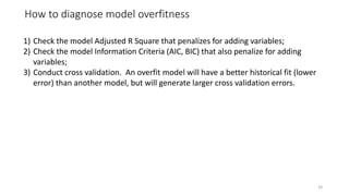
![What is Regularization? … OLS Regression + Penalization
LASSO:
MIN[Sum of Squared Residuals + Lambda(Sum of Absolute Regression Coefficients)]
Ridge Regression:
MIN[Sum of Squared Residuals + Lambda(Sum of Squared Regression Coefficients)]
2](https://image.slidesharecdn.com/regularization-211210001705/85/Regularization-why-you-should-avoid-them-2-320.jpg)
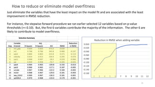
![Showing the OLS term (yellow) vs. Penalization term (orange)
LASSO:
MIN[Sum of Squared Residuals + Lambda(Sum of Absolute Regression Coefficients)]
Ridge Regression:
MIN[Sum of Squared Residuals + Lambda(Sum of Squared Regression Coefficients)]
Lambda is simply a parameter, a value, or a coefficient if you will.
If Lambda = 0, the LASSO or Ridge Regression = OLS Regression
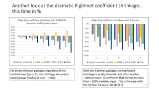
If Lambda is pretty high, the penalization is more severe. And, the variables regression
coefficients will either be zeroed out (LASSO) or very low (Ridge Regression).
3](https://image.slidesharecdn.com/regularization-211210001705/85/Regularization-why-you-should-avoid-them-3-320.jpg)
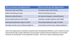
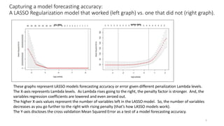
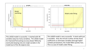
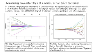
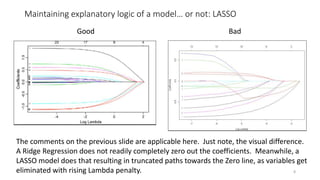
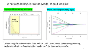
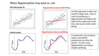

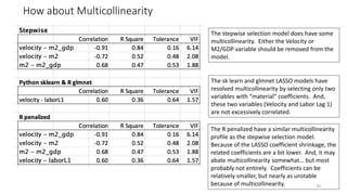
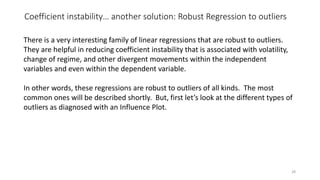


The document discusses the implications of using regularization techniques like Lasso and Ridge regression in statistical modeling, emphasizing their impact on overfitting, underfitting, and variable selection. It highlights how regularization can enhance forecasting accuracy but may compromise the explanatory logic of models by penalizing variable significance. The analysis includes practical examples and critiques of various software applications, concluding that a successful regularization model should improve both accuracy and interpretability.