Download as PDF, PPTX
![5
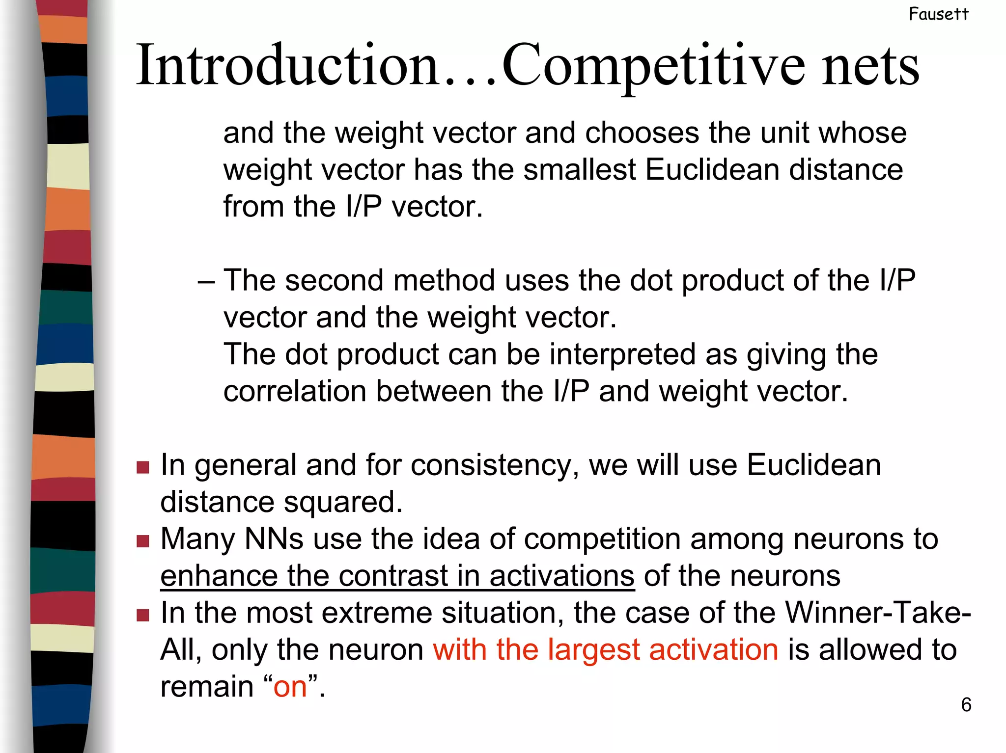
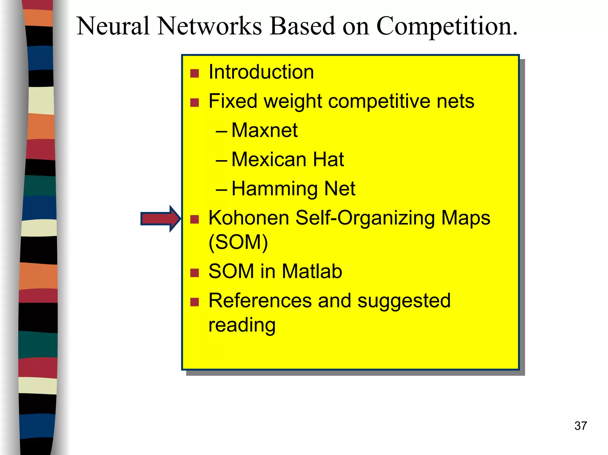
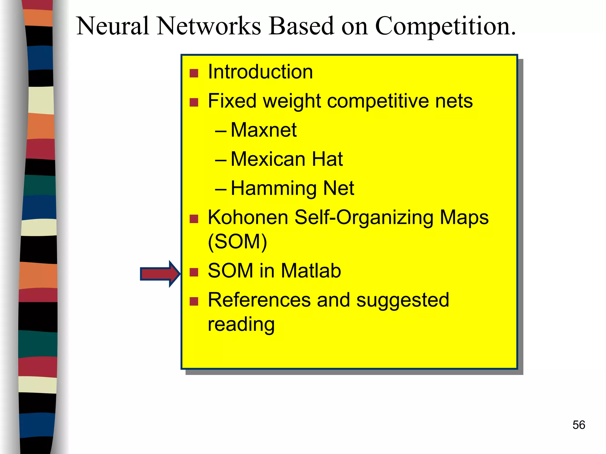
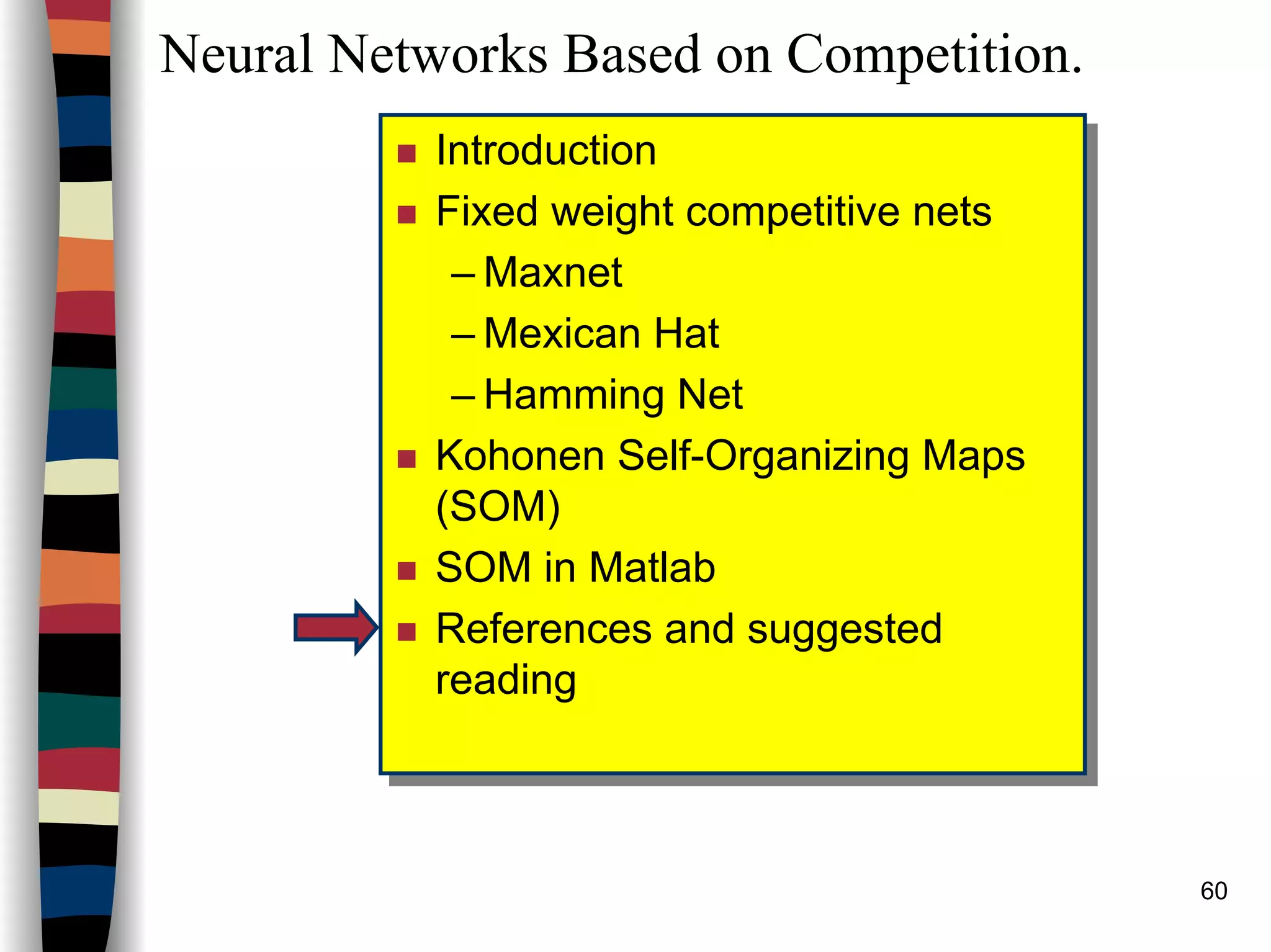
Introduction…Competitive nets
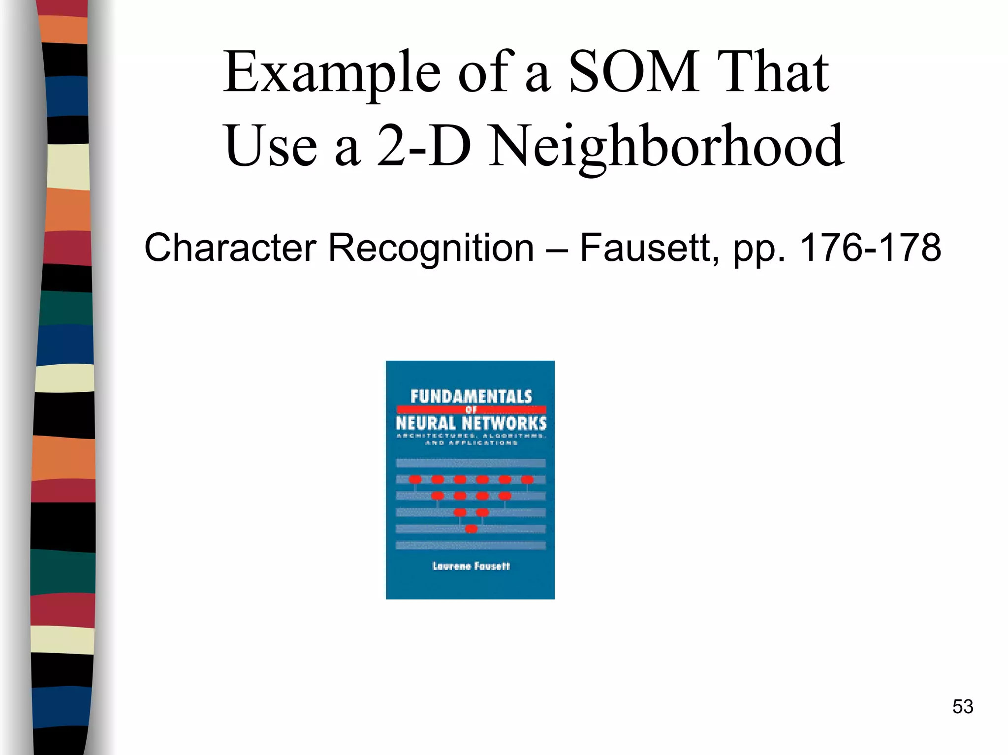
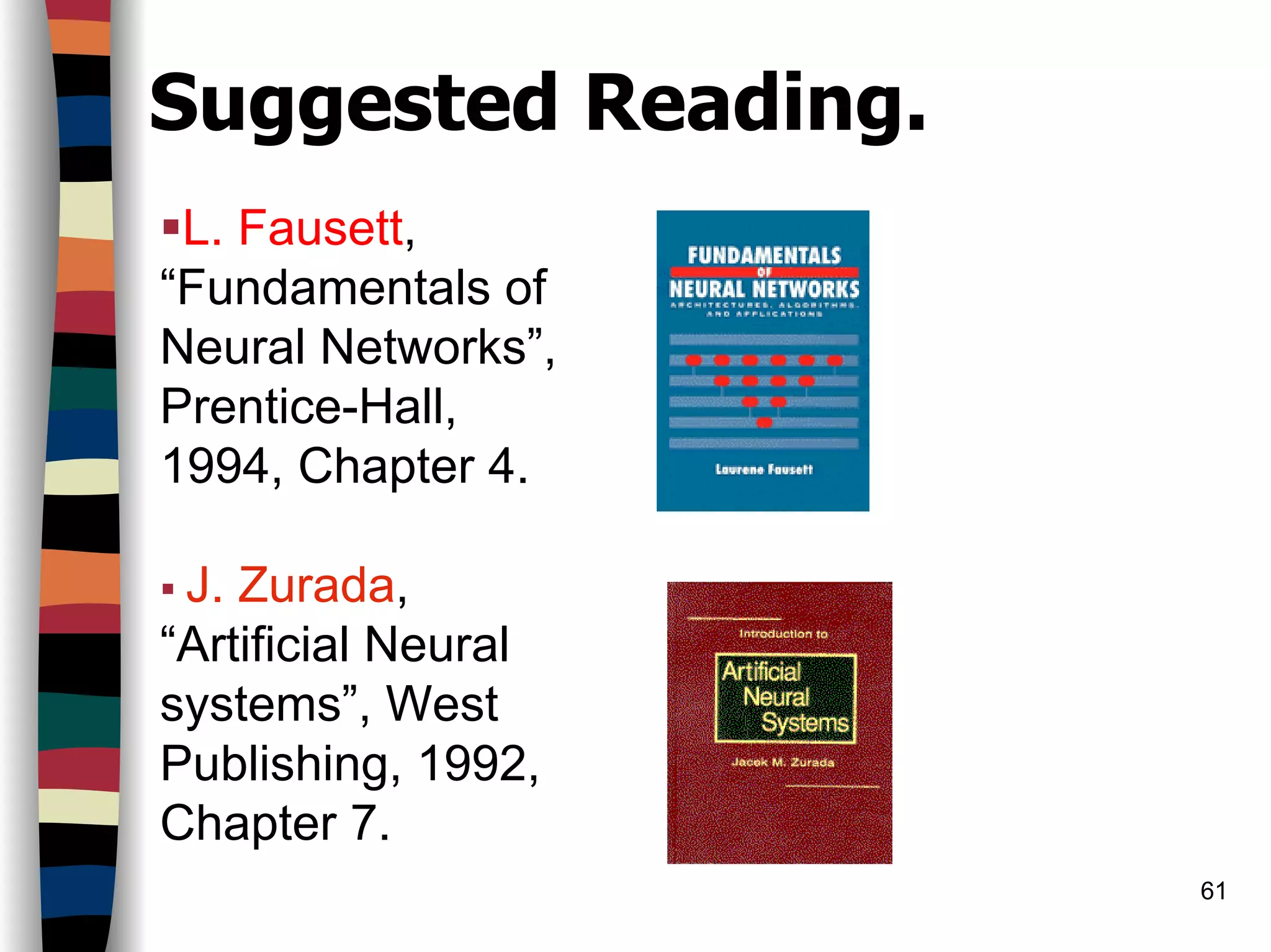
Fausett
The weight update for output (or cluster) unit j is given as:
where x is the input vector, w.j is the weight vector for unit j,
and α the learning rate, decreases as learning proceeds.
Two methods of determining the closest weight vector to a
pattern vector are commonly used for self-organizing nets.
Both are based on the assumption that the weight vector
for each cluster (output) unit serves as an exemplar for the
input vectors that have been assigned to that unit during
learning.
– The first method of determining the winner uses the
squared Euclidean distance between the I/P vector
[ ]
old)()1(
old)()old()new(
.
...
j
jjj
wx
wxww
αα
α
−+
−+=](https://image.slidesharecdn.com/lect7-uwa-160515045203/75/Artificial-Neural-Networks-Lect7-Neural-networks-based-on-competition-5-2048.jpg)
![10
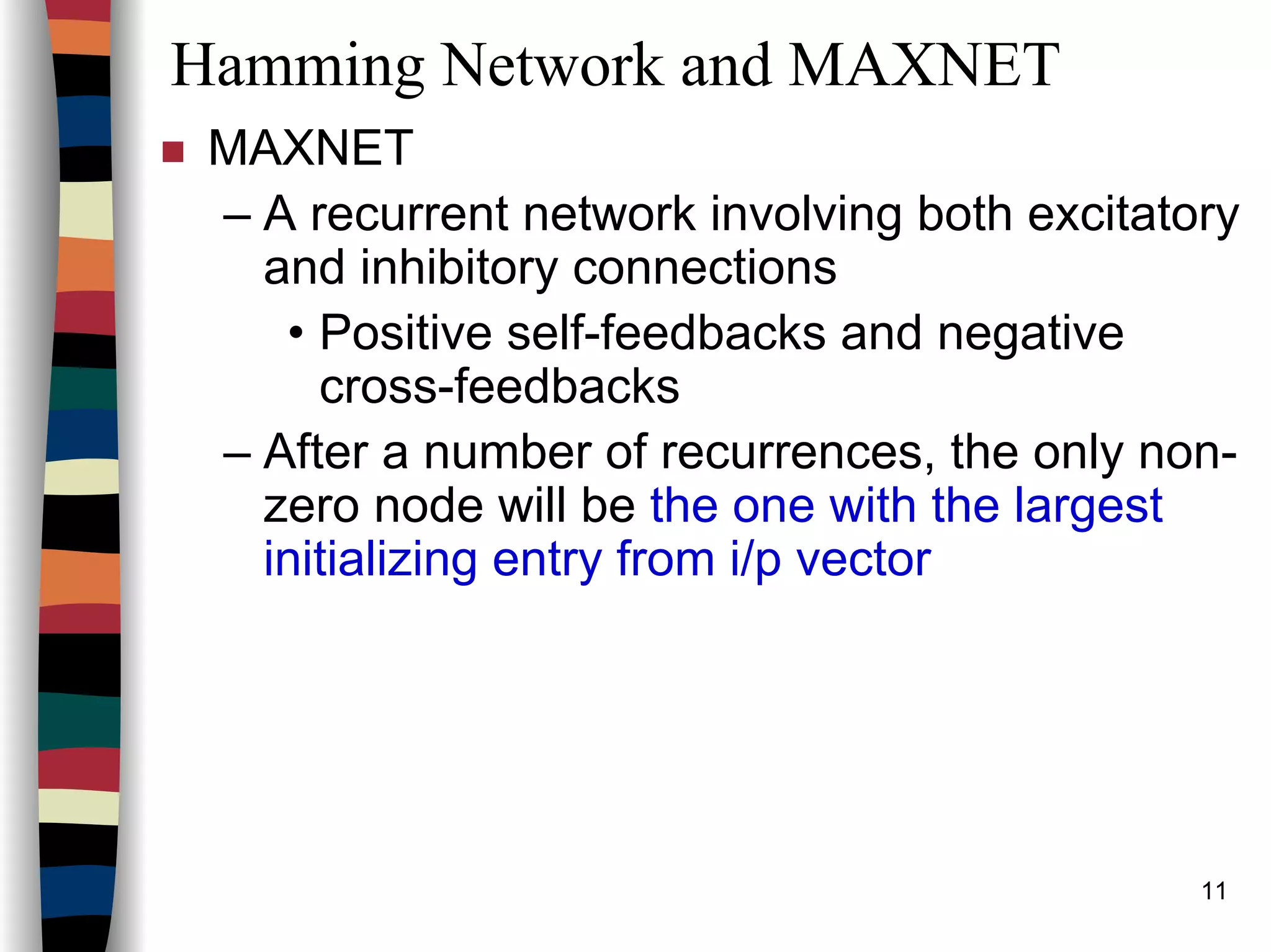
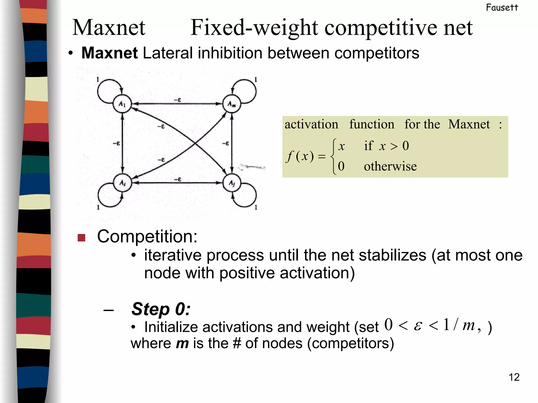
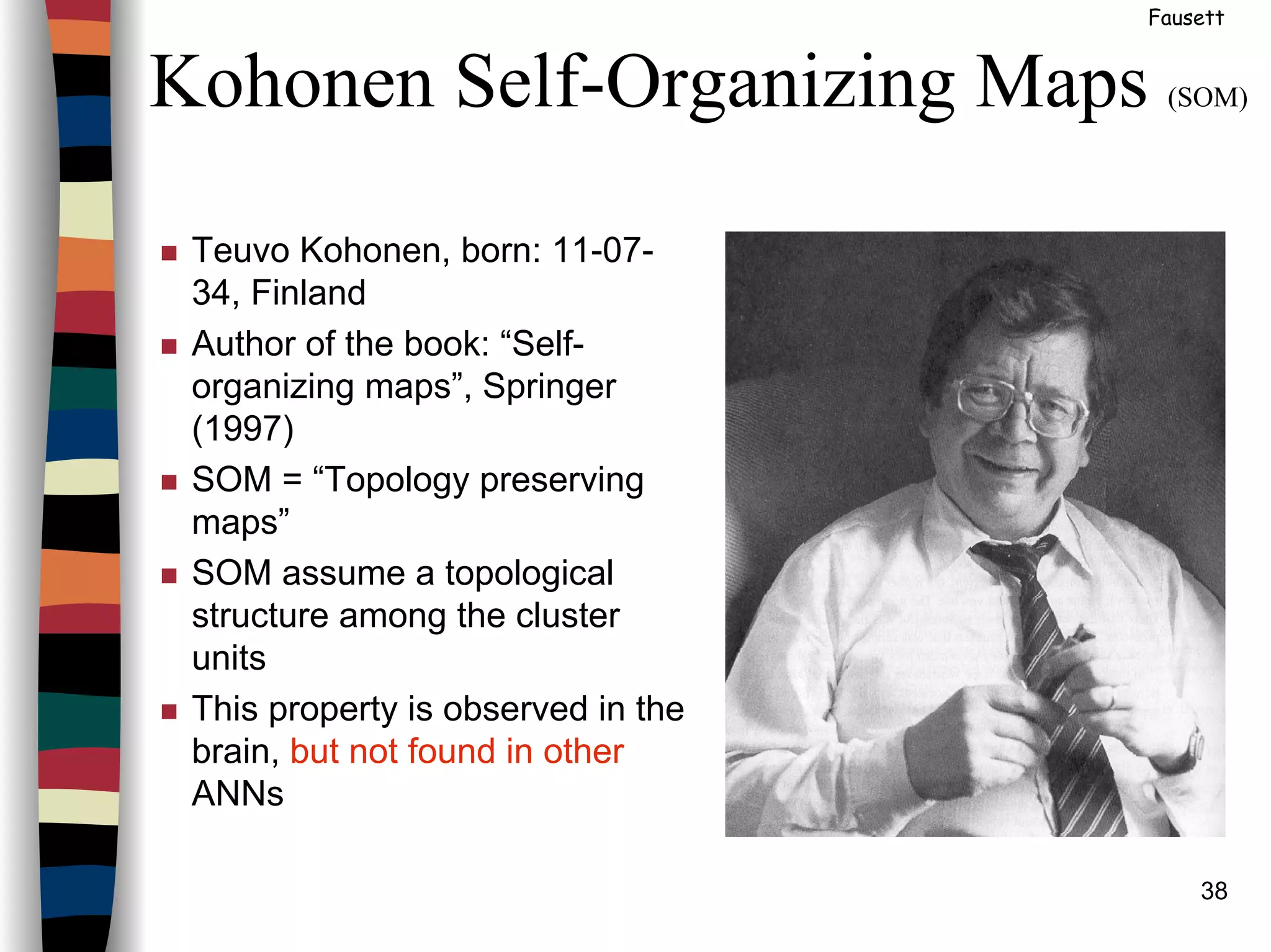
MAXNET
[ ]k
M
k
yWy Γ=+1
−−
−−
−−
=
1..
.
.
..1
..1
εε
εε
εε
MW
( )
≥
<
=
0,
0,0
netnet
net
netf
p
10 << ε](https://image.slidesharecdn.com/lect7-uwa-160515045203/75/Artificial-Neural-Networks-Lect7-Neural-networks-based-on-competition-10-2048.jpg)
![14
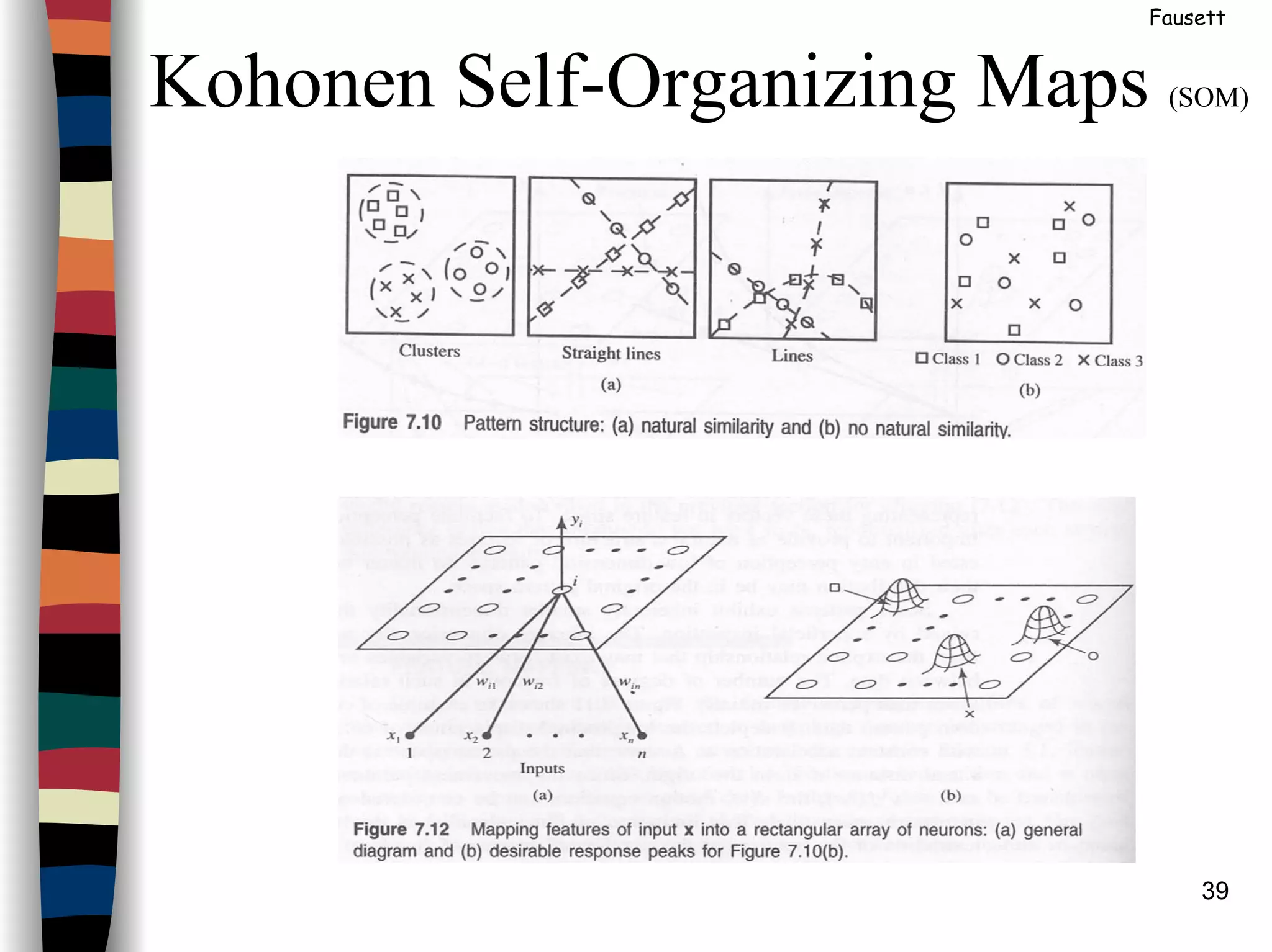
Example
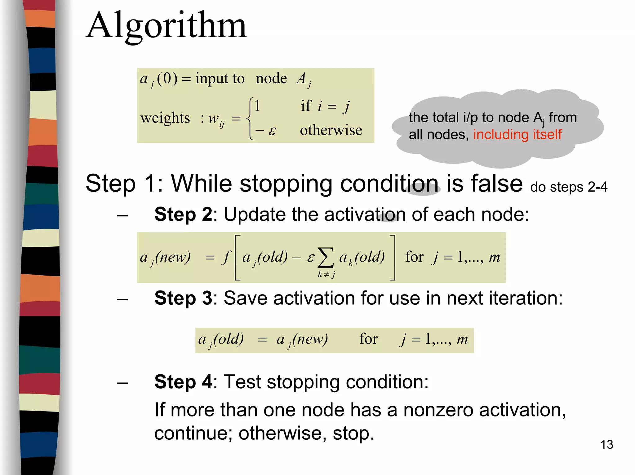
Note that in step 2, the i/p to the function f is the total
i/p to node Aj from all nodes, including itself.
Some precautions should be incorporated to handle
the situation in which two or more units have the
same, maximal, input.
Example:
ε = .2 and the initial activations (input signals) are:
a1(0) = .2, a2(0) = .4 a3(0) = .4 a4(0) = .8
As the net iterates, the activations are:
a1(1) = f{a1(0) -.2 [a2(0) + a3(0) + a4(0)]} = f(-.12)=0
a1(1) = .0, a2(1) = .08 a3(1) = .32 a4(1) = .56
a1(2) = .0, a2(2) = .0 a3(2) = .192 a4(2) = .48
a1(3) = .0, a2(3) = .0 a3(3) = .096 a4(3) = .442
a1(4) = .0, a2(4) = .0 a3(4) = .008 a4(4) = .422
a1(5) = .0, a2(5) = .0 a3(5) = .0 a4(5) = .421
The only node
to remain on](https://image.slidesharecdn.com/lect7-uwa-160515045203/75/Artificial-Neural-Networks-Lect7-Neural-networks-based-on-competition-14-2048.jpg)
![32
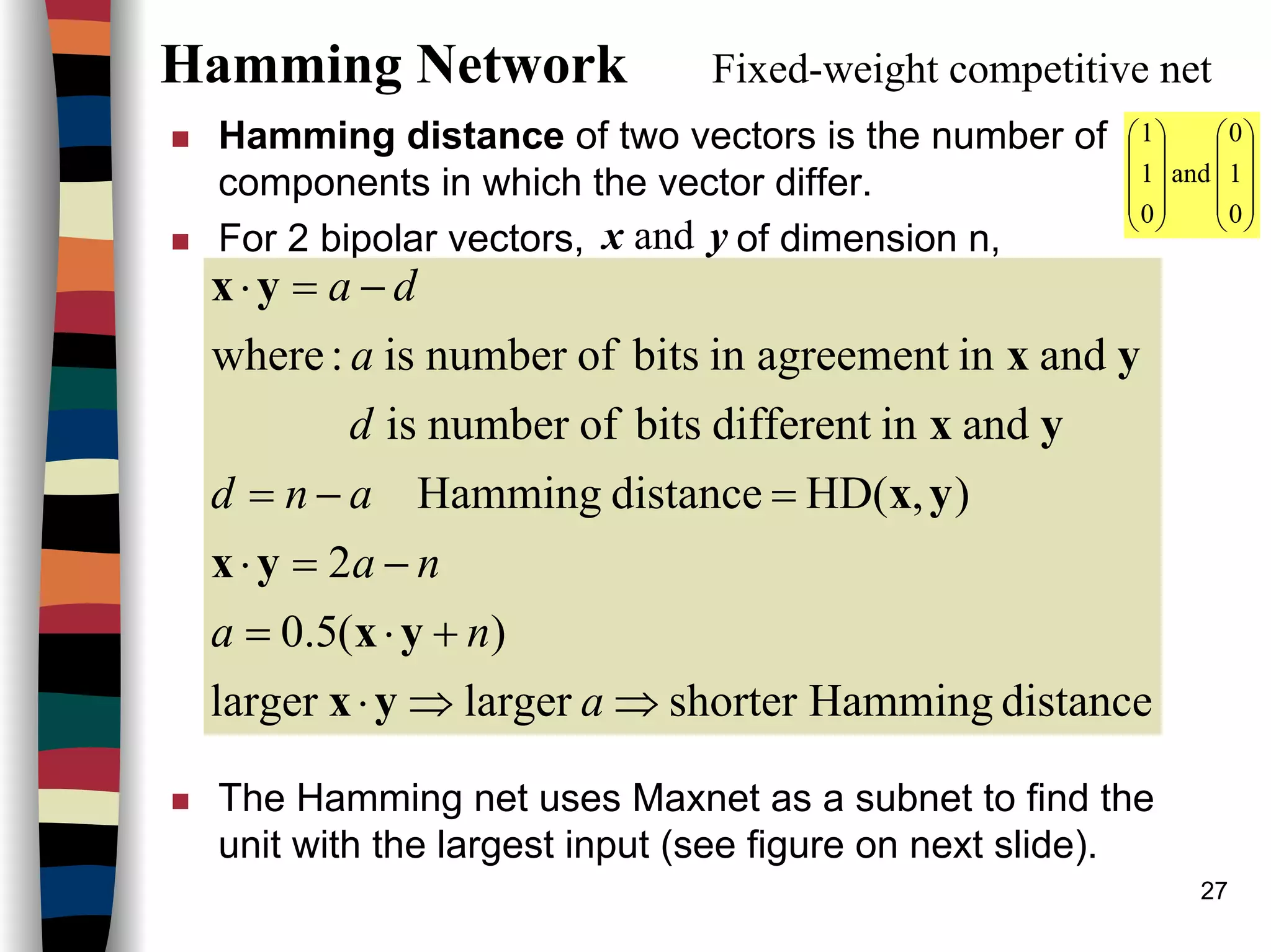
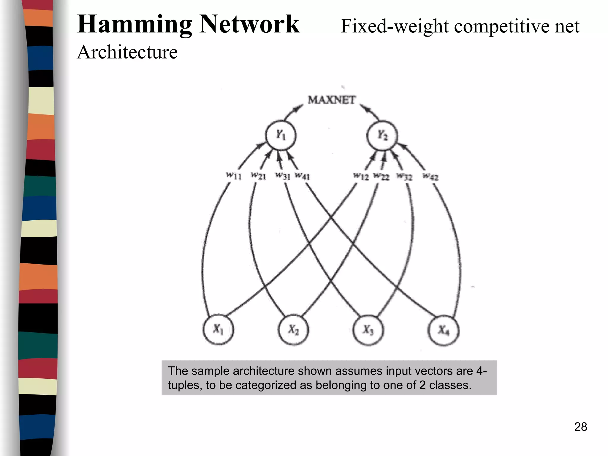
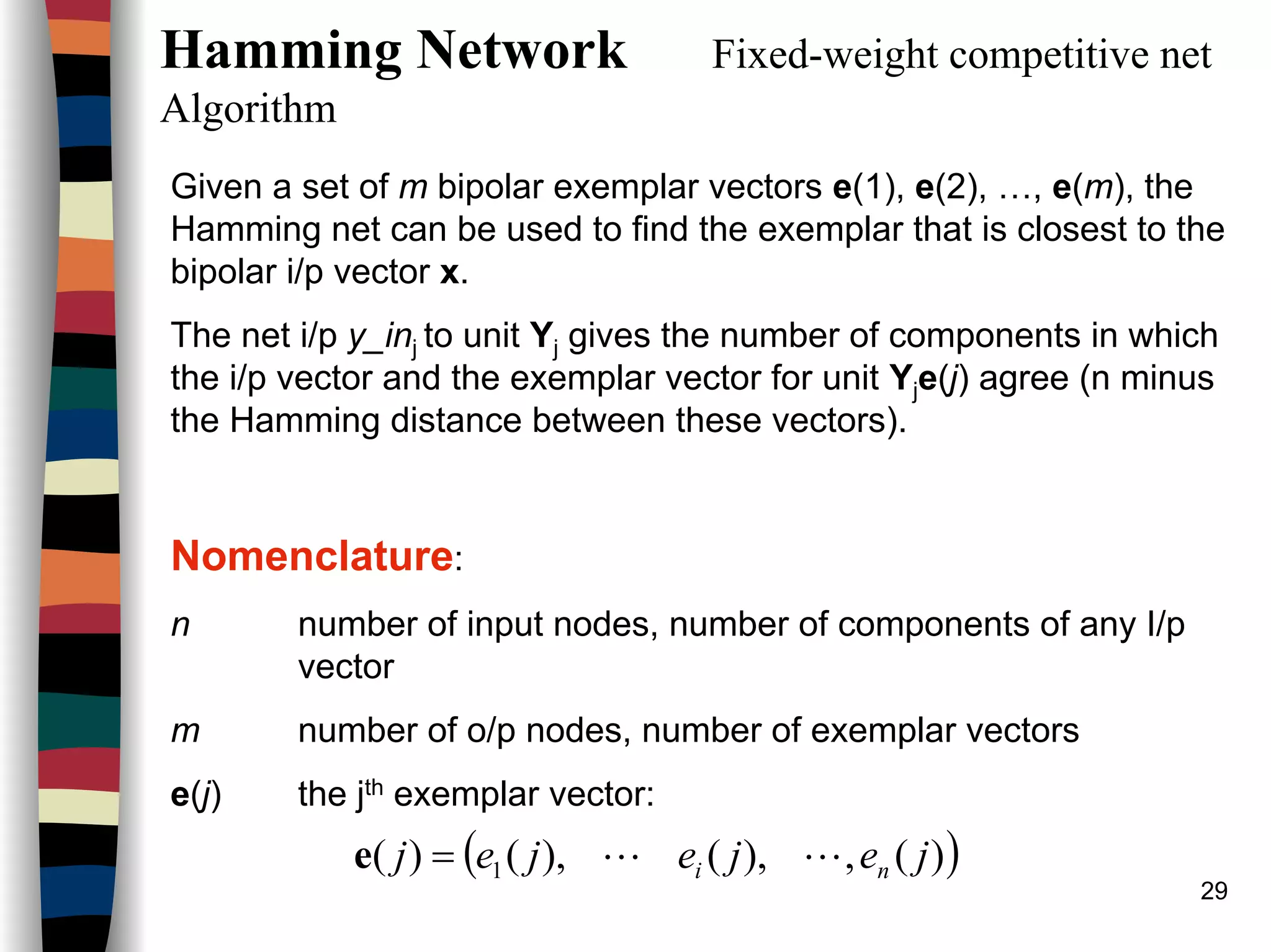
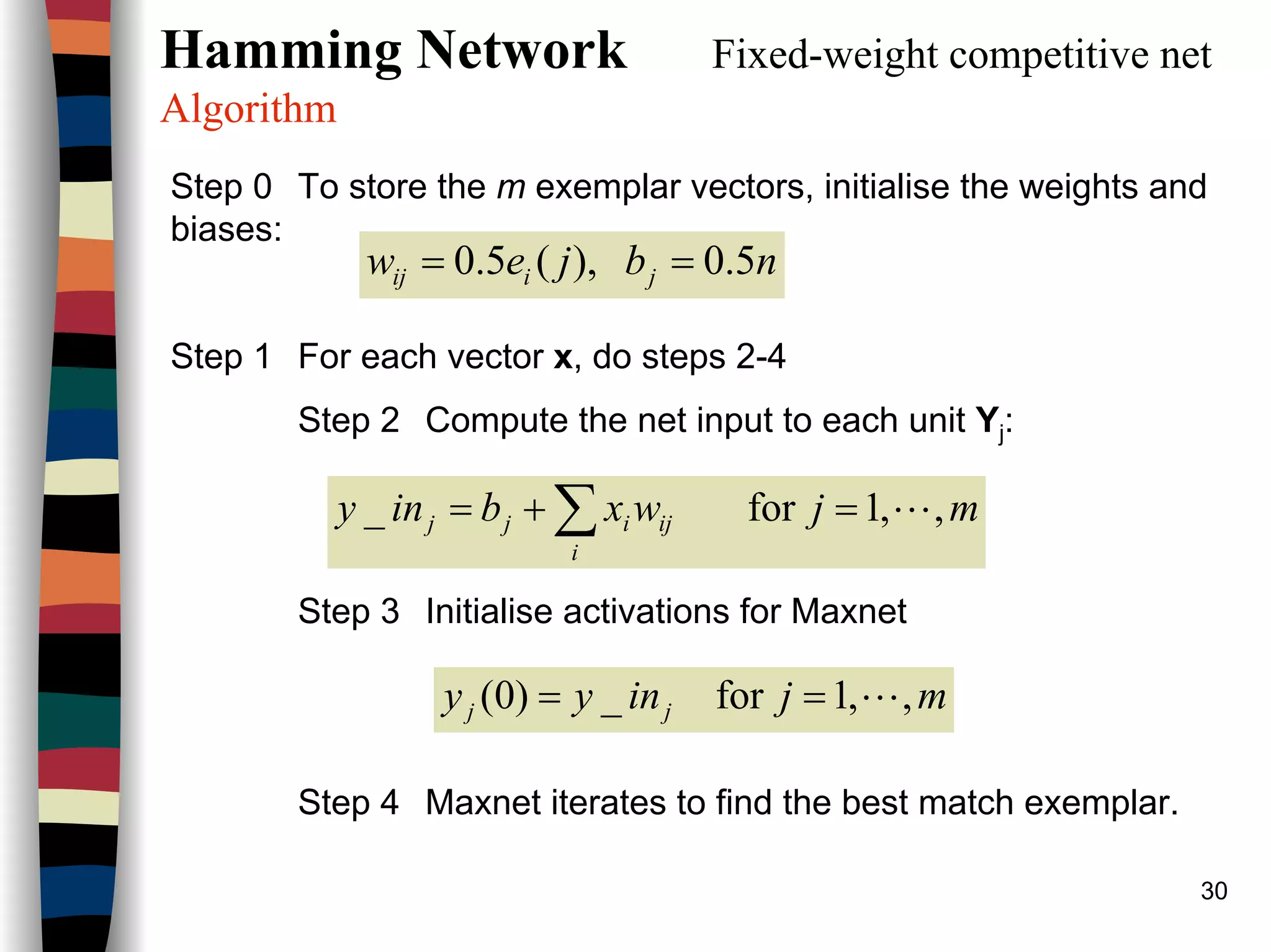
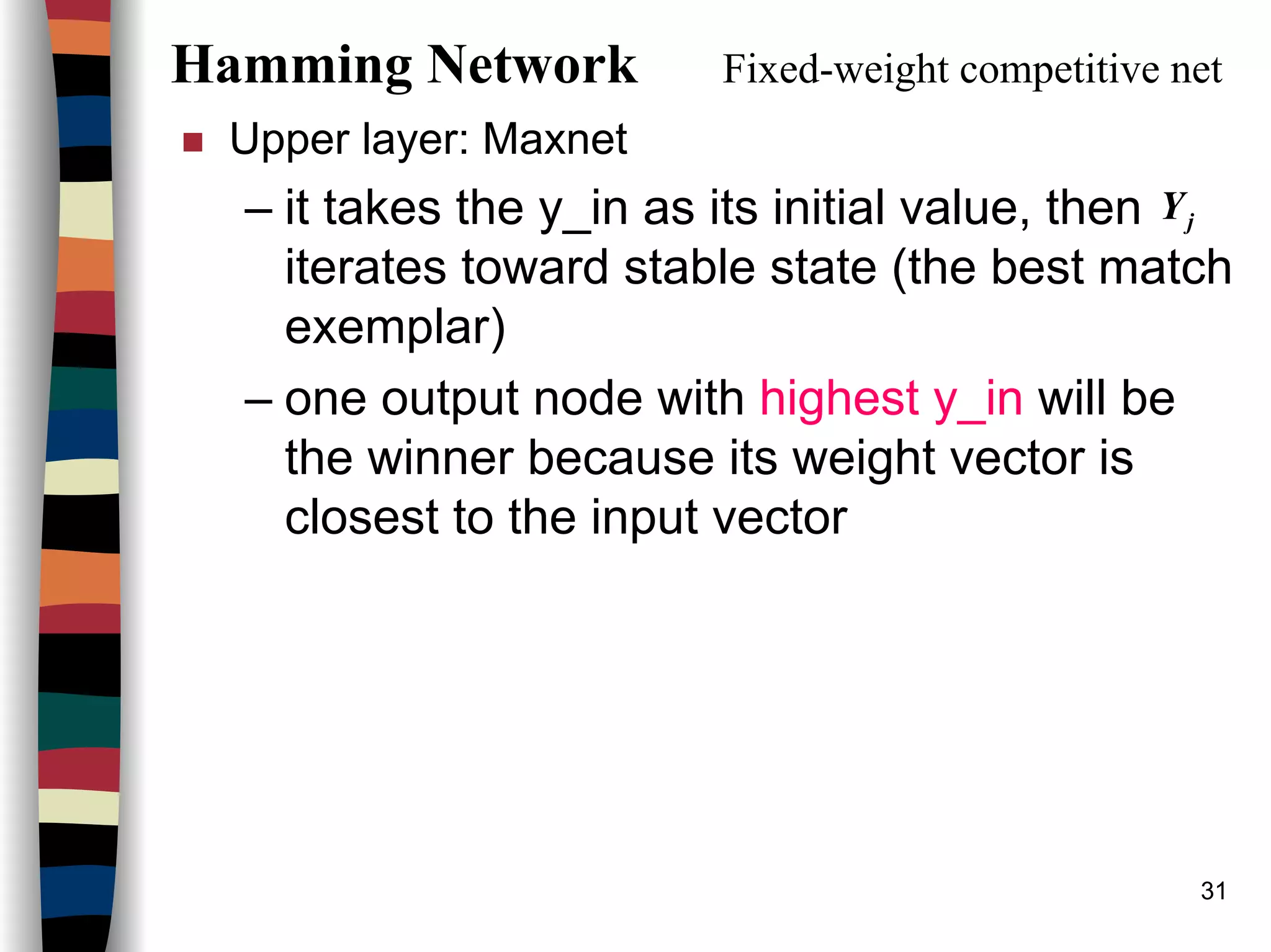
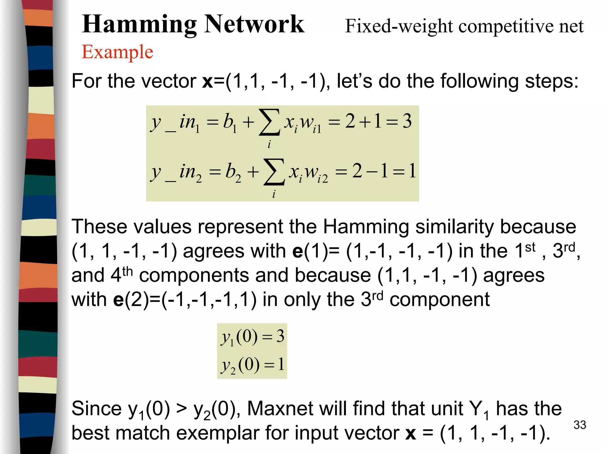
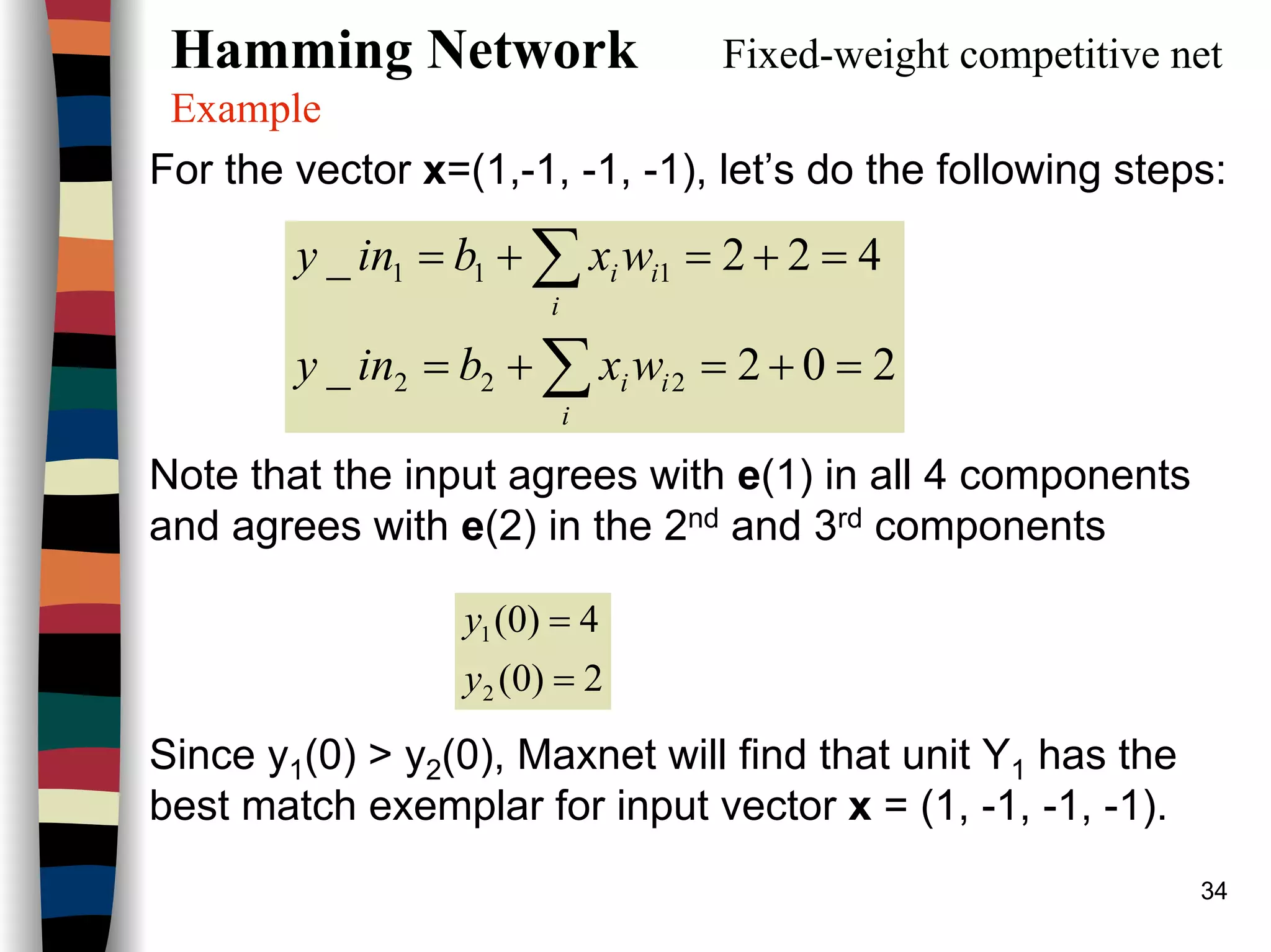
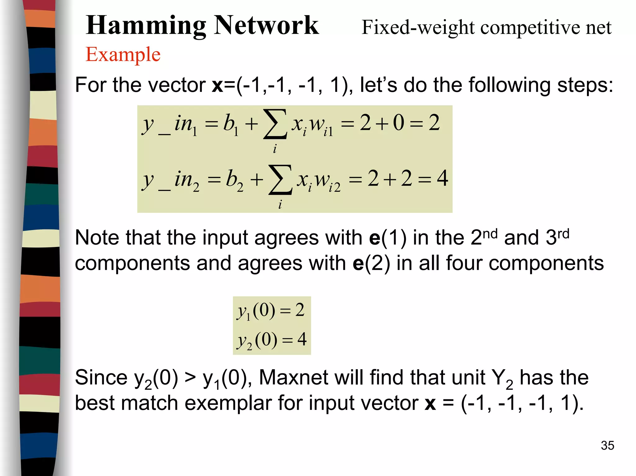
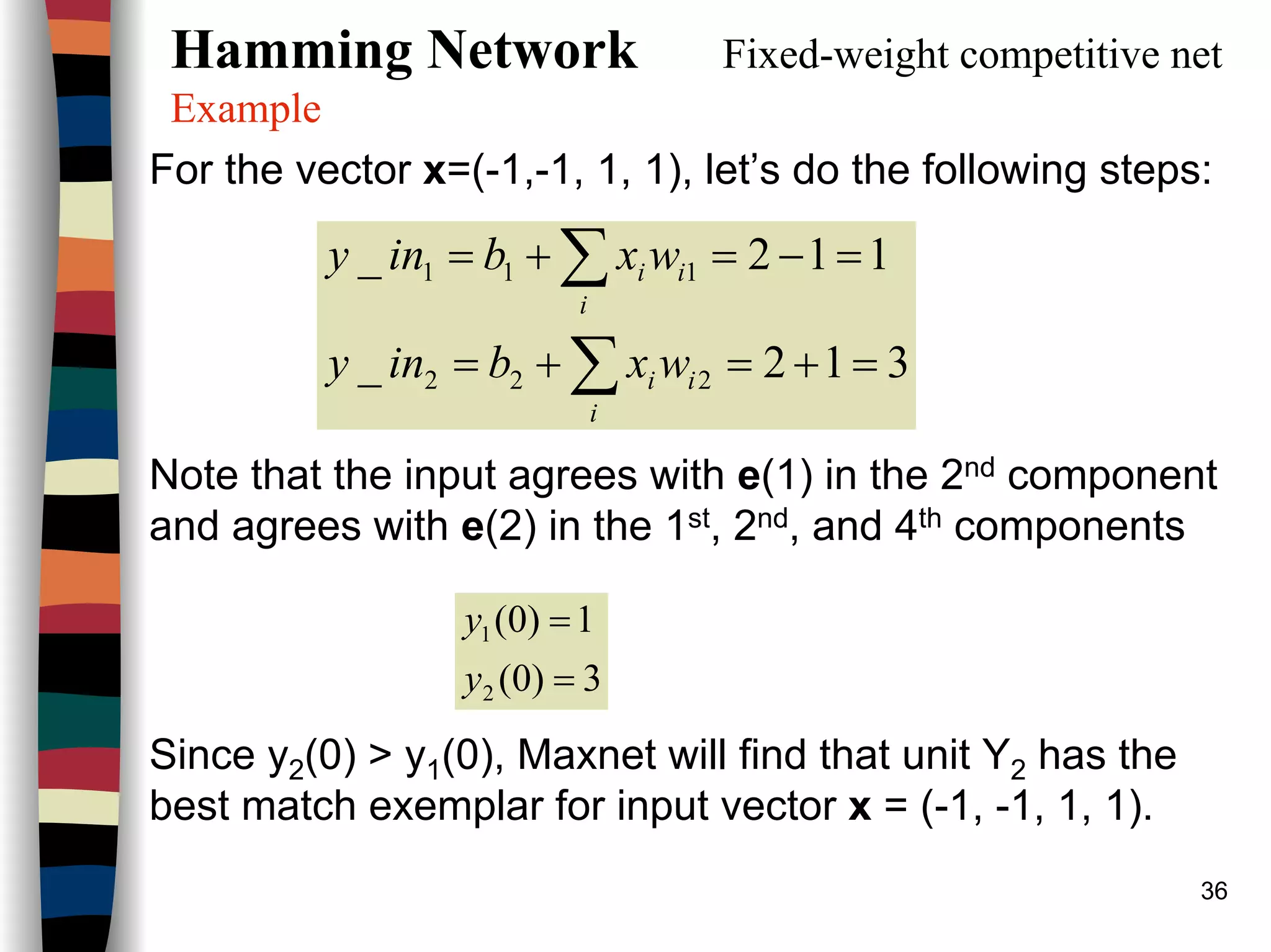
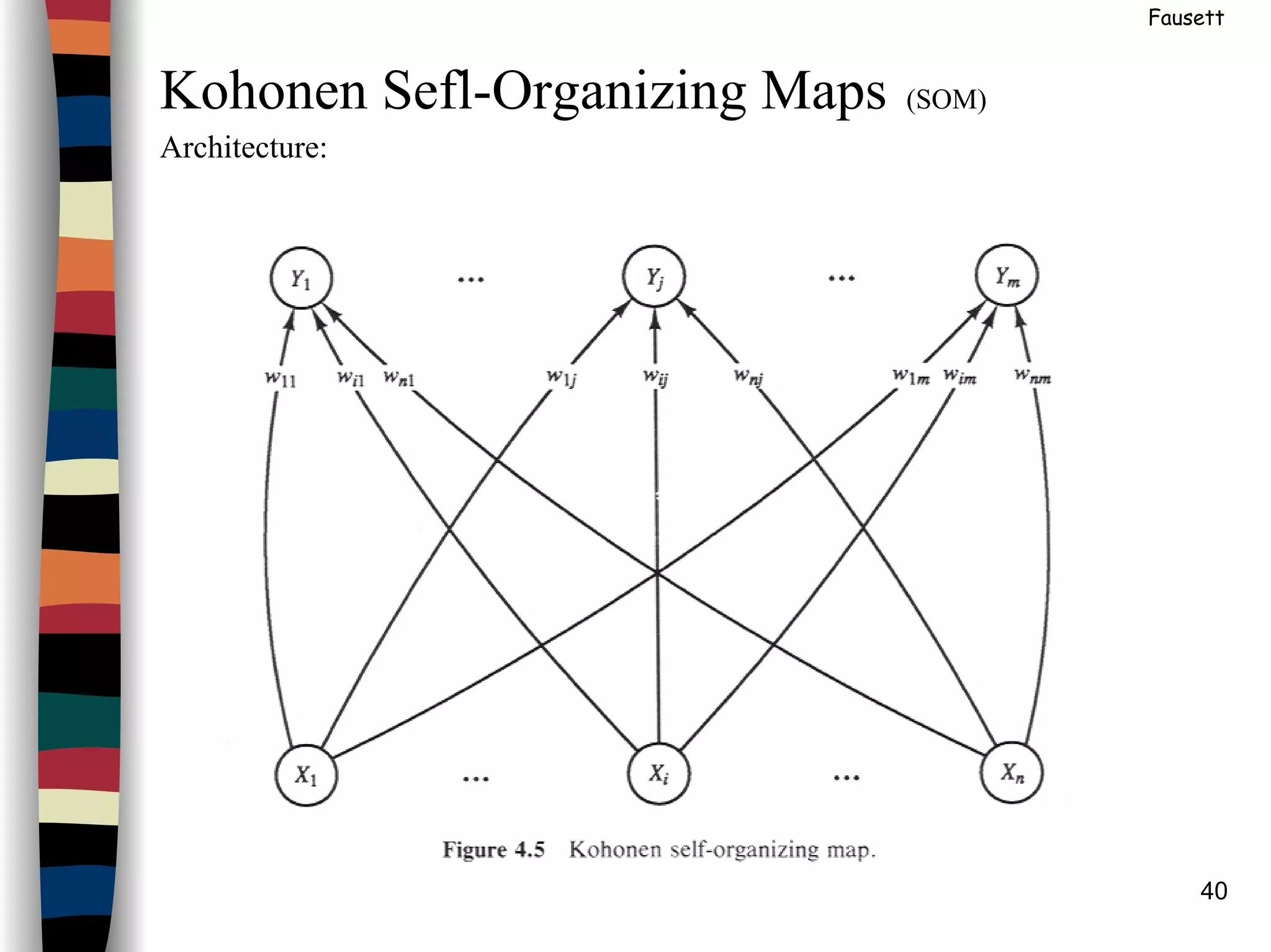
Hamming Network Fixed-weight competitive net
Example (see architecture n=4)
[ ]
[ ] patterns)(exemplar2casein thism1-1,-1,-1,)2(
1-1,-1,-1,)1(
:ectorsexemplar vGiven the
=−=
=
e
e
The Hamming net can be used to find the exemplar that is closest to each of the
bipolar i/p patterns, (1, 1, -1, -1), (1, -1, -1, -1), (-1, -1, -1, 1), and (-1, -1, 1, 1)
Step 1: Store the m exemplar vectors in the weights:
case)(in this4nodesinputofnumber
2/2
:biasestheInitialize
2
)(
rewhe
5.5.
5.5.
5.5.
5.5.
21
==
===
=
−−
−−
−−
−
=
n
nbb
je
wW i
ij](https://image.slidesharecdn.com/lect7-uwa-160515045203/75/Artificial-Neural-Networks-Lect7-Neural-networks-based-on-competition-32-2048.jpg)
![41
Fausett
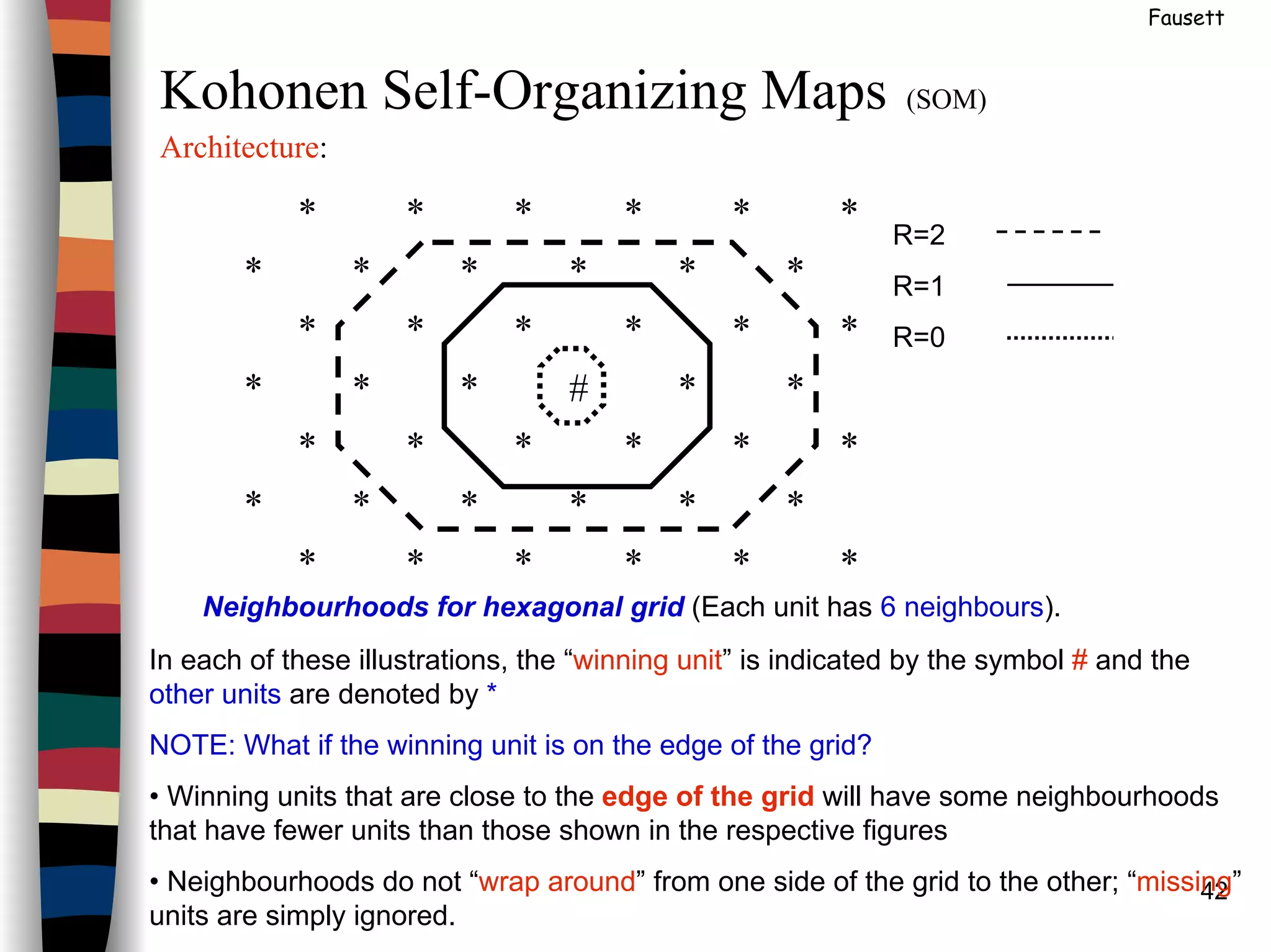
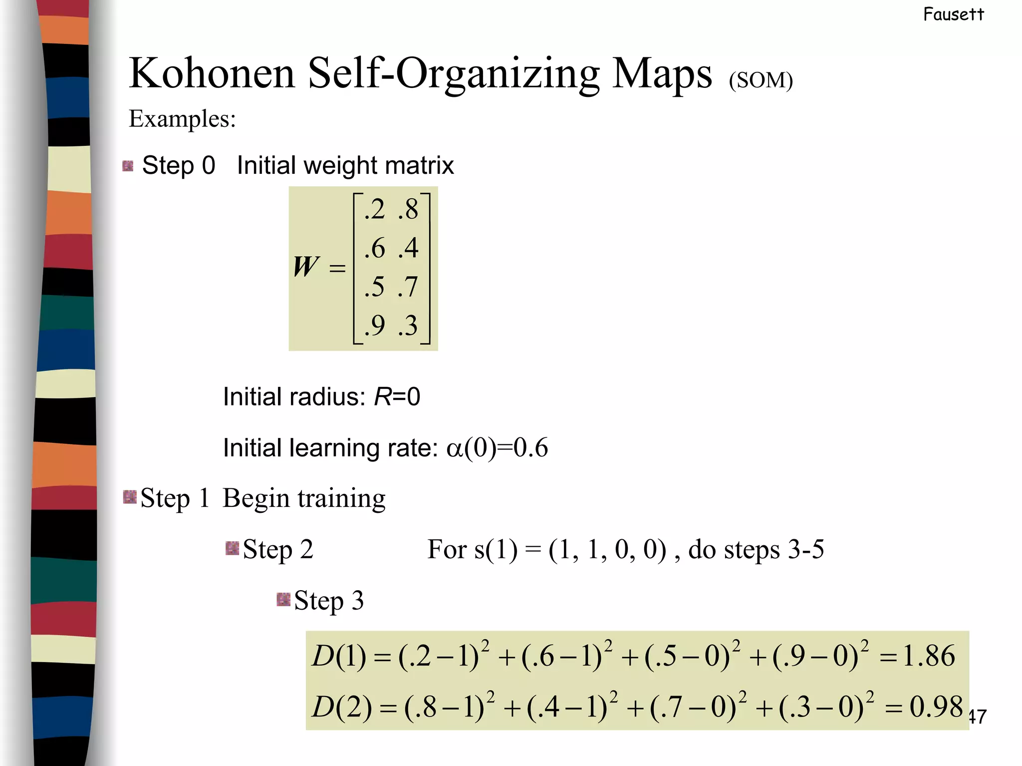
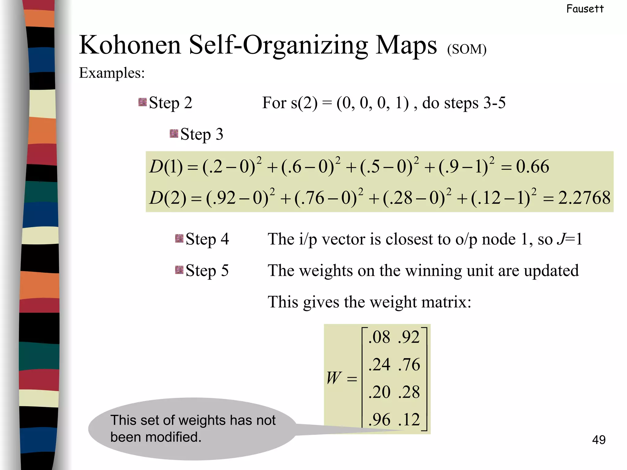
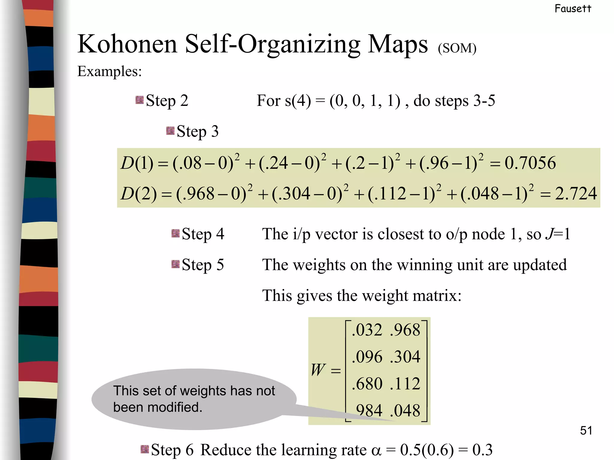
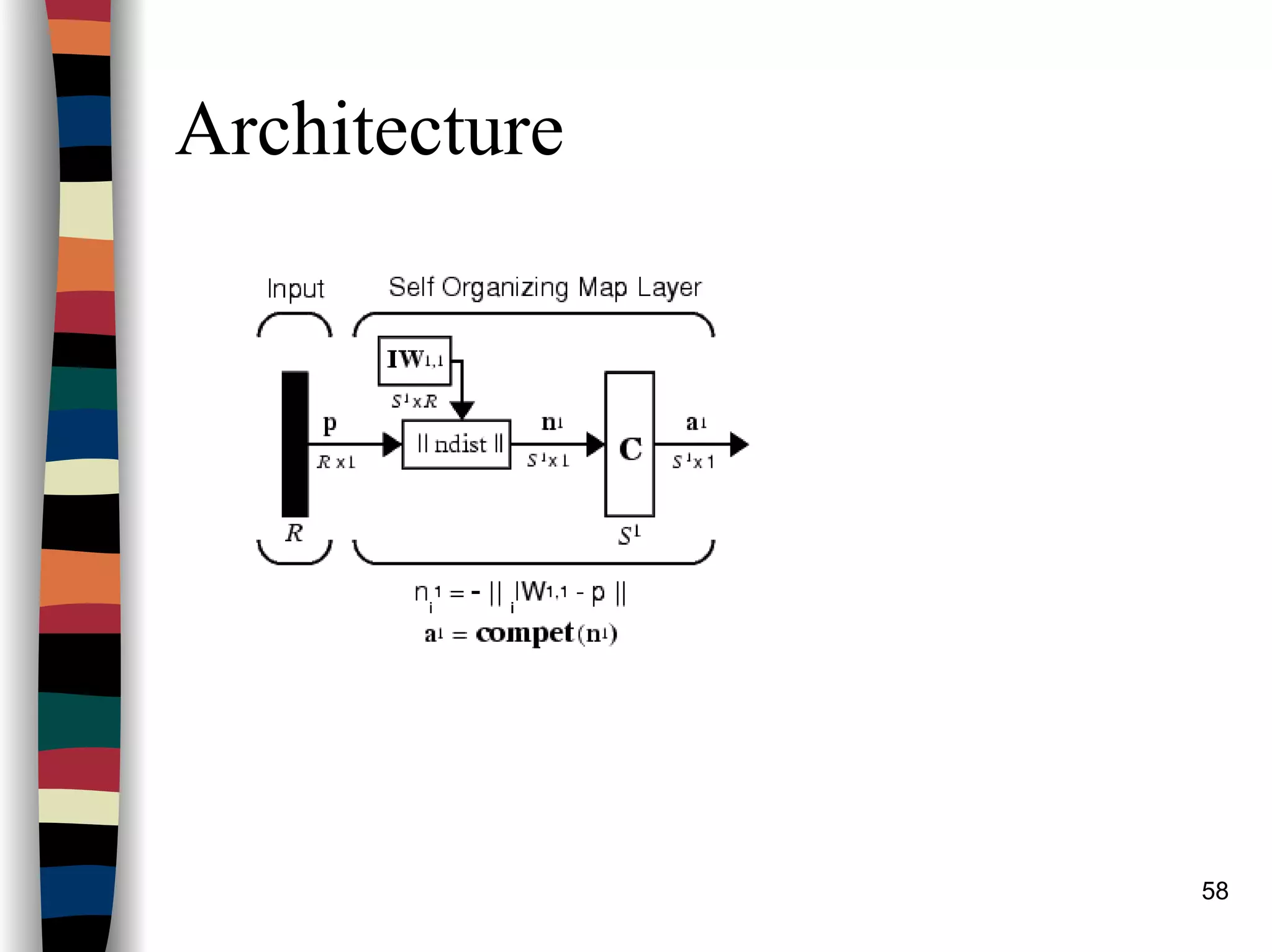
Kohonen Self-Organizing Maps (SOM)
Architecture:
* * {* (* [#] *) *} * *
{ } R=2 ( ) R=1 [ ] R=0
Linear array of cluster units
This figure represents the neighborhood of the unit designated by # in a 1D topology
(with 10 cluster units).
*******
*******
*******
***#***
*******
*******
*******
R=2
R=1
R=0
Neighbourhoods for rectangular grid (Each unit has 8 neighbours)](https://image.slidesharecdn.com/lect7-uwa-160515045203/75/Artificial-Neural-Networks-Lect7-Neural-networks-based-on-competition-41-2048.jpg)
()( oldwxoldwneww ijiijij −+= α](https://image.slidesharecdn.com/lect7-uwa-160515045203/75/Artificial-Neural-Networks-Lect7-Neural-networks-based-on-competition-44-2048.jpg)
()(
2
222
+
−+=
This set of weights has not
been modified.
=
12.9.
28.5.
76.6.
92.2.
W](https://image.slidesharecdn.com/lect7-uwa-160515045203/75/Artificial-Neural-Networks-Lect7-Neural-networks-based-on-competition-48-2048.jpg)
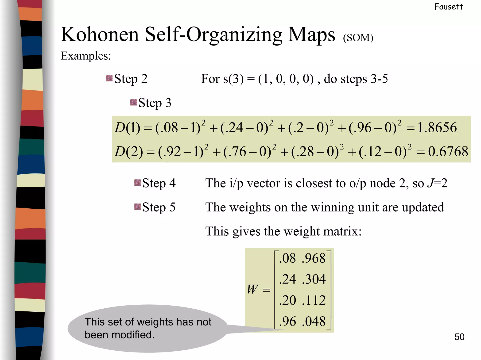
()(
+
−+=
=
024.999.
055.630.
360.047.
980.016.
W
=
0.00.1
0.05.
5.00.
0.10.
W
The 1st
column is the average
of the 2 vects in cluster 1, and
the 2nd
col is the average of
the 2 vects in cluster 2
This set of weights has not
been modified.](https://image.slidesharecdn.com/lect7-uwa-160515045203/75/Artificial-Neural-Networks-Lect7-Neural-networks-based-on-competition-52-2048.jpg)

![59
CreatingaSOM
newsom -- Create a self-organizing map
Syntax
net = newsom
net = newsom(PR,[D1,D2,...],TFCN,DFCN,OLR,OSTEPS,TLR,TND)
Description
net = newsom creates a new network with a dialog box.
net = newsom (PR,[D1,D2,...],TFCN,DFCN,OLR,OSTEPS,TLR,TND)
takes,
PR - R x 2 matrix of min and max values for R input elements.
Di - Size of ith layer dimension, defaults = [5 8].
TFCN - Topology function, default ='hextop'.
DFCN - Distance function, default ='linkdist'.
OLR - Ordering phase learning rate, default = 0.9.
OSTEPS - Ordering phase steps, default = 1000.
TLR - Tuning phase learning rate, default = 0.02;
TND - Tuning phase neighborhood distance, default = 1.
and returns a new self-organizing map.
The topology function TFCN can be hextop, gridtop, or randtop. The
distance function can be linkdist, dist, or mandist.](https://image.slidesharecdn.com/lect7-uwa-160515045203/75/Artificial-Neural-Networks-Lect7-Neural-networks-based-on-competition-59-2048.jpg)

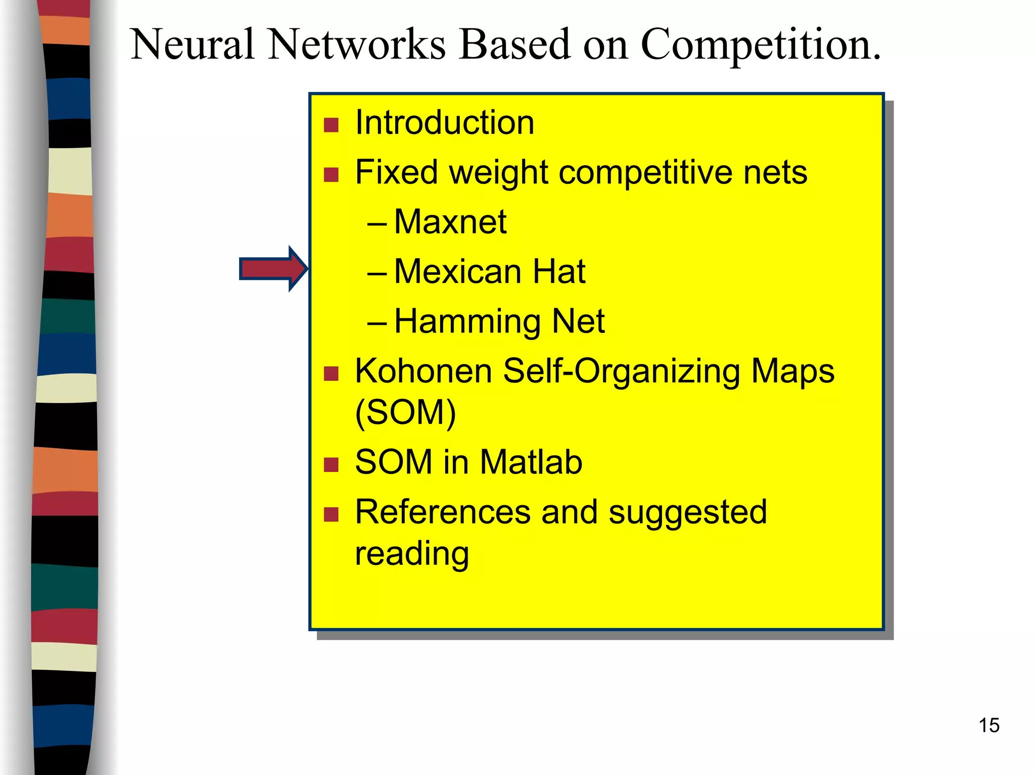
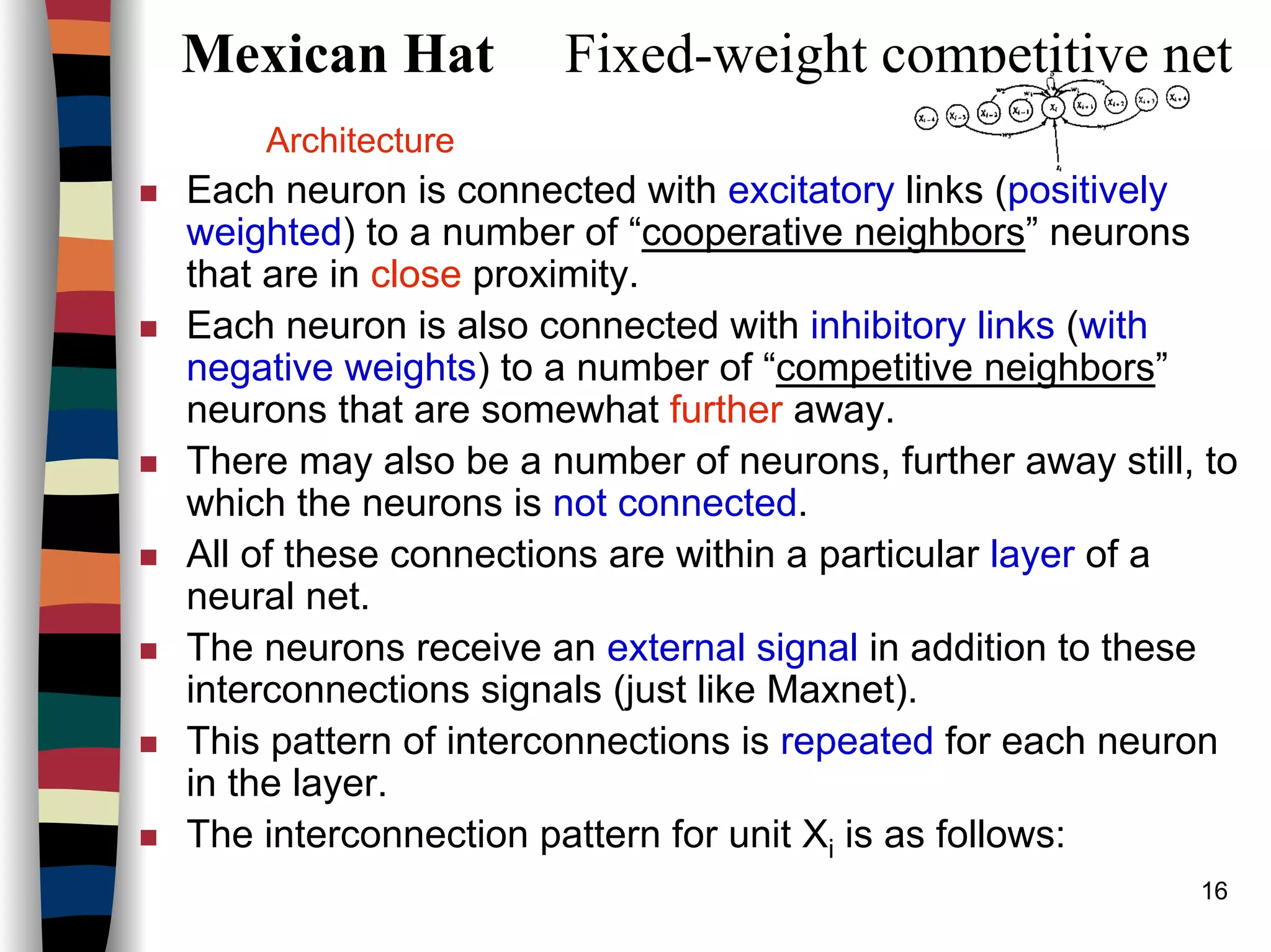
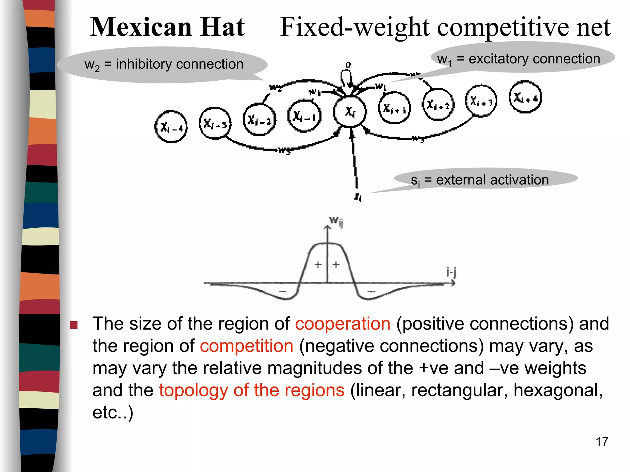
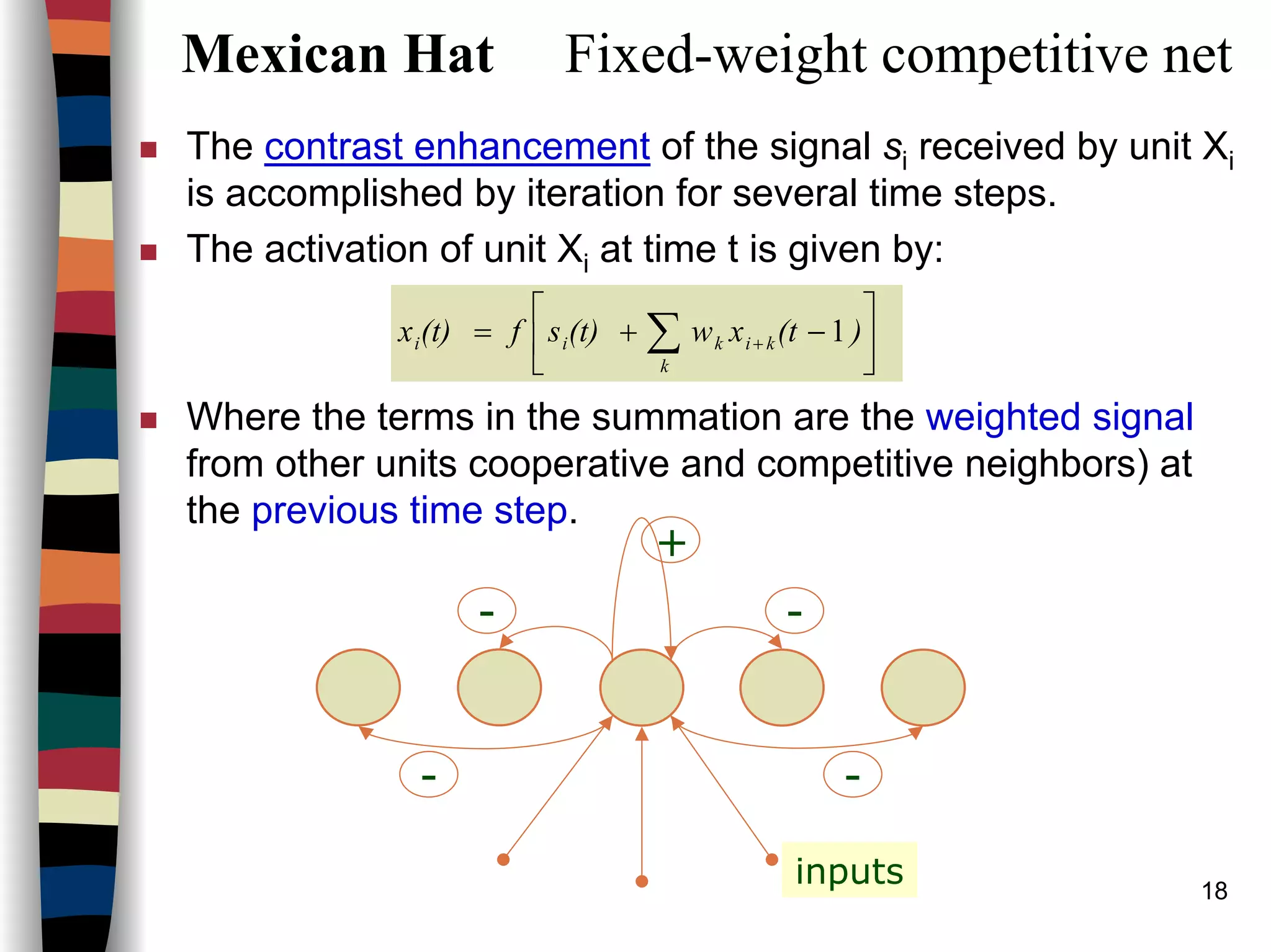
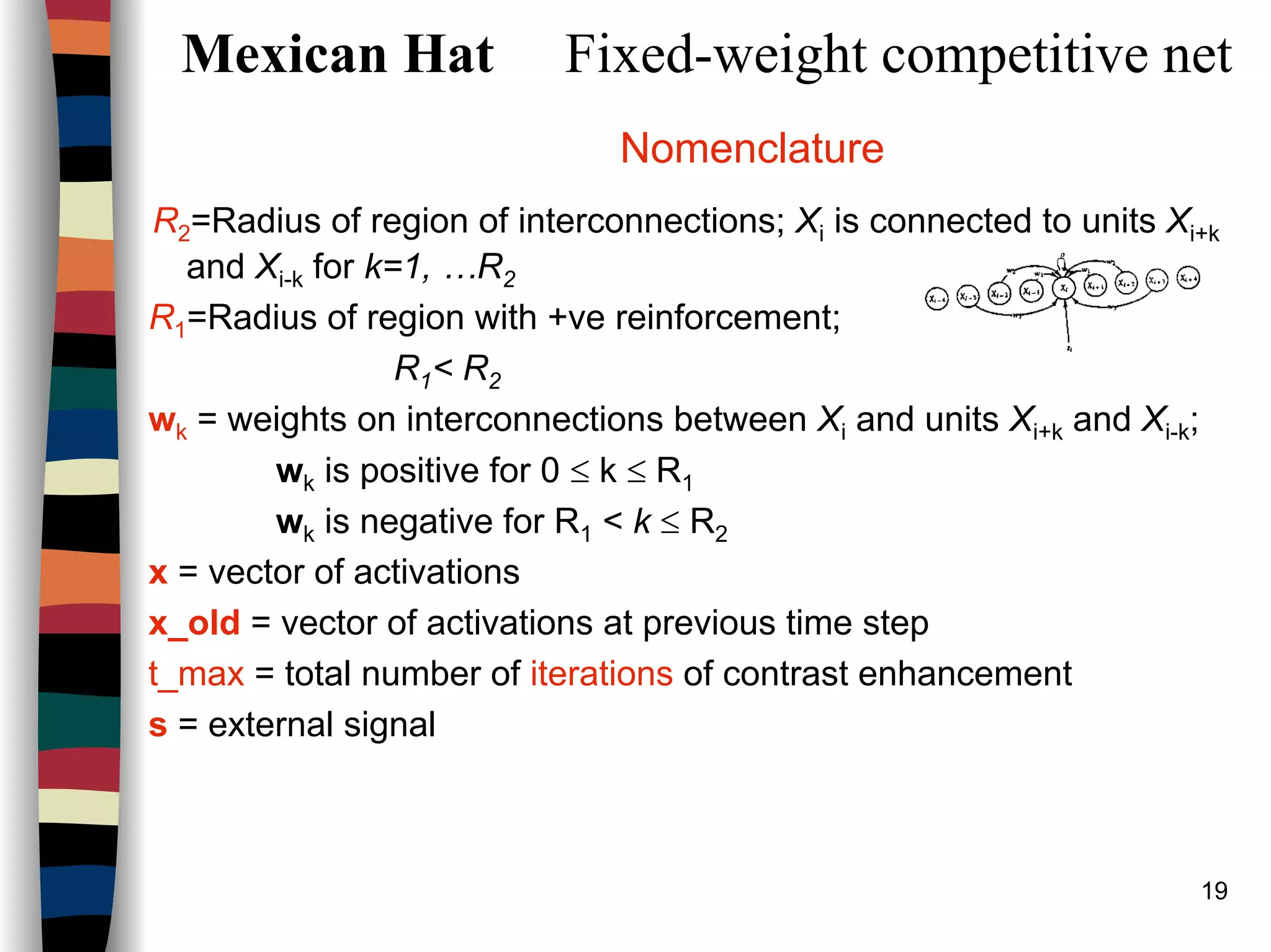
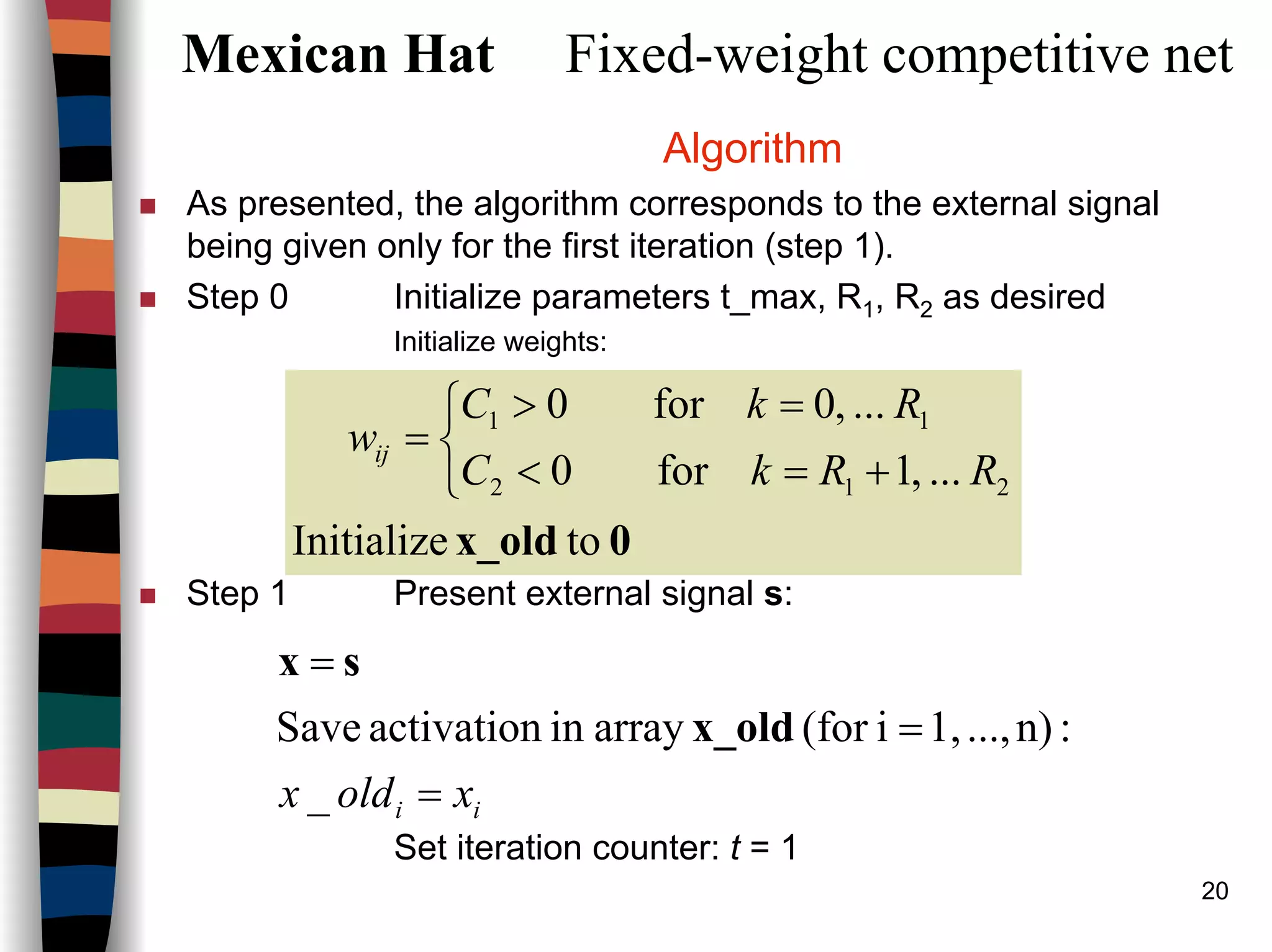
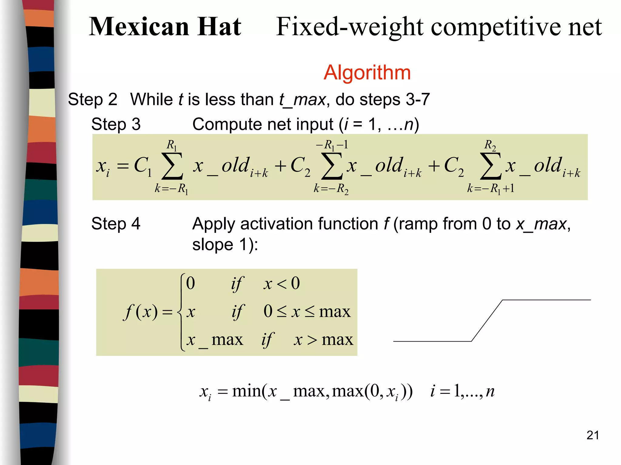
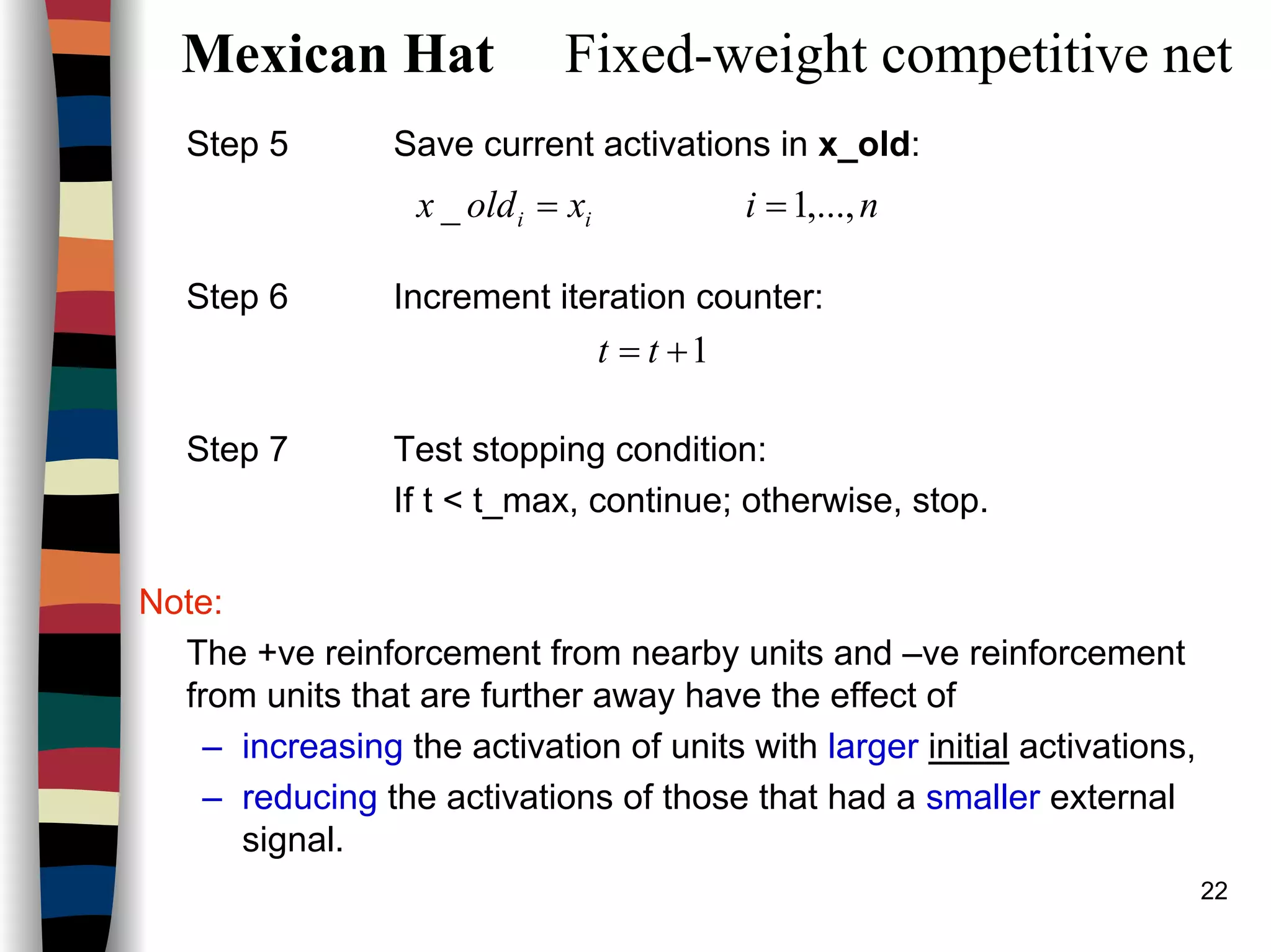
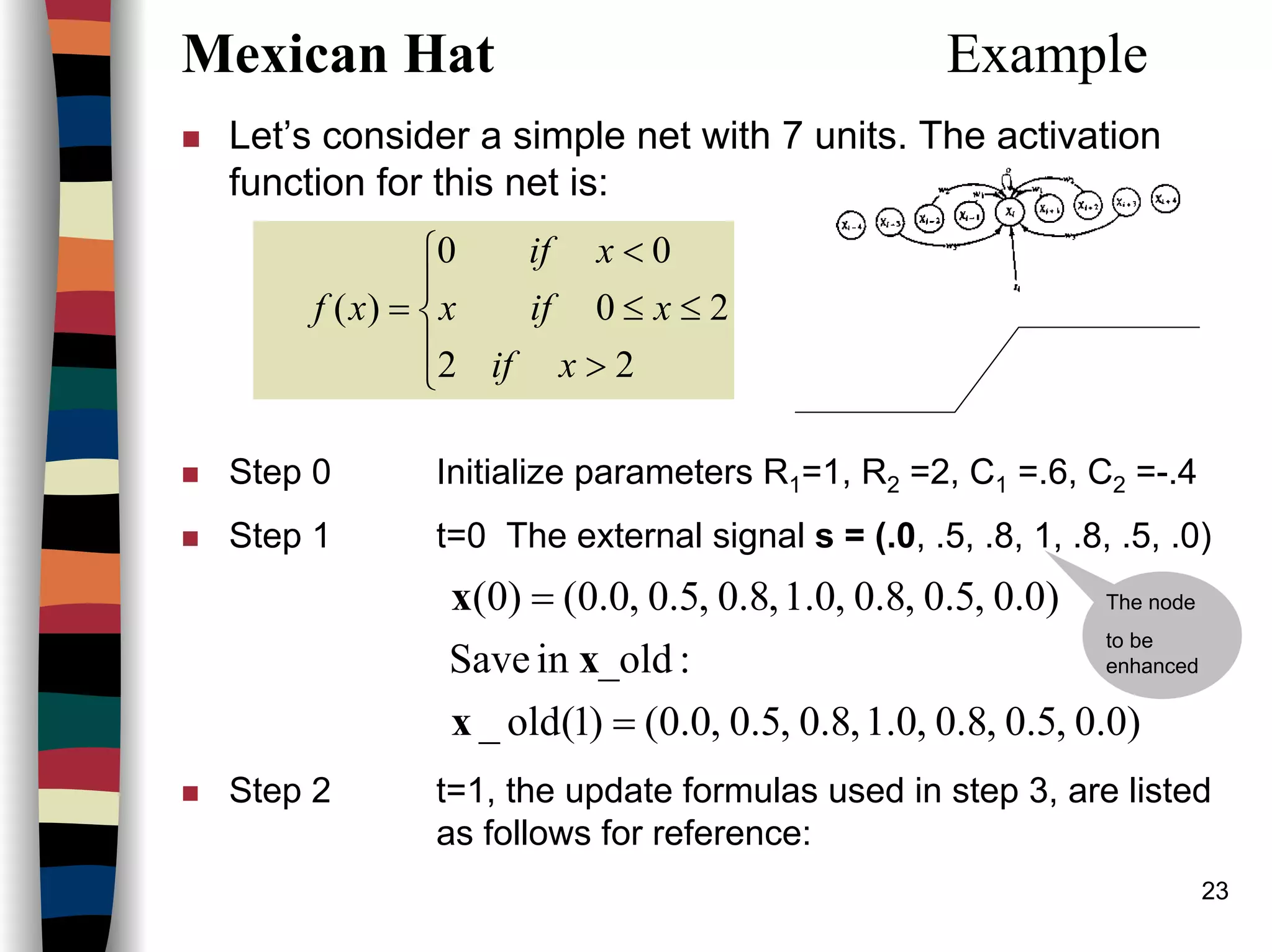
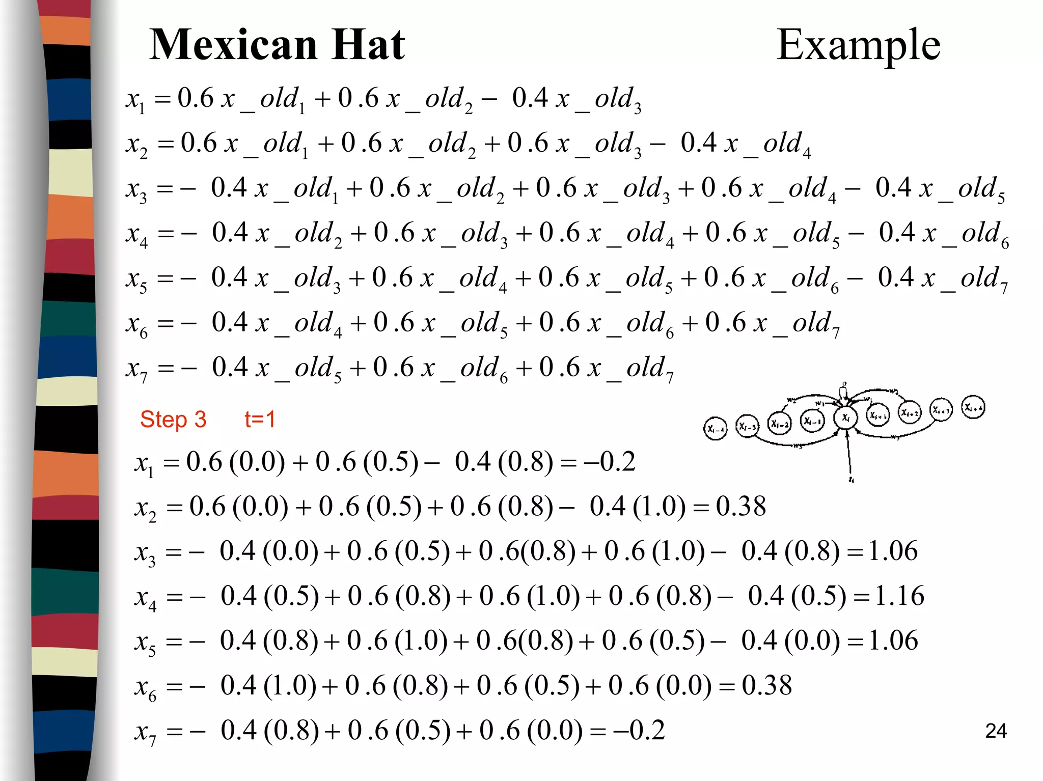
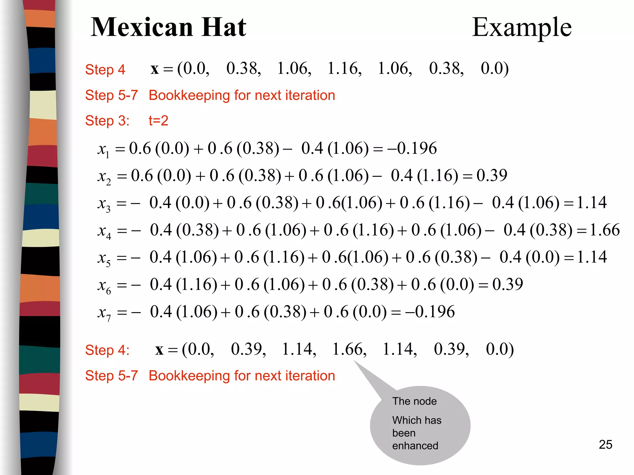
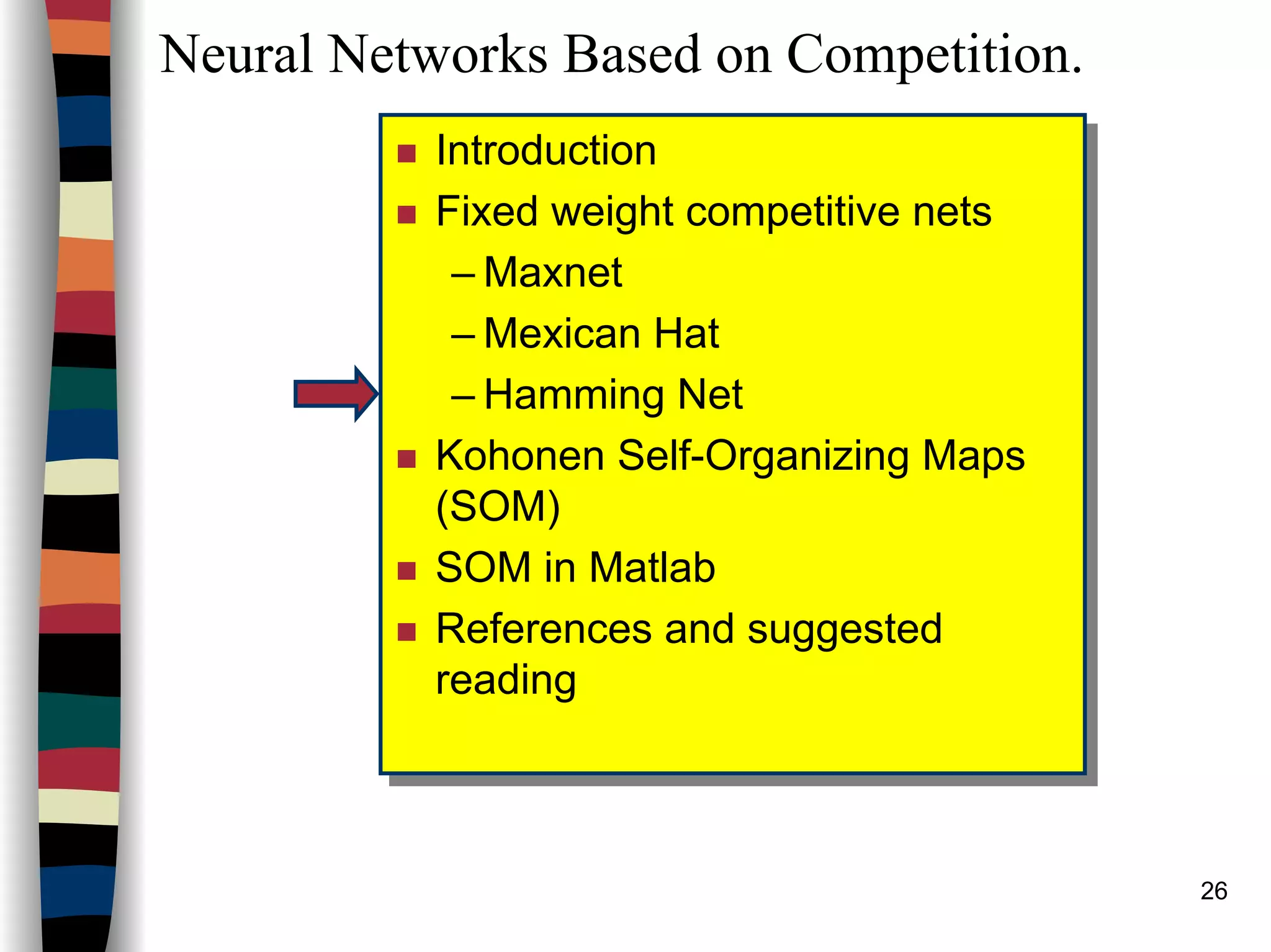
This document summarizes key concepts about neural networks based on competition. It discusses fixed weight competitive networks including Maxnet, Mexican Hat, and Hamming Net. Maxnet uses winner-take-all competition where only the neuron with the largest activation remains on. The Mexican Hat network enhances contrast through excitatory connections to nearby neurons and inhibitory connections to farther neurons. Iterating the activations over time steps increases the activation of neurons with initially larger signals and decreases others. Kohonen self-organizing maps and their training in Matlab are also mentioned.


![Competitive Learning [Deep Learning And Nueral Networks].pptx](https://cdn.slidesharecdn.com/ss_thumbnails/competitivelearning-240211053020-bc9a8437-thumbnail.jpg?width=640&height=640&fit=bounds)