The document discusses the challenges and methodologies for improving efficiency in Next Generation Sequencing (NGS) pipelines, particularly focusing on simple variant identification (SVI). It highlights the need for selective re-computation to minimize costs associated with processing updated genomic data while maintaining accuracy. The experiments demonstrate various approaches to optimize variant classification by assessing changes in input data and refining the re-execution process.

1. Simple Variant Identification
under ReComp control
Jacek Cała, Paolo Missier
Newcastle University
School of Computing Science

2. Outline
• Motivation – many computational problems, especially Big Data and
NGS pipelines, face an output deprecation issue
• updates of input data and tools make current results obsolete
• Test case – Simple Variant Identification
• pipeline-like structure, “small-data” process
• easy to implement and experiment with
• Experiments
• 3 different approaches compared with the baseline, blind re-computation
• provide insight into what selective re-computation can/cannot achieve
• Conclusions

3. The heavyweight of NGS pipelines
• NGS resequencing pipelines are an important example of the Big Data
analytics problems
• Important:
• Are at the core of the genomic analysis
• Big Data:
• raw sequences for WES analysis are measured in 1-20 GB per patient
• for quality purposes patient samples are usually processed in cohorts of 20-40
or close to 1 TB per cohort
• time required to process a 24-sample cohort can easily exceed 2 CPUmonths
• WES is only a fraction of what the WGS analyses require

4. Tracing change in the NGS resequencing
• Although the skeleton of the pipeline remains fairly static, many
aspects of the NGS are changing continuously
• Changes occur at various points and aspects of the pipeline but are
mainly two-fold:
• new tools and improved versions of the existing tools used at various steps in
the pipeline
• new updated reference and annotation data
• It is challenging to assess the impact of these changes on the output
of the pipeline
• the cost of rerunning the pipeline for all or even a cohort of patients is very
high

5. ReComp
• Aims to find ways to:
• detect and measure impact of changes in the input data
• allow the computational process to be selectively re-executed
• minimise the cost (runtime, monetary) of the re-execution with the maximum
benefit for the user
• One of the first steps – to run a part of the NGS pipeline under the
ReComp and evaluate potential benefits

6. The Simple Variant Identification tool
• Can help classify variants into three categories: RED, GREEN, AMBER
• pathogenic, benign and unknown
• uses OMIM GeneMap to identify genes- and variants-in-scope
• uses NCBI ClinVar to classify variants pathogenicity
• The SVI can be attached at the very end of an NGS pipeline
• as a simple, short running process can serve as a test scenario for ReComp
• SVI –> a mini-pipeline

7. High-level structure of the SVI process
Phenotype
to genes
genes in
scope
Variant
selection
<< input data >>
patient variants
(from a NGS pipeline)
<< input data >>
phenotype
hypothesis
<< reference data >>
OMIM GeneMap
<< reference data >>
NCBI ClinVar
<< output data >>
classified
variants
variants in
scope
Variant
classification
Simple Variant Identification

8. Detailed design of the SVI process
• Implemented as an e-Science Central workflow
• graphical design approach
• provenance tracking

9. Detailed design of the SVI process
Phenotype to genes
Variant selection
Variant classification
Patient
variants
GeneMap
ClinVar
Classified variants
Phenotype
hypothesis

10. Running SVI under ReComp
• A set of experiments designed to get insight into what and how
ReComp can help in process re-execution:
1. Blind re-computation
2. Partial re-computation
3. Partial re-computation using input difference
4. Partial re-computation with step-by-step impact analysis
• Experiments run on a set of 16 patients split by 4 different phenotype
hypotheses
• Tracking real changes in OMIM GeneMap and NCBI ClinVar

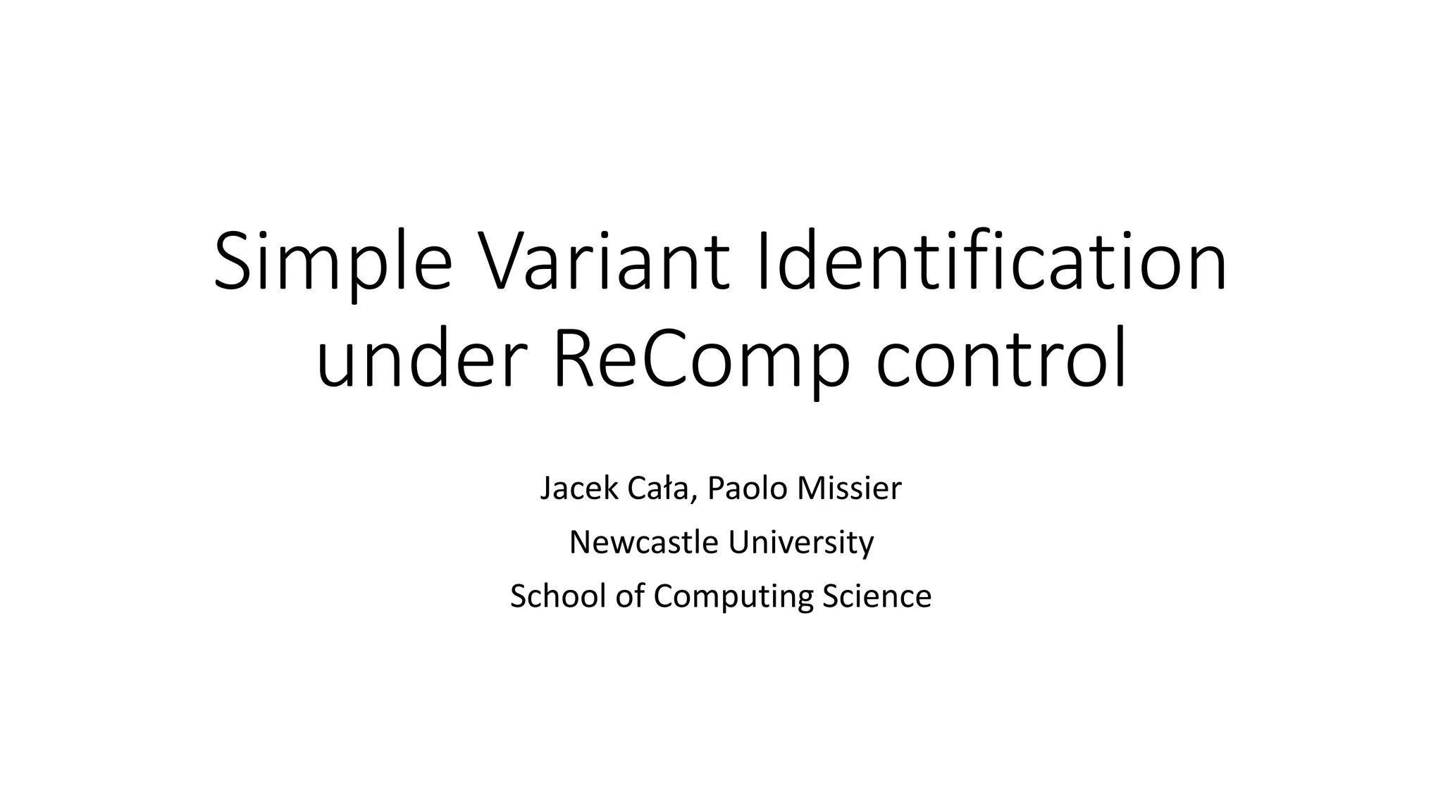
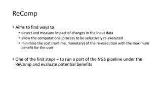
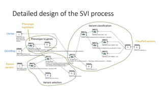
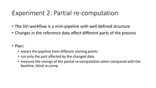
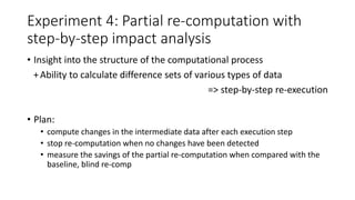
11. Experiments: Input data set
Phenotype hypothesis Variant file Variant count File size [MB]
Congenital myasthenic
syndrome
MUN0785 26508 35.5
MUN0789 26726 35.8
MUN0978 26921 35.8
MUN1000 27246 36.3
Parkinsons disease C0011 23940 38.8
C0059 24983 40.4
C0158 24376 39.4
C0176 24280 39.4
Creutzfeldt-Jakob disease A1340 23410 38.0
A1356 24801 40.2
A1362 24271 39.2
A1370 24051 38.9
Frontotemporal dementia -
Amyotrophic lateral sclerosis
B0307 24052 39.0
C0053 23980 38.8
C0171 24387 39.6
D1049 24473 39.5

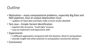
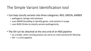
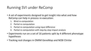
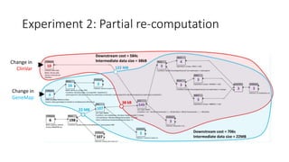
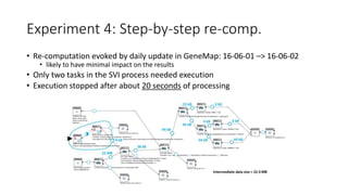
12. Experiments: Reference data sets
• Different rate of changes:
• GeneMap changes daily
• ClinVar changes monthly
Database Version
Record
count
File size
[MB]
OMIM
GeneMap
2016-03-08 13053 2.2
2016-04-28 15871 2.7
2016-06-01 15897 2.7
2016-06-02 15897 2.7
2016-06-07 15910 2.7
NCBI ClinVar 2015-02 281023 96.7
2016-02 285041 96.6
2016-05 290815 96.1

13. Experiment 1: Establishing the baseline –
blind re-computation
• Simple re-execution of the SVI process evoked by changes in
reference data (either GeneMap or ClinVar)
• Involves the maximum cost related to the execution of the process
• Blind re-computation is the baseline for the ReComp evaluation
• we want to be more effective than that

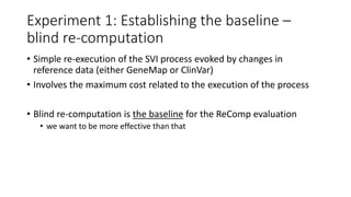
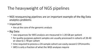
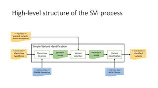
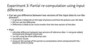
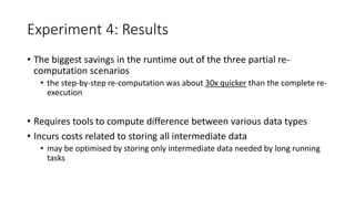
14. Experiment 1: Results
• Running the SVI workflow on one patient sample takes about 17
minutes
• executed on a single-core VM
• may be optimised –> optimisation out-of-scope at the moment
• Runtime is consistent across different phenotypes
• Changes of the GeneMap and ClinVar version have negligible impact
on the execution time, e.g.:
Run time [mm:ss]
GeneMap version 2016-03-08 2016-04-28 2016-06-07
μ ± σ 17:05 ± 22 17:09 ± 15 17:10 ± 17

15. Experiment 1: Results
• 17 min per sample => the SVI implementation has capacity of only 84
samples per CPUcore per day
• May be inadequate considering the daily rate of change of GeneMap
• Our goal is to increase this capacity through smart/selective re-
computation

16. Experiment 2: Partial re-computation
• The SVI workflow is a mini-pipeline with well defined structure
• Changes in the reference data affect different parts of the process
• Plan:
• restart the pipeline from different starting points
• run only the part affected by the changed data
• measure the savings of the partial re-computation when compared with the
baseline, blind re-comp

17. Experiment 2: Partial re-computation
Change in
ClinVar
Change in
GeneMap

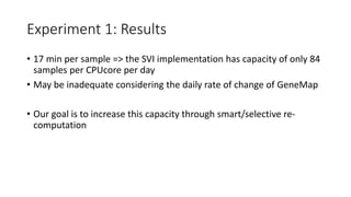
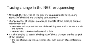
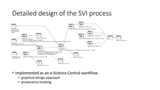
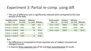
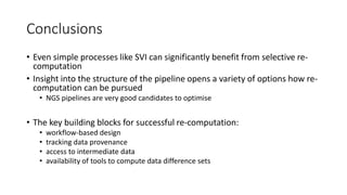
18. Experiment 2: Results
• Running the part of SVI directly involved in
processing updated data can save some
runtime
• Savings depend on:
• the structure of the process
• the point where the changed data are used
• Savings involve the cost of retaining interim
data required in partial re-execution
• the size of the data depends on the
phenotype hypothesis and type of change
• the size is in range of 20–22 MB for GeneMap
changes and 2–334 kB for ClinVar changes
Run time
[mm:ss]
Savings Run time
[mm:ss]
Savings
GeneMap
version
2016-04-28 2016-06-07
μ ± σ 11:51 ± 16 31% 11:50 ± 20 31%
ClinVar
version
2016-02 2016-05
μ ± σ 9:51 ± 14 43% 9:50 ± 15 42%

19. Experiment 3: Partial re-computation using input
difference
• Can we use difference between two versions of the input data to run the
process?
• In general, it depends on the type of process and how the process uses the data
• SVI can use the difference
• Difference is likely to be much smaller than the new version of the data
• Plan:
• calculate difference between two versions of reference data –> compute added,
removed and changed record sets
• run SVI using the three difference sets
• recombine results
• measure the savings of the partial re-computation when compared with the
baseline, blind re-comp

20. Experiment 3: Partial re-comp. using diff.
• The size of difference sets is significantly reduced when compared to the new
version of the data
but:
• the difference is computed as three separate sets of: added, removed and
changed records
• it requires three separate runs of SVI and then recombination of results
GeneMap versions
from –> to
ToVersion
rec. count
Difference
rec. count Reduction
16-03-08 –> 16-06-07 15910 1458 91%
16-03-08 –> 16-04-28 15871 1386 91%
16-04-28 –> 16-06-01 15897 78 99.5%
16-06-01 –> 16-06-02 15897 2 99.99%
16-06-02 –> 16-06-07 15910 33 99.8%
ClinVar versions
from –> to
ToVersion
rec. count
Difference
rec. count Reduction
15-02 –> 16-05 290815 38216 87%
15-02 –> 16-02 285042 35550 88%
16-02 –> 16-05 290815 3322 98.9%

21. Experiment 3: Results
• Running the part of SVI directly involved in
processing updated data can save some
runtime
• Running the part of SVI on each difference set
also saves some runtime
• Yet, the total cost of three separate re-
executions may exceed the savings
• Concluding, this approach has a few weak
points:
• running the process on diff. sets is not always
possible
• running the process using diff. sets requires
output recombination
• total runtime may sometimes exceed the
runtime of a regular update
Run time [mm:ss]
Added Removed Changed Total
GeneMap
change
11:30 ± 5 11:27 ± 11 11:36 ± 8 34:34 ± 16
ClinVar
change
2:29 ± 9 0:37 ± 7 0:44 ± 7 3:50 ± 22

22. Experiment 4: Partial re-computation with
step-by-step impact analysis
• Insight into the structure of the computational process
+Ability to calculate difference sets of various types of data
=> step-by-step re-execution
• Plan:
• compute changes in the intermediate data after each execution step
• stop re-computation when no changes have been detected
• measure the savings of the partial re-computation when compared with the
baseline, blind re-comp

23. Experiment 4: Step-by-step re-comp.
• Re-computation evoked by daily update in GeneMap: 16-06-01 –> 16-06-02
• likely to have minimal impact on the results
• Only two tasks in the SVI process needed execution
• Execution stopped after about 20 seconds of processing

24. Experiment 4: Results
• The biggest savings in the runtime out of the three partial re-
computation scenarios
• the step-by-step re-computation was about 30x quicker than the complete re-
execution
• Requires tools to compute difference between various data types
• Incurs costs related to storing all intermediate data
• may be optimised by storing only intermediate data needed by long running
tasks

25. Conclusions
• Even simple processes like SVI can significantly benefit from selective re-
computation
• Insight into the structure of the pipeline opens a variety of options how re-
computation can be pursued
• NGS pipelines are very good candidates to optimise
• The key building blocks for successful re-computation:
• workflow-based design
• tracking data provenance
• access to intermediate data
• availability of tools to compute data difference sets