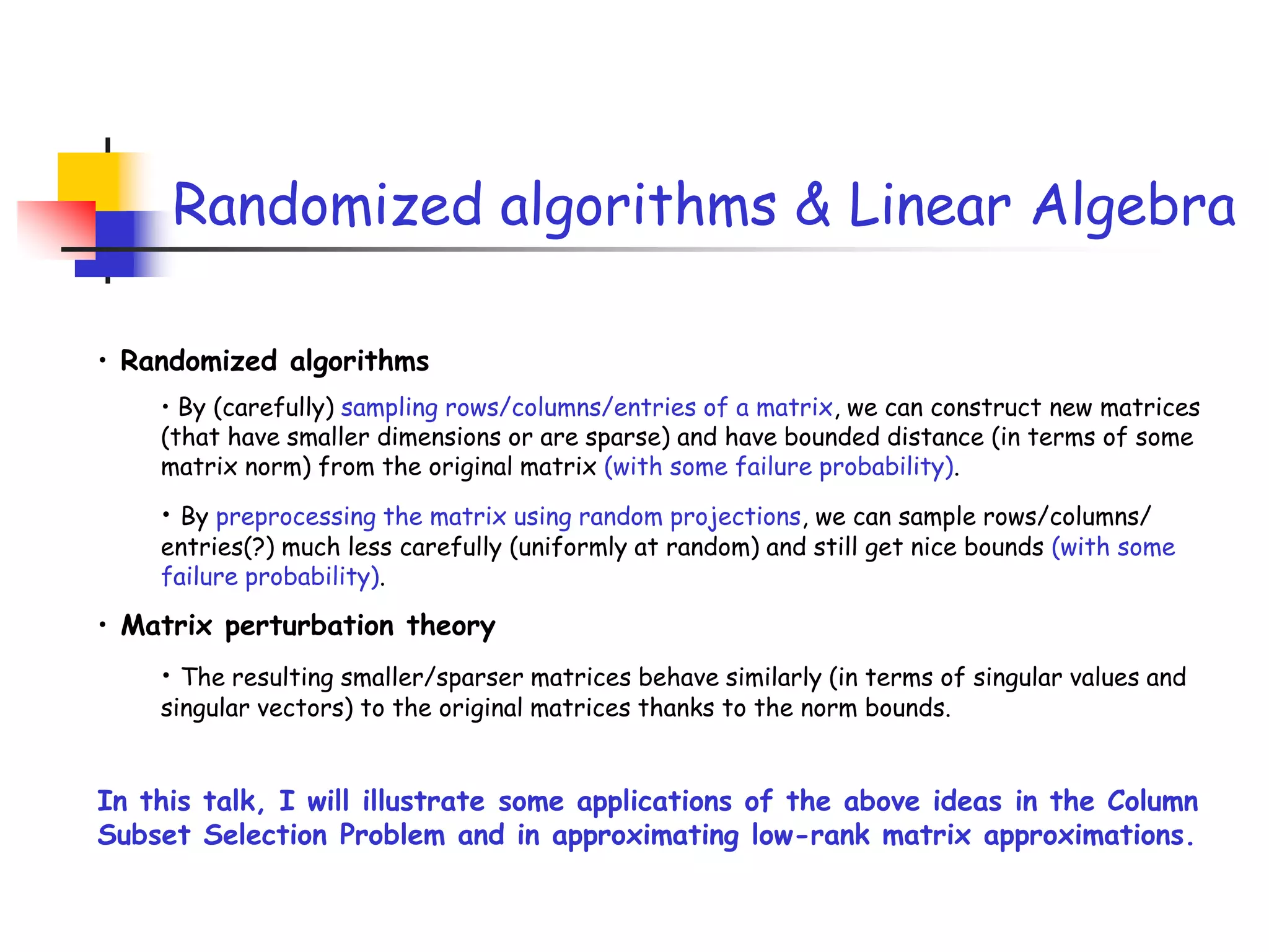
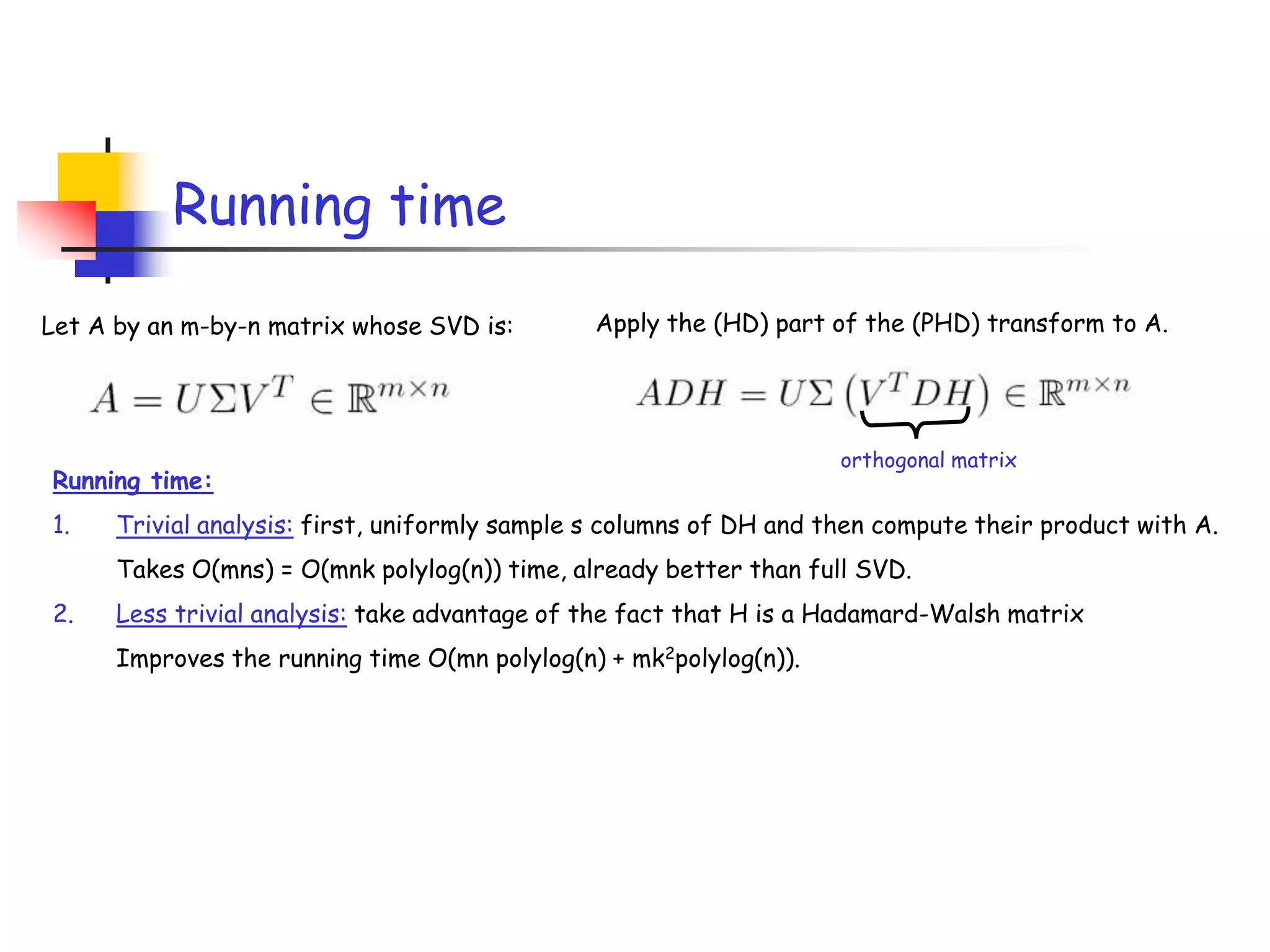
1) The document discusses randomized algorithms for linear algebra problems like matrix decomposition and column subset selection.
2) It describes how sampling rows/columns of a matrix using random projections can create smaller matrices that approximate the original well.
3) The talk will illustrate applications of these ideas to the column subset selection problem and approximating low-rank matrix decompositions.
Scalabiltity in GBML, Accuracy-based Michigan Fuzzy LCS, and new TrendsXavier Llorà
The document summarizes a presentation given by Jorge Casillas on research related to scaling up genetic learning algorithms and fuzzy classifier systems. Specifically, it discusses:
1. An approach using evolutionary instance selection and stratification to extract rule sets from large datasets that balance prediction accuracy and interpretability.
2. Fuzzy-XCS, an accuracy-based genetic fuzzy system the author is developing that uses competitive fuzzy inference and represents rules as disjunctive normal forms to address challenges in credit assignment.
3. Open problems and opportunities in applying genetic learning at large scales, such as addressing chromosome size and efficient evaluation over large datasets.
The document describes several algorithms for dynamic programming and graph algorithms:
1. It presents four algorithms for computing the Fibonacci numbers using dynamic programming with arrays or recursion with and without memoization.
2. It provides algorithms for solving coin changing and matrix multiplication problems using dynamic programming by filling out arrays.
3. It gives algorithms to find the length and a longest common subsequence between two strings using dynamic programming.
4. It introduces algorithms to find shortest paths between all pairs of vertices in a weighted graph using Floyd's and Warshall's algorithms. It includes algorithms to output a shortest path between two vertices.
Dynamic programming in Algorithm AnalysisRajendran
The document discusses dynamic programming and amortized analysis. It covers:
1) An example of amortized analysis of dynamic tables, where the worst case cost of an insert is O(n) but the amortized cost is O(1).
2) Dynamic programming can be used when a problem breaks into recurring subproblems. Longest common subsequence is given as an example that is solved using dynamic programming in O(mn) time rather than a brute force O(2^m*n) approach.
3) The dynamic programming algorithm for longest common subsequence works by defining a 2D array c where c[i,j] represents the length of the LCS of the first i elements
This document discusses Warshall's algorithm for finding the transitive closure of a graph using dynamic programming. It begins with an introduction to transitive closure and how it relates to Facebook vs Google+ graph types. It then provides an explanation of Warshall's algorithm, including a visitation example and weighted example. It analyzes the time and space complexity of Warshall's algorithm as O(n3) and O(n2) respectively. It concludes with applications of Warshall's algorithm such as shortest paths and bipartite graph checking.
Dynamic Programming is a method for solving a complex problem by breaking it down into a collection of simpler subproblems, solving each of those subproblems just once, and storing their solutions using a memory-based data structure (array, map,etc).
This document discusses algorithms and dynamic programming techniques. It focuses on iterative algorithms for calculating Fibonacci numbers and edit distance, including applications in computational molecular biology such as finding the longest common subsequence and comparing sequences with mismatches. Edit distance is explored in depth through iterative formulations and applications.
The Shortest Path Tour Problem is an extension to the normal Shortest Path Problem and appeared in the scientific literature in Bertsekas's dynamic programming and optimal control book in 2005, for the first time. This paper gives a description of the problem, two algorithms to solve it. Results to the numeric experimentation are given in terms of graphs. Finally, conclusion and discussions are made.
The document discusses the problem solving technique of backtracking. Backtracking involves making a series of decisions with limited information, where each decision leads to further choices. It explores potential solutions systematically by trying choices and abandoning ("backtracking") from choices that do not lead to solutions. Examples where backtracking can be applied include solving mazes, map coloring problems, and puzzles. The key aspects of backtracking are exploring potential solutions through recursion or looping, checking if a partial solution can be completed at each choice, and abandoning incomplete solutions that cannot be completed.
Dynamic programming is an algorithmic technique that solves problems by breaking them down into smaller subproblems and storing the results of subproblems to avoid recomputing them. It is useful for optimization problems with overlapping subproblems. The key steps are to characterize the structure of an optimal solution, recursively define the value of an optimal solution, compute that value, and construct the optimal solution. Examples discussed include rod cutting, longest increasing subsequence, longest palindrome subsequence, and palindrome partitioning. Other problems that can be solved with dynamic programming include edit distance, shortest paths, optimal binary search trees, the traveling salesman problem, and reliability design.
The document discusses various backtracking algorithms and problems. It begins with an overview of backtracking as a general algorithm design technique for problems that involve traversing decision trees and exploring partial solutions. It then provides examples of specific problems that can be solved using backtracking, including the N-Queens problem, map coloring problem, and Hamiltonian circuits problem. It also discusses common terminology and concepts in backtracking algorithms like state space trees, pruning nonpromising nodes, and backtracking when partial solutions are determined to not lead to complete solutions.
Subset sum problem Dynamic and Brute Force ApprochIjlal Ijlal
The document discusses the subset sum problem and approaches to solve it. It begins by defining the problem and providing an example. It then analyzes the brute force approach of checking all possible subsets and calculates its exponential time complexity. The document introduces dynamic programming as an efficient alternative, providing pseudocode for a dynamic programming algorithm that solves the problem in polynomial time by storing previously computed solutions. It concludes by discussing applications of similar problems in traveling salesperson and drug discovery.
What is the Covering (Rule-based) algorithm?
Classification Rules- Straightforward
1. If-Then rule
2. Generating rules from Decision Tree
Rule-based Algorithm
1. The 1R Algorithm / Learn One Rule
2. The PRISM Algorithm
3. Other Algorithm
Application of Covering algorithm
Discussion on e/m-learning application
Backtracking is a general algorithm for finding all (or some) solutions to some computational problems, notably constraint satisfaction problems, that incrementally builds candidates to the solutions, and abandons each partial candidate c ("backtracks") as soon as it determines that c cannot possibly be completed to a valid solution.
Constraint satisfaction problems (CSPs) define states as assignments of variables to values from their domains, with constraints specifying allowable combinations. Backtracking search assigns one variable at a time using depth-first search. Improved heuristics like most-constrained variable selection and least-constraining value choice help. Forward checking and constraint propagation techniques like arc consistency detect inconsistencies earlier than backtracking alone. Local search methods like min-conflicts hill-climbing can also solve CSPs by allowing constraint violations and minimizing them.
Backtracking is used to systematically search for solutions to problems by trying possibilities and abandoning ("backtracking") partial candidate solutions that fail to satisfy constraints. Examples discussed include the rat in a maze problem, the traveling salesperson problem, container loading, finding the maximum clique in a graph, and board permutation problems. Backtracking algorithms traverse the search space depth-first and use pruning techniques like discarding partial solutions that cannot lead to better complete solutions than those already found.
This document discusses data structures and algorithms related to queues. It defines queues as first-in first-out (FIFO) linear lists and describes common queue operations like offer(), poll(), peek(), and isEmpty(). Implementations of queues using linked lists and circular arrays are presented. Applications of queues include accessing shared resources and serving as components of other data structures. The document concludes by explaining the eight queens puzzle and presenting an algorithm to solve it using backtracking.
The document discusses various backtracking techniques including bounding functions, promising functions, and pruning to avoid exploring unnecessary paths. It provides examples of problems that can be solved using backtracking including n-queens, graph coloring, Hamiltonian circuits, sum-of-subsets, 0-1 knapsack. Search techniques for backtracking problems include depth-first search (DFS), breadth-first search (BFS), and best-first search combined with branch-and-bound pruning.
Backtracking and branch and bound are algorithms used to solve problems with large search spaces. Backtracking uses depth-first search and prunes subtrees that don't lead to viable solutions. Branch and bound uses breadth-first search and pruning, maintaining partial solutions in a priority queue. Both techniques systematically eliminate possibilities to find optimal solutions faster than exhaustive search. Examples where they can be applied include maze pathfinding, the eight queens problem, sudoku, and the traveling salesman problem.
Backtracking is a general algorithm for finding all (or some) solutions to some computational problems, notably constraint satisfaction problems, that incrementally builds candidates to the solutions, and abandons each partial candidate c ("backtracks") as soon as it determines that c cannot possibly be completed to a valid solution.
Analysis of Feature Selection Algorithms (Branch & Bound and Beam search)Parinda Rajapaksha
Branch & Bound and Beam search algorithms were illustrated according to the feature selection domain. Presentation is structured as follows,
- Motivation
- Introduction
- Analysis
- Algorithm
- Pseudo Code
- Illustration of examples
- Applications
- Observations and Recommendations
- Comparison between two algorithms
- References
The document discusses backtracking, which is a technique for solving constraint satisfaction problems using three basic colors (R, G, B) to color graphs without conflicts. It provides rules for using only three colors with no conflicts and describes the backtracking approach. It then provides four practice graph coloring problems to solve using backtracking.
The document describes the backtracking method for solving problems that require finding optimal solutions. Backtracking involves building a solution one component at a time and using bounding functions to prune partial solutions that cannot lead to an optimal solution. It then provides examples of applying backtracking to solve the 8 queens problem by placing queens on a chessboard with no attacks. The general backtracking method and a recursive backtracking algorithm are also outlined.
The document discusses solving the 8 queens problem using backtracking. It begins by explaining backtracking as an algorithm that builds partial candidates for solutions incrementally and abandons any partial candidate that cannot be completed to a valid solution. It then provides more details on the 8 queens problem itself - the goal is to place 8 queens on a chessboard so that no two queens attack each other. Backtracking is well-suited for solving this problem by attempting to place queens one by one and backtracking when an invalid placement is found.
The document discusses the knapsack problem, which involves selecting a subset of items that fit within a knapsack of limited capacity to maximize the total value. There are two versions - the 0-1 knapsack problem where items can only be selected entirely or not at all, and the fractional knapsack problem where items can be partially selected. Solutions include brute force, greedy algorithms, and dynamic programming. Dynamic programming builds up the optimal solution by considering all sub-problems.
The document provides an overview of graph concepts including definitions of a graph as a pair of vertices and edges, different types of graphs such as directed/undirected graphs and cyclic/acyclic graphs. It also discusses graph coloring, adjacency matrices/lists for representing graphs, and algorithms for traversing graphs including depth-first search and breadth-first search. Examples are given for each concept to illustrate key differences and properties.
Structured Query Language (SQL) - Lecture 5 - Introduction to Databases (1007...Beat Signer
The document discusses Structured Query Language (SQL) and its history and components. It notes that SQL is a declarative query language used to define database schemas, manipulate data through queries, and control transactions. The document outlines SQL's data definition language for defining schemas and data manipulation language for querying and modifying data. It also provides examples of SQL statements for creating tables and defining constraints.
Matrix Factorizations at Scale: a Comparison of Scientific Data Analytics on ...Databricks
This document discusses computationally intensive machine learning at large scales. It compares the algorithmic and statistical perspectives of computer scientists and statisticians when analyzing big data. It describes three science applications that use linear algebra techniques like PCA, NMF and CX decompositions on large datasets. Experiments are presented comparing the performance of these techniques implemented in Spark and MPI on different HPC platforms. The results show Spark can be 4-26x slower than optimized MPI codes. Next steps proposed include developing Alchemist to interface Spark and MPI more efficiently and exploring communication-avoiding machine learning algorithms.
The document describes the sequencing of the wheat genome, specifically chromosome 3B. Key points:
1. An international effort led by the IWGSC sequenced individual wheat chromosomes including 3B using a physical map-based approach.
2. Sequencing of the 1Gb chromosome 3B generated over 1000 scaffolds covering 995Mb with an N50 of 463kb. Genes and markers were annotated.
3. The sequenced and ordered chromosome 3B provides a foundation for accelerating wheat improvement through map-based cloning, marker development, and integrating genetic and genomic resources.
This document reanalyzes ancient mitochondrial DNA sequences recovered from Neandertal bones. Previous studies placed Neandertals at the base of the modern human phylogenetic tree, suggesting they did not contribute to the modern human gene pool. However, these analyses did not account for high substitution rate variation among sites in the human mitochondrial D-loop region or estimate nucleotide substitution model parameters. The authors reanalyze the Neandertal sequences using maximum likelihood methods that account for these factors to provide a more accurate phylogenetic reconstruction.
The document summarizes the Genome in a Bottle Consortium's unprecedented characterization of human reference genomes, including two trios. It describes how the consortium has generated extensive genomic data from various technologies for these genomes and is developing high-confidence calls for variants including SNPs, indels, and structural variants. The consortium is working to characterize more difficult variants and regions, and welcomes new collaborations to further characterize the genomes.
This document summarizes genetic variation projects like HapMap and 1000 Genomes that aimed to catalog common human genetic variants. It describes types of variation like SNPs and how factors like selection and recombination influence their distribution. It provides overviews of the HapMap and 1000 Genomes projects, including their goals, populations studied, methods, and data formats. The information from these projects can be used to study traits, diseases, and human history.
1. Icarus is a DNA walking program that plots DNA sequences in 2D space by assigning directions to nucleotide bases and having a virtual walker take steps in those directions as the sequence is read off.
2. DNA walks can reveal structural elements and repetitive regions in sequences as repetitive patterns.
3. Icarus was demonstrated to identify a duplication in a Y chromosome by accident through a DNA walk, whereas traditional methods required complex scripts.
4. While spatial distances from DNA walks can produce phylogenies, a better distance measure is needed than simple Euclidean or Manhattan distance as walks can be influenced by nucleotide composition and sequence order.
This document summarizes an academic presentation about algorithms for aligning genomic sequences. It discusses edit distance models for comparing sequences and finding the best alignment. Local, global, and glocal alignment algorithms are introduced, including CHAOS for local alignment and LAGAN and Shuffle-LAGAN for multiple global and glocal alignments of whole genomes. Applications to aligning the cystic fibrosis gene and analyzing rearrangements between human and mouse are also summarized.
Karen miga centromere sequence characterization and variant detectionGenomeInABottle
Centromeric regions contain significant human genetic variation that is not represented in current reference genomes. This document proposes a two-part approach to characterize sequence variation in centromeric regions: (1) construct chromosome-specific reference maps of centromeric DNA, and (2) expand the human variation reference map to include centromeric regions. Key aspects include using long reads to assemble higher-order repeats, short reads to estimate array sizes and variant frequencies, and graph representations to model structural variation while retaining haplotype information. This would provide new insights into centromeric biology and identify centromeric variants associated with disease.
Global Modeling of Biodiversity and Climate ChangeSalford Systems
This document provides an overview of global modeling of biodiversity and climate change conducted by the EWHALE lab at the University of Alaska Fairbanks. It discusses the lab's use of spatial/geographic information systems and machine learning to make predictions about species distributions and impacts of factors like climate change. The lab utilizes various machine learning algorithms like random forests and boosted regression trees to build predictive models using environmental data and species occurrence records. Students and projects at the lab apply these modeling approaches to questions about Arctic seabirds and other species globally.
The document discusses next generation sequencing methods and RNA sequencing. It covers topics like sequencing formats, data analysis workflows including mapping, clustering, assembly programs, finding new genes and correcting existing ones. It discusses input file types, calculating sequencing depth, available tools for alignment, output file formats, assembly programs, splice junction prediction, and applications of RNA sequencing like gene expression analysis and annotation.
The document discusses the Genome in a Bottle Consortium's efforts to develop whole genome reference samples and characterize genetic variants, including small variants and structural variants. It provides details on 5 reference genomes that have been extensively characterized and released as reference materials. The challenges of characterizing more difficult variants like large indels and structural variants are also discussed.
This document summarizes the Wheat Genome Project. It discusses:
1) The goals of the project which are to lay a foundation to accelerate wheat improvement and increase profitability throughout the industry.
2) The current status of the project which has sequenced and assembled 40 chromosome arms totaling 10.2 Gb and annotated over 124,000 genes.
3) Future applications of the project resources which will include high density SNP chips, analyses of wheat genome evolution and gene expression, and facilitating map-based cloning of important wheat genes.
RNA-seq: A High-resolution View of the TranscriptomeSean Davis
The molecular microscopes that we use to examine human biology have advanced significantly with the advent of next generation sequencing. RNA-seq is one application of this technology that leads to a very high-resolution view of the transcriptome. With these new technologies come increased data analysis and data handling burdens as well as the promise of new discovery. These slides present a high-level overview of the RNA-seq technology with a focus on the analysis approaches, quality control challenges, and experimental design.
Next generation sequencing techniques were discussed including an overview of various sequencing platforms, their output, and common analysis workflows. Mapping short reads to reference genomes using alignment programs is a key first step for most applications. Formats like FASTQ, SAM, and BAM are commonly used to store sequencing reads and mapping results.
Human genetic variation and its contribution to complex traitsgroovescience
This document summarizes a meeting discussing the human genome and human genetic variation.
The key points are:
1) In June 2000, the first draft of the human genome was announced, with fully sequenced publications in 2001. This marked a major milestone in understanding the human genome.
2) Since then, over 11 million SNPs and thousands of structural variants have been discovered through projects like HapMap and large sequencing studies. However, the majority of rare variants are still unknown.
3) Genome-wide association studies since 2006 have identified over 300 genetic loci associated with over 80 human traits and diseases. However, determining the functional consequences and molecular mechanisms remains a major challenge.
Humans continue to evolve through the processes of mutation, natural selection, genetic drift, and gene flow. While the human brain has shrunk in size over thousands of years, culture accelerates human evolution. Selection pressures like malaria, sickle cell anemia, and infectious diseases drive ongoing genetic changes in populations. With a global population of billions, unprecedented human genetic diversity and millions of new mutations arising every generation, human evolution is active and ongoing.
Presentation by Benedict Paten at GRC/GIAB ASHG 2017 workshop "Getting the most from the reference assembly and reference materials" on updates to the human reference assembly, GRCh38.
In this deck from the Perth HPC Conference, Rob Farber from TechEnablement presents: AI is Impacting HPC Everywhere.
"The convergence of AI and HPC has created a fertile venue that is ripe for imaginative researchers — versed in AI technology — to make a big impact in a variety of scientific fields. From new hardware to new computational approaches, the true impact of deep- and machine learning on HPC is, in a word, “everywhere”. Just as technology changes in the personal computer market brought about a revolution in the design and implementation of the systems and algorithms used in high performance computing (HPC), so are recent technology changes in machine learning bringing about an AI revolution in the HPC community. Expect new HPC analytic techniques including the use of GANs (Generative Adversarial Networks) in physics-based modeling and simulation, as well as reduced precision math libraries such as NLAFET and HiCMA to revolutionize many fields of research. Other benefits of the convergence of AI and HPC include the physical instantiation of data flow architectures in FPGAs and ASICs, plus the development of powerful data analytic services."
Learn more: http://www.techenablement.com/
and
http://hpcadvisorycouncil.com/events/2019/australia-conference/agenda.php
Sign up for our insideHPC Newsletter: http://insidehpc.com/newsletter
Similar to Randomized Algorithms in Linear Algebra & the Column Subset Selection Problem (20)
Randomized Algorithms in Linear Algebra & the Column Subset Selection Problem
1. Randomized Algorithms in Linear Algebra
& the Column Subset Selection Problem
Petros Drineas
Rensselaer Polytechnic Institute
Computer Science Department
To access my web page:
drineas
2. Randomized algorithms & Linear Algebra
• Randomized algorithms
• By (carefully) sampling rows/columns/entries of a matrix, we can construct new matrices
(that have smaller dimensions or are sparse) and have bounded distance (in terms of some
matrix norm) from the original matrix (with some failure probability).
• By preprocessing the matrix using random projections (*), we can sample rows/columns/
entries(?) much less carefully (uniformly at random) and still get nice bounds (with some
failure probability).
(*) Alternatively, we can assume that the matrix is “well-behaved” and thus uniform sampling will work.
3. Randomized algorithms & Linear Algebra
• Randomized algorithms
• By (carefully) sampling rows/columns/entries of a matrix, we can construct new matrices
(that have smaller dimensions or are sparse) and have bounded distance (in terms of some
matrix norm) from the original matrix (with some failure probability).
• By preprocessing the matrix using random projections, we can sample rows/columns/
entries(?) much less carefully (uniformly at random) and still get nice bounds (with some
failure probability).
• Matrix perturbation theory
• The resulting smaller/sparser matrices behave similarly (in terms of singular values and
singular vectors) to the original matrices thanks to the norm bounds.
In this talk, I will illustrate some applications of the above ideas in the Column
Subset Selection Problem and in approximating low-rank matrix approximations.
4. Interplay
(Data Mining) Applications
Biology & Medicine: population genetics (coming up…)
Electrical Engineering: testing of electronic circuits
Internet Data: recommendation systems, document-term data
Theoretical Computer Science Numerical Linear Algebra
Randomized and approximation Matrix computations and Linear
algorithms Algebra (ie., perturbation theory)
5. Human genetics
Single Nucleotide Polymorphisms: the most common type of genetic variation in the
genome across different individuals.
They are known locations at the human genome where two alternate nucleotide bases
(alleles) are observed (out of A, C, G, T).
SNPs
… AG CT GT GG CT CC CC CC CC AG AG AG AG AG AA CT AA GG GG CC GG AG CG AC CC AA CC AA GG TT AG CT CG CG CG AT CT CT AG CT AG GG GT GA AG …
individuals
… GG TT TT GG TT CC CC CC CC GG AA AG AG AG AA CT AA GG GG CC GG AA GG AA CC AA CC AA GG TT AA TT GG GG GG TT TT CC GG TT GG GG TT GG AA …
… GG TT TT GG TT CC CC CC CC GG AA AG AG AA AG CT AA GG GG CC AG AG CG AC CC AA CC AA GG TT AG CT CG CG CG AT CT CT AG CT AG GG GT GA AG …
… GG TT TT GG TT CC CC CC CC GG AA AG AG AG AA CC GG AA CC CC AG GG CC AC CC AA CG AA GG TT AG CT CG CG CG AT CT CT AG CT AG GT GT GA AG …
… GG TT TT GG TT CC CC CC CC GG AA GG GG GG AA CT AA GG GG CT GG AA CC AC CG AA CC AA GG TT GG CC CG CG CG AT CT CT AG CT AG GG TT GG AA …
… GG TT TT GG TT CC CC CG CC AG AG AG AG AG AA CT AA GG GG CT GG AG CC CC CG AA CC AA GT TT AG CT CG CG CG AT CT CT AG CT AG GG TT GG AA …
… GG TT TT GG TT CC CC CC CC GG AA AG AG AG AA TT AA GG GG CC AG AG CG AA CC AA CG AA GG TT AA TT GG GG GG TT TT CC GG TT GG GT TT GG AA …
Matrices including thousands of individuals and hundreds of thousands if SNPs are available.
6. HGDP data
• 1,033 samples
• 7 geographic regions
• 52 populations
The Human Genome Diversity Panel (HGDP)
Cavalli-Sforza (2005) Nat Genet Rev
Rosenberg et al. (2002) Science
Li et al. (2008) Science
7. CEU HGDP data
• 1,033 samples
• 7 geographic regions
• 52 populations
TSI
JPT, CHB, & CHD
HapMap Phase 3 data
MEX • 1,207 samples
GIH • 11 populations
ASW, MKK,
LWK, & YRI
HapMap Phase 3
The Human Genome Diversity Panel (HGDP)
Cavalli-Sforza (2005) Nat Genet Rev
Rosenberg et al. (2002) Science
Li et al. (2008) Science
The International HapMap Consortium
(2003, 2005, 2007) Nature
8. CEU HGDP data
• 1,033 samples
• 7 geographic regions
• 52 populations
TSI
JPT, CHB, & CHD
HapMap Phase 3 data
MEX • 1,207 samples
GIH • 11 populations
ASW, MKK,
LWK, & YRI
HapMap Phase 3 We will apply SVD/PCA
on the (joint) HGDP and
The Human Genome Diversity Panel (HGDP) HapMap Phase 3 data.
Matrix dimensions:
2,240 subjects (rows)
447,143 SNPs (columns)
Dense matrix:
Cavalli-Sforza (2005) Nat Genet Rev over one billion entries
Rosenberg et al. (2002) Science
Li et al. (2008) Science
The International HapMap Consortium
(2003, 2005, 2007) Nature
9. The Singular Value Decomposition (SVD)
5 Let the blue circles represent m
data points in a 2-D Euclidean space.
Then, the SVD of the m-by-2 matrix
of the data will return …
4
3
2
4.0 4.5 5.0 5.5 6.0
10. The Singular Value Decomposition (SVD)
5 Let the blue circles represent m
data points in a 2-D Euclidean space.
Then, the SVD of the m-by-2 matrix
of the data will return …
4
1st (right) singular vector:
direction of maximal variance,
3
1st (right)
singular vector
2
4.0 4.5 5.0 5.5 6.0
11. The Singular Value Decomposition (SVD)
5 Let the blue circles represent m
data points in a 2-D Euclidean space.
2nd (right)
singular vector Then, the SVD of the m-by-2 matrix
of the data will return …
4
1st (right) singular vector:
direction of maximal variance,
3
2nd (right) singular vector:
1st (right)
singular vector
direction of maximal variance, after
removing the projection of the data
2 along the first singular vector.
4.0 4.5 5.0 5.5 6.0
12. Singular values
5
1: measures how much of the data variance
is explained by the first singular vector.
2nd (right) 2
singular vector
2: measures how much of the data variance
is explained by the second singular vector.
4
Principal Components Analysis (PCA) is done via the
computation of the Singular Value Decomposition
3 (SVD) of a (mean-centered) covariance matrix.
1
1st (right)
singular vector Typically, a small constant number (say k) of the
top singular vectors and values are kept.
2
4.0 4.5 5.0 5.5 6.0
13. CEU HGDP data
• 1,033 samples
• 7 geographic regions
• 52 populations
TSI
JPT, CHB, & CHD
HapMap Phase 3 data
MEX • 1,207 samples
GIH • 11 populations
ASW, MKK,
LWK, & YRI
Matrix dimensions:
2,240 subjects (rows)
HapMap Phase 3
447,143 SNPs (columns)
The Human Genome Diversity Panel (HGDP)
SVD/PCA
returns…
Cavalli-Sforza (2005) Nat Genet Rev
Rosenberg et al. (2002) Science
Li et al. (2008) Science
The International HapMap Consortium
(2003, 2005, 2007), Nature
14. Paschou, Lewis, Javed, & Drineas (2010) J Med Genet
Europe
Middle East
Gujarati
Indians
South Central
Mexicans Asia
Africa
Oceania
America
East Asia
• Top two Principal Components (PCs or eigenSNPs)
(Lin and Altman (2005) Am J Hum Genet)
• The figure renders visual support to the “out-of-Africa” hypothesis.
• Mexican population seems out of place: we move to the top three PCs.
15. Paschou, Lewis, Javed, & Drineas (2010) J Med Genet
Africa
Middle East
S C Asia &
Gujarati Europe
Oceania
East Asia
America
Not altogether satisfactory: the principal components are linear combinations
of all SNPs, and – of course – can not be assayed!
Can we find actual SNPs that capture the information in the singular vectors?
Formally: spanning the same subspace.
16. Issues
• Computing large SVDs: computational time
• In commodity hardware (e.g., a 4GB RAM, dual-core laptop), using MatLab 7.0 (R14), the
computation of the SVD of the dense 2,240-by-447,143 matrix A takes about 12 minutes.
• Computing this SVD is not a one-liner, since we can not load the whole matrix in RAM
(runs out-of-memory in MatLab).
• We compute the eigendecomposition of AAT.
• In a similar experiment, we computed 1,200 SVDs on matrices of dimensions (approx.)
1,200-by-450,000 (roughly speaking a full leave-one-out cross-validation experiment).
(Drineas, Lewis, & Paschou (2010) PLoS ONE)
• Obviously, running time is a concern.
• We need efficient, easy to implement, methods.
17. Issues (cont’d)
• Selecting good columns that “capture the structure” of the top PCs
• Combinatorial optimization problem; hard even for small matrices.
• Often called the Column Subset Selection Problem (CSSP).
• Not clear that such columns even exist.
18. Issues (cont’d)
• Selecting good columns that “capture the structure” of the top PCs
• Combinatorial optimization problem; hard even for small matrices.
• Often called the Column Subset Selection Problem (CSSP).
• Not clear that such columns even exist.
Such datasets will only continue to increase in size:
In collaboration with K. Kidd’s lab (Yale University, Department of Genetics) we are
now analyzing:
• 4,000 samples from over 100 populations
• genotyped on over 500,000 SNPs.
19. Our perspective
The two issues are connected
• There exist “good” columns in any matrix that contain information about the
top principal components.
• We can identify such columns via a simple statistic: the leverage scores.
• This does not immediately imply faster algorithms for the SVD, but, combined
with random projections, it does!
20. SVD decomposes a matrix as…
The SVD has strong
optimality properties.
Top k left singular vectors
It is easy to see that X = UkTA.
SVD has strong optimality properties.
The columns of Uk are linear combinations of up to all columns of A.
21. The CX decomposition
Drineas, Mahoney, & Muthukrishnan (2008) SIAM J Mat Anal Appl
Mahoney & Drineas (2009) PNAS
Carefully
chosen X
Goal: make (some norm) of A-CX small.
c columns of A
Why?
If A is an subject-SNP matrix, then selecting representative columns is
equivalent to selecting representative SNPs to capture the same structure
as the top eigenSNPs.
We want c as small as possible!
22. CX decomposition
c columns of A
Easy to prove that optimal X = C+A. (C+ is the Moore-Penrose pseudoinverse of C.)
Thus, the challenging part is to find good columns (SNPs) of A to include in C.
From a mathematical perspective, this is a hard combinatorial problem, closely
related to the so-called Column Subset Selection Problem (CSSP).
The CSSP has been heavily studied in Numerical Linear Algebra.
23. A much simpler statistic
(Frieze, Kannan, & Vempala FOCS 1998, Drineas, Frieze, Kannan, Vempala & Vinay SODA ’99, Drineas,
Kannan, & Mahoney SICOMP ’06)
Algorithm: given an m-by-n matrix A, let A(i) be the i-th column of A.
• Sample s columns of A in i.i.d. trials (with replacement), where in each
trial
• Form the m-by-s matrix C by including A(i) as a column of C.
Error bound:
24. Is this a good bound?
Problem 1: If s = n, we still do not get zero error.
That’s because of sampling with replacement.
(We know how to analyze uniform sampling without replacement, but we have no bounds on non-
uniform sampling without replacement.)
Problem 2: If A had rank exactly k, we would like a column selection procedure
that drives the error down to zero when s=k.
This can be done deterministically simply by selecting k linearly independent columns.
Problem 3: If A had numerical rank k, we would like a bound that depends on the
norm of A-Ak and not on the norm of A.
A lot of prior work in the Numerical Linear Algebra community for the spectral norm case
when s=k; the resulting bounds depend (roughly) on (k(n-k))1/2||A-Ak||2
25. Approximating singular vectors
Title:
C:PetrosImage Processingbaboondet.eps
Creator:
MATLAB, The Mathworks, Inc.
Preview:
This EPS picture was not saved
with a preview included in it.
Comment:
This EPS picture will print to a
PostScript printer, but not to
other types of printers.
Original matrix Sampling (s=140 columns)
1. Sample s (=140) columns of the original matrix A and rescale them
appropriately to form a 512-by-c matrix C.
2. Project A on CC+ and show that A-CC+A is “small”.
(C+ is the pseudoinverse of C)
26. Approximating singular vectors
Title:
C:PetrosImage Processingbaboondet.eps
Creator:
MATLAB, The Mathworks, Inc.
Preview:
This EPS picture was not saved
with a preview included in it.
Comment:
This EPS picture will print to a
PostScript printer, but not to
other types of printers.
Original matrix Sampling (s=140 columns)
1. Sample s (=140) columns of the original matrix A and rescale them
appropriately to form a 512-by-c matrix C.
2. Project A on CC+ and show that A-CC+A is “small”.
(C+ is the pseudoinverse of C)
27. Approximating singular vectors (cont’d)
Title:
C:PetrosImage Processingbaboondet.eps
Creator:
MATLAB, The Mathworks, Inc.
Preview:
This EPS picture was not saved
with a preview included in it.
Comment:
This EPS picture will print to a
PostScript printer, but not to
other types of printers.
A CC+A
Remark 1: Selecting the columns in this setting is trivial and can be
implemented in a couple of (sequential) passes over the input matrix.
Remark 2: The proof is based on matrix perturbation theory and a
probabilistic argument to bound AAT – ĈĈT (where Ĉ is a rescaled C).
28. Relative-error Frobenius norm bounds
Drineas, Mahoney, & Muthukrishnan (2008) SIAM J Mat Anal Appl
Given an m-by-n matrix A, there exists an O(mn2) algorithm that picks
at most O( (k/ε2) log (k/ε) ) columns of A
such that with probability at least .9
29. The algorithm
Input: m-by-n matrix A,
0 < ε < .5, the desired accuracy
Output: C, the matrix consisting of the selected columns
Sampling algorithm
• Compute probabilities pj summing to 1.
• Let c = O( (k/ε2) log (k/ε) ).
• In c i.i.d. trials pick columns of A, where in each trial the j-th column of A is picked with
probability pj.
• Let C be the matrix consisting of the chosen columns.
30. Subspace sampling (Frobenius norm)
Vk: orthogonal matrix containing the top
k right singular vectors of A.
S k: diagonal matrix containing the top k
singular values of A.
Remark: The rows of VkT are orthonormal vectors, but its columns (VkT)(i) are not.
31. Subspace sampling (Frobenius norm)
Vk: orthogonal matrix containing the top
k right singular vectors of A.
S k: diagonal matrix containing the top k
singular values of A.
Remark: The rows of VkT are orthonormal vectors, but its columns (VkT)(i) are not.
Subspace sampling in O(mn2) time
Normalization s.t. the
pj sum up to 1
32. Subspace sampling (Frobenius norm)
Vk: orthogonal matrix containing the top
k right singular vectors of A.
S k: diagonal matrix containing the top k
singular values of A.
Remark: The rows of VkT are orthonormal vectors, but its columns (VkT)(i) are not.
Subspace sampling in O(mn2) time
Leverage scores
(useful in statistics for
outlier detection)
Normalization s.t. the
pj sum up to 1
33. BACK TO POPULATION GENETICS DATA
Selecting PCA SNPs for individual assignment to four continents
(Africa, Europe, Asia, America)
Africa
Europe
Asia
America
* top 30 PCA-correlated SNPs
PCA-scores
SNPs by chromosomal order
Paschou et al (2007; 2008) PLoS Genetics
Paschou et al (2010) J Med Genet
Drineas et al (2010) PLoS One
34. Selecting PCA SNPs for individual assignment to four continents
(Africa, Europe, Asia, America)
Afr
Eur
Asi
Africa Ame
Europe
Asia
America
* top 30 PCA-correlated SNPs
PCA-scores
SNPs by chromosomal order
Paschou et al (2007; 2008) PLoS Genetics
Paschou et al (2010) J Med Genet
Drineas et al (2010) PLoS One
35. Leverage scores & effective resistances
Consider a weighted (positive weights only!) undirected graph G and let L be the
Laplacian matrix of G.
Assuming n vertices and m > n edges, L is an n-by-n matrix, defined as follows:
36. Leverage scores & effective resistances
Consider a weighted (positive weights only!) undirected graph G and let L be the
Laplacian matrix of G.
Assuming n vertices and m > n edges, L is an n-by-n matrix, defined as follows:
Edge-incidence matrix
(each row has two non-zero
entries and corresponds to
Diagonal matrix an edge; pick arbitrary
of edge weights orientation and use +1 and -
1 to denote the “head” and
“tail” node of the edge).
Clearly, L = (BTW1/2)(W1/2B)= (BTW1/2)(BTW1/2)T.
37. Leverage scores & effective resistances
Effective resistances:
Let G denote an electrical network, in which each edge e corresponds to a resistor of
resistance 1/we.
The effective resistance Re between two vertices is equal to the potential difference
induced between the two vertices when a unit of current is injected at one vertex and
extracted at the other vertex.
38. Leverage scores & effective resistances
Effective resistances:
Let G denote an electrical network, in which each edge e corresponds to a resistor of
resistance 1/we.
The effective resistance Re between two vertices is equal to the potential difference
induced between the two vertices when a unit of current is injected at one vertex and
extracted at the other vertex.
Formally, the effective resistances are the diagonal entries of the m-by-m matrix:
R = BL+BT= B(BTWB)+BT
Lemma: The leverage scores of the m-by-n matrix W1/2B are equal (up to a simple
rescaling) to the effective resistances of the edges of G.
(Drineas & Mahoney, ArXiv ’11)
39. Why effective resistances?
Effective resistances are very important!
Very useful in graph sparsification (Spielman & Srivastava STOC ’08).
Graph sparsification is a critical step in solvers for Symmetric Diagonally Dominant (SDD)
systems of linear equations (seminal work by Spielman and Teng).
Approximating effective resistances (Spielman & Srivastava STOC ’08)
They can be approximated using the SDD solver of Spielman and Teng.
Breakthrough by Koutis, Miller, & Peng (FOCS ’10, FOCS’11):
Low-stretch spanning trees provide a means to approximate effective resistances!
This observation (and a new, improved algorithm to approximate low-stretch spanning trees) led
to almost optimal algorithms for solving SDD systems of linear equations.
40. Approximating leverage scores
Are leverage scores a viable alternative to approximate effective resistances?
Not yet! But, we now know the following:
Theorem: Given any m-by-n matrix A with m > n, we can approximate its leverage scores with
relative error accuracy in
O(mn log m) time,
as opposed to the – trivial – O(mn2) time.
(Clarkson, Drineas, Mahoney, Magdon-Ismail, & Woodruff ArXiv ’12)
41. Approximating leverage scores
Are leverage scores a viable alternative to approximate effective resistances?
Not yet! But, we now know the following:
Theorem: Given any m-by-n matrix A with m > n, we can approximate its leverage scores with
relative error accuracy in
O(mn log m) time,
as opposed to the – trivial – O(mn2) time.
(Clarkson, Drineas, Mahoney, Magdon-Ismail, & Woodruff ArXiv ’12)
Not good enough for W1/2B!
This matrix is very sparse (2m non-zero entries). We must take advantage of the sparsity and
approximate the leverage scores/effective resistances in O(m polylog(m)) time.
Our algorithm will probably not do the trick, since it depends on random projections that
“densify” the input matrix.
42. Selecting fewer columns
Problem
How many columns do we need to include in the matrix C in order to get relative-error
approximations ?
Recall: with O( (k/ε2) log (k/ε) ) columns, we get (subject to a failure probability)
Deshpande & Rademacher (FOCS ’10): with exactly k columns, we get
What about the range between k and O(k log(k))?
43. Selecting fewer columns (cont’d)
(Boutsidis, Drineas, & Magdon-Ismail, FOCS 2011)
Question:
What about the range between k and O(k log(k))?
Answer:
A relative-error bound is possible by selecting s=3k/ε columns!
Technical breakthrough;
A combination of sampling strategies with a novel approach on column selection,
inspired by the work of Batson, Spielman, & Srivastava (STOC ’09) on graph sparsifiers.
• The running time is O((mnk+nk3)ε-1).
• Simplicity is gone…
44. A two-phase algorithm
Phase 1:
Compute exactly (or, to improve speed, approximately) the top k right singular
vectors of A and denote them by the n-by-k matrix .
Construct an n-by-r sampling-and-rescaling matrix S such that
45. A two-phase algorithm
Phase 1:
Compute exactly (or, to improve speed, approximately) the top k right singular
vectors of A and denote them by the n-by-k matrix .
Construct an n-by-r sampling-and-rescaling matrix S such that
Phase 2:
Compute:
Compute: and sample (s-r) columns with respect to the pi‘s.
Output: Return the columns of A that correspond to the columns sampled in the
phase 1 and phase 2.
46. The analysis
For simplicity, assume that we work with the exact top-k right singular vectors Vk.
A structural result:
It is easy to see that setting r = O(k/ε), we get a (2+ε)-multiplicative approximation.
47. The analysis
For simplicity, assume that we work with the exact top-k right singular vectors Vk.
A structural result:
It is easy to see that setting r = O(k/ε), we get a (2+ε)-multiplicative approximation.
Phase 2 reduces this error to a (1+ε)-multiplicative approximation; the analysis is
similar to adaptive sampling.
(Deshpande, Rademacher, & Vempala SODA 2006).
Our full analysis accounts for approximate right singular vectors and works in
expectation.
48. Spectral-Frobenius sparsification
Let V be an n-by-k matrix such that VTV=I, with k < n, let B be an ell-by-n
matrix, and let r be a sampling parameter with r>k.
This lemma is inspired by the Spectral Sparsification result in (Batson, Spielman, & Srivastava,
STOC 2009); there, it was used for graph sparsification.
Our generalization requires the use of a new barrier function which controls the Frobenius and
spectral norm simultaneously.
49. Lower bounds and alternative approaches
Deshpande & Vempala, RANDOM 2006
A relative-error approximation necessitates at least k/ε columns.
Guruswami & Sinop, SODA 2012
Alternative approaches, based on volume sampling, guarantee
(r+1)/(r+1-k) relative error bounds.
This bound is asymptotically optimal (up to lower order terms).
The proposed deterministic algorithm runs in O(rnm3 log m) time, while the
randomized algorithm runs in O(rnm2) time and achieves the bound in expectation.
Guruswami & Sinop, FOCS 2011
Applications of column-based reconstruction in Quadratic Integer Programming.
51. Random projections: the JL lemma
Johnson & Lindenstrauss (1984)
• We can represent S by an m-by-n matrix A, whose rows correspond to points.
• We can represent all f(u) by an m-by-s Ã.
• The “mapping” corresponds to the construction of an n-by-s matrix R and computing
à = AR
(The original JL lemma was proven by projecting the points of S to a random k-dimensional subspace.)
52. Different constructions for R
• Frankl & Maehara (1988): random orthogonal matrix
• DasGupta & Gupta (1999): matrix with entries from N(0,1), normalized
• Indyk & Motwani (1998): matrix with entries from N(0,1)
• Achlioptas (2003): matrix with entries in {-1,0,+1}
• Alon (2003): optimal dependency on n, and almost optimal dependency on
Construct an n-by-s matrix R such that:
Return:
O(mns) = O(mn logm / ε2) time computation
53. Fast JL transform
Ailon & Chazelle (2006) FOCS, Matousek (2006)
Normalized Hadamard-Walsh transform matrix
(if n is not a power of 2, add all-zero columns to A)
Diagonal matrix with Dii set to +1 or -1 w.p. ½.
54. Fast JL transform, cont’d
Applying PHD on a vector u in Rn is fast, since:
• Du : O(n), since D is diagonal,
• H(Du) : O(n log n), using the Hadamard-Walsh algorithm,
• P(H(Du)) : O(log3m/ε2), since P has on average O(log2n) non-zeros per row
(in expectation).
55. Back to approximating singular vectors
Let A by an m-by-n matrix whose SVD is: Apply the (HD) part of the (PHD) transform to A.
orthogonal matrix
Observations:
1. The left singular vectors of ADH span the same space as the left singular vectors of A.
2. The matrix ADH has (up to log n factors) uniform leverage scores .
(Thanks to VTHD having bounded entries – the proof closely follows JL-type proofs.)
3. We can approximate the left singular vectors of ADH (and thus the left singular vectors of A)
by uniformly sampling columns of ADH.
56. Back to approximating singular vectors
Let A by an m-by-n matrix whose SVD is: Apply the (HD) part of the (PHD) transform to A.
orthogonal matrix
Observations:
1. The left singular vectors of ADH span the same space as the left singular vectors of A.
2. The matrix ADH has (up to log n factors) uniform leverage scores .
(Thanks to VTHD having bounded entries – the proof closely follows JL-type proofs.)
3. We can approximate the left singular vectors of ADH (and thus the left singular vectors of A)
by uniformly sampling columns of ADH.
4. The orthonormality of HD and a version of our relative-error Frobenius norm bound (involving
approximately optimal sampling probabilities) suffice to show that (w.h.p.)
57. Running time
Let A by an m-by-n matrix whose SVD is: Apply the (HD) part of the (PHD) transform to A.
orthogonal matrix
Running time:
1. Trivial analysis: first, uniformly sample s columns of DH and then compute their product with A.
Takes O(mns) = O(mnk polylog(n)) time, already better than full SVD.
2. Less trivial analysis: take advantage of the fact that H is a Hadamard-Walsh matrix
Improves the running time O(mn polylog(n) + mk2polylog(n)).
58. Conclusions
• Randomization and sampling can be used to solve problems that are massive and/or
computationally expensive.
• By (carefully) sampling rows/columns/entries of a matrix, we can construct new
sparse/smaller matrices that behave like the original matrix.
• Can entry-wise sampling be made competitive to column-sampling in terms of accuracy and speed?
See Achlioptas and McSherry (2001) STOC, (2007) JACM.
• We improved/generalized/simplified it .
See Nguyen, Drineas, & Tran (2011), Drineas & Zouzias (2010).
• Exact reconstruction possible using uniform sampling for constant-rank matrices that satisfy
certain (strong) assumptions.
See Candes & Recht (2008), Candes & Tao (2009), Recht (2009).
• By preprocessing the matrix using random projections, we can sample rows/ columns much
less carefully (even uniformly at random) and still get nice “behavior”.
59. Conclusions
• Randomization and sampling can be used to solve problems that are massive and/or
computationally expensive.
• By (carefully) sampling rows/columns/entries of a matrix, we can construct new
sparse/smaller matrices that behave like the original matrix.
• Can entry-wise sampling be made competitive to column-sampling in terms of accuracy and speed?
See Achlioptas and McSherry (2001) STOC, (2007) JACM.
• We improved/generalized/simplified it .
See Nguyen, Drineas, & Tran (2011), Drineas & Zouzias (2010).
• Exact reconstruction possible using uniform sampling for constant-rank matrices that satisfy
certain (strong) assumptions.
See Candes & Recht (2008), Candes & Tao (2009), Recht (2009).
• By preprocessing the matrix using random projections, we can sample rows/ columns much
less carefully (even uniformly at random) and still get nice “behavior”.