主にURA/IRer等で研究力分析を行う方向けのR言語勉強会資料＃９です。

1. 第9回 R言語勉強会
信州大学 久保琢也
2021年2月19日

2. 今後の予定
回 日程 内容 パッケージ
第１回 10/16 イントロ -
第２回 10/30 ベクトル -
第３回 11/13 データフレームの操作① base
第４回 11/27 データフレームの操作② dplyr
第５回 12/11 データフレームの操作③ dplyr
第６回 12/25 文字列処理① stringr
第７回 01/08 文字列処理② stringr
休み 01/22 RA協議会法人化の説明会のため
第８回 2/ 5 データフレームの操作④ dplyr, tidyr
第９回 02/19 グラフ化① ggplot2
第10回 03/05 グラフ化② ggplot2

3. グラフ化①

4. 事前の準備をお願いします
❖ KAKENより採択課題情報ダウンロード
− 期間：2018年, 2019年, 2020年（別のファイル）
− 種目：基盤研究（A）
− 形式：CSVファイル
https://kaken.nii.ac.jp

5. パッケージ
❖ パッケージのインストール
❖ パッケージの呼び出し
library( dplyr ) # DFの操作
library( readr ) # データの読み書き
library( DT ) # DFの可視化
library( ggplot2 ) # グラフ化
install.packages( ggplot2 )

6. 科研費データのインポート（以下のどちらか）
❖ read_csv( )関数
❖ read.csv( )関数
# 科研費データのインポート
d2018 <- read_csv( kibanA_2018.csv )
d2019 <- read_csv( kibanA_2019.csv )
d2020 <- read_csv( kibanA_2020.csv )
# 科研費データのインポート
d2018 <- read.csv( kibanA_2018.csv )
d2019 <- read.csv( kibanA_2019.csv )
d2020 <- read.csv( kibanA_2020.csv )

7. 下準備
# 年度情報を追加して間接経費の比率を年度ごとに変える
d2018 <- d2018 %>%
mutate( Year = Y2018 ) %>%
mutate( 直接経費 = `総配分額 (直接経費)` ) %>%
mutate( 間接経費 = `総配分額 (間接経費)` )
d2019 <- d2019 %>%
mutate( Year = Y2019 ) %>%
mutate( 直接経費 = `総配分額 (直接経費)` ) %>%
mutate( 間接経費 = `総配分額 (間接経費)` * 1.05 )
d2020 <- d2020 %>%
mutate( Year = Y2020 ) %>%
mutate( 直接経費 = `総配分額 (直接経費)` ) %>%
mutate( 間接経費 = `総配分額 (間接経費)` * 1.1 )
d0 <- bind_rows( d2018, d2019, d2020 )
注：記号を含む列名の場合、
列名をバックチック
（``）で囲む

8. ggplotの基本

9. ggplot2の概要
❖ グラフの各構成要素をレイヤーで表現
− Data ：グラフ化したいデータを指定
− Aesthetic：データのマッピング方法を指定
− Geometry：グラフの種類を指定
− Theme ：データに関係ない書式、デザインを指定
− Etc.
Data
Aesthetic
Geometry
Theme

10. 散布図 + 折れ線グラフ
# ggplotオブジェクトの立ち上げとデータの指定
ggplot( data = d0 )
空白のキャンバスが
表示されるのみ

11. 散布図 + 折れ線グラフ
# x軸に直接経費, y軸に間接経費をマッピング
ggplot( data = d0, aes( x = 直接経費, y = 間接経費) )

12. 散布図 + 折れ線グラフ
ggplot( data = d0, aes( x = 直接経費, y = 間接経費) ) +
# 散布図を指定
geom_point( )

13. 散布図 + 折れ線グラフ
ggplot( data = d0, aes( x = 直接経費, y = 間接経費) ) +
geom_point( ) +
# 日本語のフォントを指定
theme_gray( base_family = HiraKakuPro-W3 )

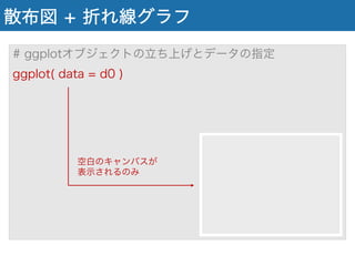
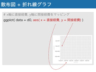
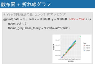
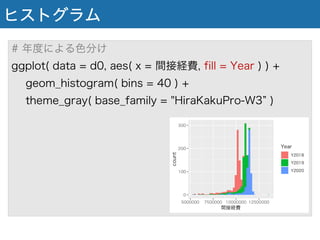
14. 散布図 + 折れ線グラフ
# Year列を各点の色（color）にマッピング
ggplot( data = d0, aes( x = 直接経費, y = 間接経費, color = Year ) ) +
geom_point( ) +
theme_gray( base_family = HiraKakuPro-W3 )

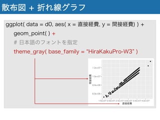
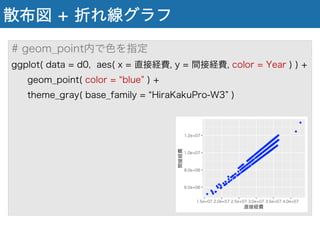
15. 散布図 + 折れ線グラフ
# geom_point内で色を指定
ggplot( data = d0, aes( x = 直接経費, y = 間接経費, color = Year ) ) +
geom_point( color = blue ) +
theme_gray( base_family = HiraKakuPro-W3 )

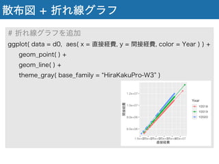
16. 散布図 + 折れ線グラフ
# 折れ線グラフを追加
ggplot( data = d0, aes( x = 直接経費, y = 間接経費, color = Year ) ) +
geom_point( ) +
geom_line( ) +
theme_gray( base_family = HiraKakuPro-W3 )

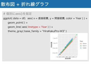
17. 散布図 + 折れ線グラフ
# 個別にaes()を指定
ggplot( data = d0, aes( x = 直接経費, y = 間接経費, color = Year ) ) +
geom_point( ) +
geom_line( aes( linetype = Year ) ) +
theme_gray( base_family = HiraKakuPro-W3 )

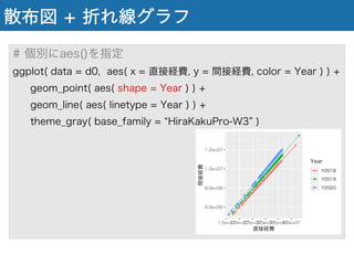
18. 散布図 + 折れ線グラフ
# 個別にaes()を指定
ggplot( data = d0, aes( x = 直接経費, y = 間接経費, color = Year ) ) +
geom_point( aes( shape = Year ) ) +
geom_line( aes( linetype = Year ) ) +
theme_gray( base_family = HiraKakuPro-W3 )

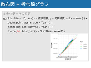
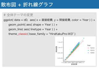
19. 散布図 + 折れ線グラフ
# 全体テーマの変更
ggplot( data = d0, aes( x = 直接経費, y = 間接経費, color = Year ) ) +
geom_point( aes( shape = Year ) ) +
geom_line( aes( linetype = Year ) ) +
theme_bw( base_family = HiraKakuPro-W3 )

20. 散布図 + 折れ線グラフ
# 全体テーマの変更
ggplot( data = d0, aes( x = 直接経費, y = 間接経費, color = Year ) ) +
geom_point( aes( shape = Year ) ) +
geom_line( aes( linetype = Year ) ) +
theme_classic( base_family = HiraKakuPro-W3 )

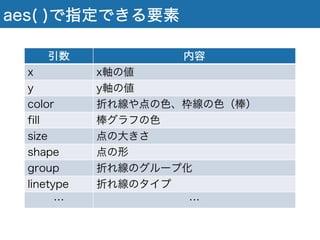
21. aes( )で指定できる要素
引数 内容
x x軸の値
y y軸の値
color 折れ線や点の色、枠線の色（棒）
fill 棒グラフの色
size 点の大きさ
shape 点の形
group 折れ線のグループ化
linetype 折れ線のタイプ
… …

22. ヒストグラム
# 最低限のヒストグラム
ggplot( data = d0, aes( x = 間接経費 ) ) +
geom_histogram( ) +
theme_gray( base_family = "HiraKakuPro-W3 )

23. ヒストグラム
# ビンの数を変更
ggplot( data = d0, aes( x = 間接経費 ) ) +
geom_histogram( bins = 40 ) +
theme_gray( base_family = "HiraKakuPro-W3 )

24. ヒストグラム
# 年度による色分け
ggplot( data = d0, aes( x = 間接経費, fill = Year ) ) +
geom_histogram( bins = 40 ) +
theme_gray( base_family = "HiraKakuPro-W3 )

25. ヒストグラム
# 棒の位置を変更
ggplot( data = d0, aes( x = 間接経費, fill = Year ) ) +
geom_histogram( bins = 40, position = identity ) +
theme_gray( base_family = "HiraKakuPro-W3 )

26. ヒストグラム
# 棒の色の透明度を変更
ggplot( data = d0, aes( x = 間接経費, fill = Year ) ) +
geom_histogram( bins = 40, position = identity , alpha = 0.5 ) +
theme_gray( base_family = "HiraKakuPro-W3 )

27. ヒストグラム
# 変数の値によってグラフを行に分割する
ggplot( data = d0, aes( x = 間接経費, fill = Year ) ) +
geom_histogram( bins = 40, position = identity ) +
theme_gray( base_family = "HiraKakuPro-W3 ) +
facet_grid( rows = vars( Year ) )

28. ヒストグラム
# 変数の値によってグラフを列に分割する
ggplot( data = d0, aes( x = 間接経費, fill = Year ) ) +
geom_histogram( bins = 40, position = identity ) +
theme_gray( base_family = "HiraKakuPro-W3 ) +
facet_grid( cols = vars( Year ) )

29. グラフの保存
# グラフを変数に保存する
g1 <- ggplot( data = d0, aes( x = 間接経費, fill = Year ) ) +
geom_histogram( bins = 40, position = identity ) +
theme_gray( base_family = "HiraKakuPro-W3 ) +
facet_grid( cols = vars( Year ) )
# グラフの書き出し
ggsave( output.png , g1 )
# サイズの変更（インチ）
ggsave( output2.png , g1, width = 9.6, height = 4.8 )